Numerical modelling of the thermospheric and ionospheric effects
of magnetospheric processes in the cusp region
A. A. Namgaladze1,2, A. N. Namgaladze1, M. A. Volkov1
1Polar Geophysical Institute, 15 Halturina St., Murmansk, 183010, Russia
2Murmansk State Technical University, 2 Sportivnaya St., Murmansk, 183010, Russia Received: 1 March 1996/Revised: 21 June 1996/Accepted: 25 June 1996
Abstract. The thermospheric and ionospheric effects of the precipitating electron flux and field-aligned-current variations in the cusp have been modelled by the use of a new version of the global numerical model of the Earth’s upper atmosphere developed for studies of polar phe-nomena. The responses of the electron concentration, ion, electron and neutral temperature, thermospheric wind velocity and electric-field potential to the variations of the precipitating 0.23-keV electron flux intensity and field-aligned current density in the cusp have been calculated by solving the corresponding continuity, momentum and heat balance equations. Features of the atmospheric grav-ity wave generation and propagation from the cusp region after the electron precipitation and field-aligned current-density increases have been found for the cases of the motionless and moving cusp region. The magnitudes of the disturbances are noticeably larger in the case of the moving region of the precipitation. The thermospheric disturbances are generated mainly by the thermospheric heating due to the soft electron precipitation and propa-gate to lower latitudes as large-scale atmospheric gravity waves with the mean horizontal velocity of about 690 m s~1. They reveal appreciable magnitudes at signifi-cant distances from the cusp region. The meridional-wind-velocity disturbance at 65°geomagnetic latitude is of the same order (100 m s~1) as the background wind due to the solar heating, but is oppositely directed. The ionospheric disturbances have appreciable magnitudes at the geomag-netic latitudes 70°—85°. The electron-concentration and -temperature disturbances are caused mainly by the ionization and heating processes due to the precipitation, whereas the ion-temperature disturbances are influence strongly by Joule heating of the ion gas due to the electric-field disturbances in the cusp. The latter strongly influence the zonal- and meridional-wind disturbances as well via the effects of ion drag in the cusp region. The results obtained are of interest because of the location of the
Correspondence to: A. A. Namgaladze
EISCAT Svalbard Radar in the cusp region and the asso-ciated observations at lower latitudes that will be possible using the existing EISCAT UHF and VHF radars. The paper makes predictions for both these regions, and these predictions will be tested by joint observations by ESR, EISCAT UHF/VHF and other ground-based iono-sphere/thermosphere observations.
1 Introduction
The cusp is a region where magnetosheath solar-wind particles have direct access to the magnetosphere and some of them may precipitate into the ionosphere. The local ionospheric effects of the soft electron precipitation in the cusp, such as increases in the F2-region electron concentration and temperature, are well known (Shep-herd, 1979). They have been modelled numerically, for example, by Roble and Rees (1977) by the use of the time-dependent, one-dimensional ionospheric model. The thermospheric effects of the soft electron precipitation are non-local, due to the internal atmospheric gravity waves propagating from the region of the abrupt electron pre-cipitation. The same can be said of the ionospheric and thermospheric effects of the field-aligned current vari-ations in the cusp because they influence the whole pattern of the polar ionosphere convection and related thermospheric disturbances. This means that these effects should be modelled by the use of the three-dimensional, time-dependent, self-consistent, ionospheric-thermo-spheric model including the electric-field calculations.
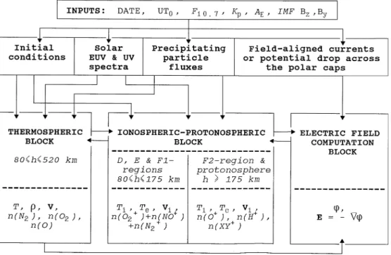
Fig. 1. Inputs, main computa-tion blocks and outputs of the model
study of the effect of a short-lived, localized enhancement in the high-latitude dawnside convection electric field has been made using the coupled ionospheric/thermosphere model (Millward et al., 1993). However, the magnetos-pheric convection electric-field variations were not cal-culated but taken as inputs in all these model simulations, and the cusp region was not considered as a separate high-latitude source of the thermospheric and ionospheric disturbances. This source has some specific features in comparison with other auroral sources being more local-ized in longitude and having lower characteristic energies of the precipitating electrons.
The main goal of this paper is to investigate the ther-mospheric and ionospheric effects of the soft electron precipitation and field-aligned current variations in the cusp, of the order of an hour in duration, using a new version of the global numerical model of the Earth’s upper atmosphere developed for studies of polar phenomena [Namgaladze et al., 1995 (1996a)]. This three-dimen-sional, time-dependent model describes the ionospheric, thermosphere and protonosphere of the Earth as a single system, and includes the calculations of the electric fields both of magnetospheric and thermospheric (dynamo) ori-gin. The questions wanted to be answered in our investi-gation are the following: How far from the cusp can the thermospheric and ionospheric effects of the precipitation be seen? How does the spatial distribution of the electric-field potential react to the variations of the electric-field-aligned currents in and near the cusp? How do these electric-field changes influence the disturbances of the thermospheric temperature and circulation and ionospheric parameters? What is the relative role of the electric-field penetration at remote distances from the cusp and atmospheric gravity wave propagation there?
The answers to these questions are of interest because of the location of the EISCAT Svalbard Radar in the cusp
region and the associated observations at lower latitudes that will be possible using the existing EISCAT UHF and VHF radars. This paper makes predictions for both these regions and these predictions will be tested by joint obser-vations by ESR, EISCAT UHF/VHF and other ground-based ionosphere/thermosphere observations.
2 The model
The global numerical model of the Earth’s upper atmo-sphere (Namgaladze et al., 1988, 1990, 1991, 1994) has been constructed at the Kaliningrad Observatory of IZ-MIRAN and modified for the polar ionosphere studies at the Polar Geophysical Institute in Murmansk [Nam-galadze et al., 1995 (1996a)]. The model describes the thermosphere, ionosphere and protonosphere of the Earth as a single system by means of numerical integration of the corresponding time-dependent, three-dimensional conti-nuity, momentum and heat balance equations for neutral, ion and electron gases, as well as the equation for the electric-field potential. It is the main difference of this global model from many others (e.g. Fuller-Rowell and Rees, 1980, 1983; Dickinson et al., 1981, 1984; Fuller-Rowellet al., 1984, 1987, 1988; Robleet al., 1988; Schunk, 1988; Sojka, 1989; Sojka and Schunk, 1988, 1989; Rich-mondet al., 1992; Roble and Ridley, 1994) that not only winds, gas densities and temperatures of the thermosphere and ionosphere, but electric fields both of thermospheric dynamo and magnetospheric origin and protonospheric parameters are calculated in this model as well.
electric-field computation blocks (see Fig. 1) using differ-ent coordinate systems and differdiffer-ent spatial grids of nu-merical integration. The exchange of information between these blocks is carried out at every time step of the numer-ical integration of the modelling equations.
In these blocks the corresponding well-known hydro-dynamical continuity, momentum and heat balance equa-tions for the neutral, electron and ion gases as well as the equation for the electric-field potential are all solved nu-merically by the use of the finite difference methods to obtain the time and spatial variations of the following parameters: the total mass densityo, concentrations of the main thermospheric gas constituentsn(O), n(O
2), n(N2), the total concentration of the molecular ions n(XY`)" n(O`2)#n(NO`)#n(N`2), concentrations of the atomic ions n(O`) and n(H`), temperatures of the neutral, ion and electron gases¹
n,¹iand¹e, thermospheric wind and ion velocity vectors V
n andVi, the electric-field potential u and the electric-field intensity vector E. The detailed
description of the model equations, initial and boundary conditions can be found in Namgaladzeet al. (1988).
In the thermospheric block the modelling equations are solved in a spherical geomagnetic coordinate system. The same coordinate system is used to calculate the concentra-tion, velocity and temperature of the molecular ions as well as the electron temperature at heights 80—175 km. The neutral-atmosphere parameters calculated in the spherical geomagnetic coordinate system are interpolated to the nodes of the finite difference magnetic dipole coor-dinate grid to calculate the parameters of the ionospheric F2 region and the protonosphere. In turn, the necessary parameters of the ion and electron gases are put into the thermospheric block from the ionospheric-protono-spheric block which uses the electric field from the elec-tric-field computation block. This latter block uses all necessary ionospheric and thermospheric parameters from the thermospheric and ionospheric-protonospheric blocks.
In our new version of this model [Namgaladzeet al., 1995 (1996a)] we use the variable latitudinal steps of numerical integration. For the thermospheric and mo-lecular ion parameters the latitudinal integration steps vary from 10° at the geomagnetic equator to 2° at the auroral zones; for the electric-field, ionospheric F2 region and protonospheric parameters they vary from 5°at the geomagnetic equator to 2°at the auroral zones. We have used this grid in the calculations presented below. Nam-galadzeet al. [1995 (1996a)] have shown that such a grid gives the results which do not differ significantly from those obtained with a regular grid using the constant 2°step in geomagnetic latitude. The time step of integra-tion is 2 min. Other steps of the numerical integraintegra-tion are 15° in geomagnetic longitude and variable in altitude: 3 km near the lower boundary (h"80 km), 5 km near h"115 km, 15 km near h"220 km, 25 km near h"330 km and 40 km nearh"500 km, giving 30 levels in the altitude range from 80 to 520 km for the thermo-spheric parameters. The number of the nodes of the grid along B for F2 region and protonospheric parameters
varies from 9 on the lowest equatorial field line to max-imum value 140 on the field line with¸"15.
3 The precipitating electron flux and field-aligned current variations
The input parameters of the model are 1) solar UV and EUV spectra; 2) precipitating particle fluxes; 3) field-aligned currents connecting the ionosphere with the magnetosphere. For the solar UV and EUV fluxes and their dependencies on solar activity we use the data from Ivanov-Kholodny and Nusinov (1987) for the low solar activity (F
10,7"70). Intensities of night-sky scattered radiation are put equal to 5 kR forj"121.6 nm and 5 R for each of other emission lines (jj"102.6, 58.4 and 30.4 nm). Spatial distribution of the precipitating electron fluxes is taken at the upper boundary of the thermosphere (h"520 km) in a simple form:
I(U,K)"I
mexp [!(U!Um)2/(DU)2!(K!Km)2/(DK)2], (1)
whereU and Kare geomagnetic latitude and longitude; K"0 corresponds to the midday geomagnetic meridian; I
mis the maximum intensity of the precipitating electron flux;U
m,Kmare the geomagnetic latitude and longitude of the precipitation maximum; DU,DK charcterize latitudi-nal and longitudilatitudi-nal dimensions of the precipitation area, respectively. All these parameters can vary depending on geophysical conditions.
We modelled the effects of the soft electron precipita-tion in the cusp by the following means. The precipitating 0.23-keV electron flux (a Maxwellian with characteristic energy of 0.23 keV) intensity in the cusp regionI
mand the geomagnetic latitude of the precipitation maximum U
m have been used as the variable inputs of the model; U
m varies between 78° and 73°geomagnetic latitude;DU" 3.5°; K
mcorresponds to the local midday;DK"45°, i.e. the cusp region extends approximately from 9 to 15 MLT. The undisturbed value of I
m has been chosen equal to 1.9]109cm~2s~1.
In the first variant of the calculations this flux was increased suddenly by a factor of 10 at 0000 UT and
Fig. 2a, b. Time variations of the precipitating 0.23-keV electron flux intensity (top) and geomagnetic latitude of the precipitation maximum (bottom) ina the fixed cusp position (left-hand plots) and
Fig. 4. Northern hemisphere geomagnetic polar plots (60°—90°) of the input field-aligned current density (left-hand plots) and calculated
electric-field potential (right-hand plots) at 0000 UT (top) and 0030 UT (bottom)
Fig. 3. Northern-hemisphere geomagnetic polar plot (60°—90°) of the input precipitation flux of 0.23-keV electrons in case of the moving cusp at 0030 UT
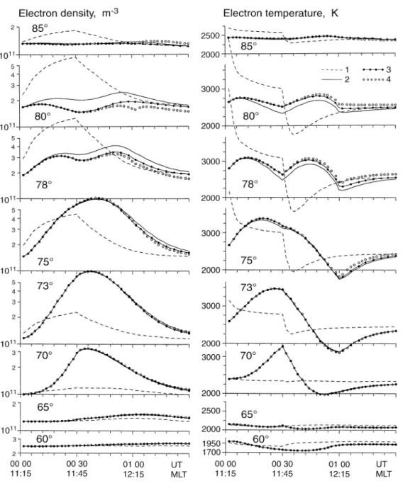
Fig. 5. Time variations of the calculated electron concentra-tion (left-hand plots) and elec-tron temperature (right-hand plots) ath"300 km,
K"240°, at various geomag-netic latitudes for variants 1 (dashed curves), 2 (solid curves), 3 (black-circle curves) and 4 (open circles) of the calculations (see text for ex-planation)
solar activity (for example, Namgaladze et al., 1996b) being close to those given by Hardy et al. (1985). They were not varied in these calculations.
The magnetospheric sources of the electric field for the undisturbed conditions are field-aligned currents in zones 1 and 2 (Iijima and Potemra, 1976). The first zone of field-aligned currents, flowing into the ionosphere on the dawn and out on the duskside, is at the polar-cap bound-ary ($76° magnetic latitude). The second zone of the field-aligned currents flowing opposite to the zone-1 cur-rents is located 4° equatorward from zone 1. The quiet field-aligned current density distribution in the north po-lar ionosphere at 0000 UT is shown here in Fig. 4 (left-hand, top panel).
To investigate the effects of the disturbed field-aligned current variations in the cusp for IMF B
y(0, we have used the following model input variations of the field-aligned currents based on the data by Taguchi et al.
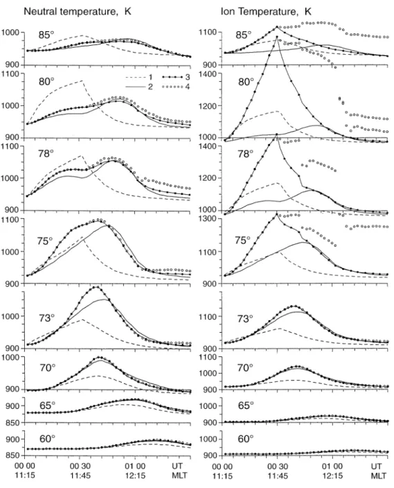
Fig. 6. The same as in Fig. 5 but for the neutral (left-hand plots) and ion (right-hand plots) temperature
cusp region is estimated approximately at 600 nT. Such a disturbance was observed in the cusp region when theB
y component of IMF was equal !9 nT (Taguchi et al., 1993). It means that the modelled situation corresponds to the case whenB
ychanges from 0 to!9 nT and back to 0 over a 1-h period.
4 The results of calculations and discussion
Four variants of the calculations have been performed: (1) the cusp position is fixed and only the sudden precipita-tion of 0.23-keV electrons takes place over 30 min (from 0000 to 0030 UT, see left-hand plots in Fig. 2); (2) the cusp is moving and the precipitation is linearly increased and then decreased over 1 h (see right-hand plots in Fig. 2); (3) the same as in variant 2 but the additional field-aligned
currents are included being linearly increased and then decreased over 1 h; (4) the same as in variant 3 but the additional field-aligned currents maintain their maximum values after 0030 UT.
The magnetosphere may generate these four cases by the following means. Variant 1 employs a square wave pulse of enhanced electron precipitation flux in the cusp region, which maintains a fixed position in the ionosphere. This could well be the result of a corresponding pulse in the density of the solar wind impinging on the magneto-sphere. Such a pulse would compress the dayside mag-netosphere but would not move the latitude of the dayside cusp in the ionosphere (because the ionosphere is largely incompressible, in the sense that the magnetic field there is almost constant).
Fig. 7. The same as in Fig. 5 but for the meridional, positive northward (left-hand plots) and zonal, positive eastward (right
-hand plots) thermospheric wind velocity
solar-wind density. The cusp migrates equatorwards, as is often seen in observations. This would be expected if the magnetopause compression were to be accompanied by a proportionally enhanced rate of magnetopause recon-nection, eroding the dayside magnetopause and bringing the cusp to lower latitudes. However, we would also expect (after about a 10—15-min delay) this to cause a rise in the field-aligned currents and associated ionospheric con-vection (see for example Cowley and Lockwood, 1992). Thus variant 2 is unlikely to be observed. Nevertheless, it is useful to model variant 2, as it helps distinguish the effects of the precipitation from those of the elec-trodynamics. We consider variant 3, in which the erosion is accompanied by field-aligned currents in synchroniza-tion with erosion, to be more realistic than variant 2.
Lastly, variant 4 does not ramp down the field-aligned currents after the rise; this means that the cusp-region currents and associated flows persist after the enhanced
cusp precipitation decays. This would happen if the day-side reconnection persists after the decay of the solar-wind pressure pulse. This situation would thus apply to a south-ward turning of the IMF, occuring at the time of the solar-wind pressure pulse.
Figures 5—7 show the calculated time variations of the ionospheric and thermospheric parameters at various north geomagnetic latitudes in the range 60°—85°for the daytime 240°geomagnetic meridian at the height 300 km. Variants 1, 2, 3 and 4 of the calculations are presented in these figures by the dashed, solid, black-circle and open-circle curves, respectively.
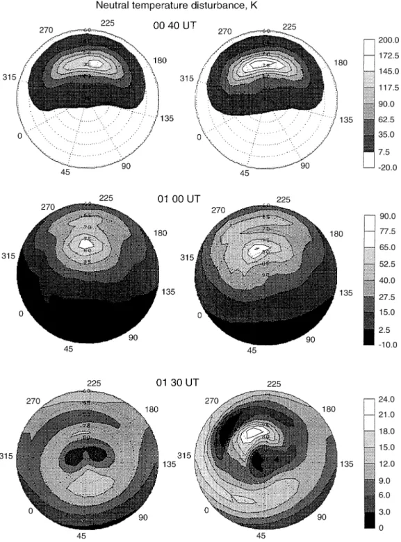
Fig. 8. North geomagnetic polar plots (60°—90°) of the calculated neutral-temper-ature disturbance at
h"300 km in variants 2 (left-hand plots) and 3 (right-hand plots) of the calculations at 0040, 0100 and 0130 UT
minimal in case of the fixed cusp position (variant 1 of the calculations). The exception for this is the initial electron temperature burst near the cusp region in the beginning of the abrupt precipitation. This burst takes place when the ion concentration is not yet high enough to cool the electron gas effectively.
At the end of the precipitation burst (0030 UT) in variant 1, electron concentrationN
e at h"300 km (left-hand plots in Fig. 5) reaches its maximum value of about 8.4]1011m~3at 78°geomagnetic latitude, in comparison
with the initial value of about 2.9]1011m~3at 0000 UT. This then decreases to the quiet level during the next 30 min. In the case of the moving cusp (variant 2 of the calculations)N
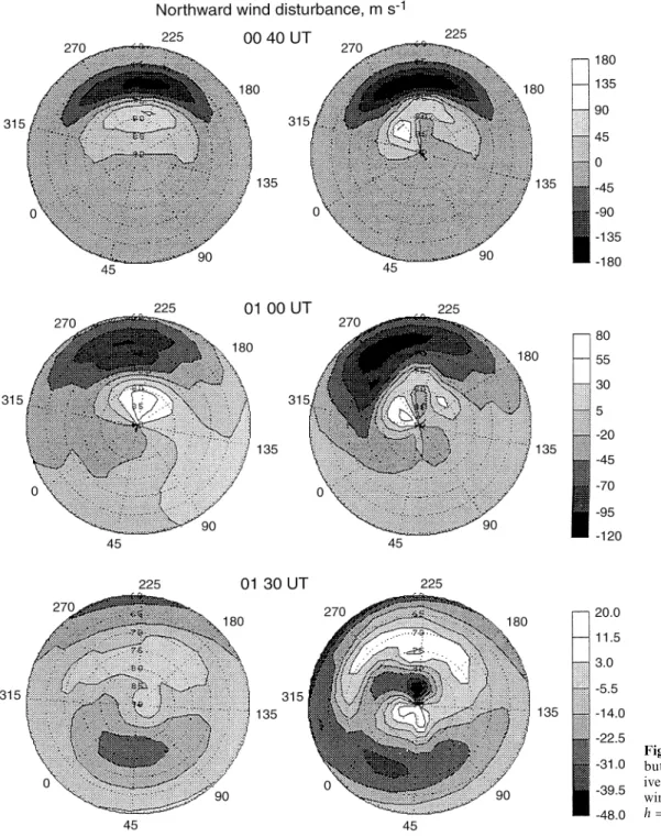
Fig. 9. The same as in Fig. 8 but for the meridional (posit-ive northward) thermospheric-wind-velocity disturbance at
h"300 km ion-temperature disturbances. At 70° geomagnetic
lati-tude, theN
eenhancement is still rather high in variant 2 of the calculations, whereas in variant 1 the disturbance magnitude drops very significantly. At lower latitudes, only weak positive disturbances ofN
ecaused by the dis-turbed-thermospheric-wind action propagate equator-wards with average speed of about 540 m s~1 in both variants of the calculations as estimated for the 65°—60° latitude range.
The electron-temperature disturbances are shown in Fig. 5 (right-hand plots). They are positive in the cusp region for most of the time when the heating of the electron gas by the precipitating electrons is active, but
become negative after the ending of the precipitation. This is because the remaining increased ion concentration acts to cool the electron gas.
Fig. 10. The same as in Fig. 8 but for the zonal (positive eastward) thermospheric-wind-velocity disturbance at
h"300 km The meridional thermospheric wind disturbances
(left-hand plots in Fig. 7), driven by the pressure gradient forcing from the heated cusp region, reveal an analogous character of the propagation being of about 140, 90 and 46 m s~1in magnitude at the geomagnetic latitudes 70°, 65°and 60°, respectively, in case of the moving cusp. The corresponding values are about 90, 50 and 26 m s~1 at the same latitudes in case of the fixed cusp position. The zonal-wind disturbances (right-hand plots in Fig. 7) are insignificant in the midday sector for cases when only enhanced precipitation takes place. The neutral-composi-tion disturbances (not shown) are virtually confined to the cusp region where the concentration O/N
2 ratio dimin-ishes by about 25% at 75°geomagnetic latitude in case of
the moving cusp, and 24% at 80°in case of the fixed cusp position.
Now let us consider the results of the calculations in variants 3 and 4 where the additional field-aligned cur-rents in the cusp region are included as shown in Fig. 4. These have largest current densities at 0030 UT and sub-sequently either return to the quiet at 0100 UT (variant 3) or remain fixed at their maximum values (variant 4).
to empirical models (for example that by Heppner and Maynard, 1987). The disturbed potential pattern (bottom panel) obtained when the additional field-aligned currents are included, consists of three convection cells: two with positive potential values in the midday-morning sector and one with negative potential in the evening sector. Such a convection pattern corresponds to the type G dis-cussed by Reiff and Burch (1985). The maximum electric-field intensities are of about 30 mV m~1.
Figures 8—10 show the geomagnetic polar plots (60°—90°) of the calculated thermospheric disturbances, i.e. the differences between disturbed and undisturbed values of the calculated neutral temperature, meridional (positive northward) and zonal (positive eastward) wind velocity at 300-km altitude. A comparison of the results shown in the left- and right-hand columns in these figures, as well as of the results presented by solid curves with and without the black circles in Figs. 5—7, demonstrates the differences between the effects caused by the joint action of the precipitation and field-aligned-current variations, and those caused by the precipitation only. It can be seen from these figures that the main differences are in the thermo-spheric-wind and ion-temperature disturbances in the cusp region. The latter are much more intensive (up to about 600 K) at the geomagnetic latitudes 75°—80°in the case of joint precipitation and field-aligned-current action due to Joule heating of the ion gas in the cusp region, whereas the neutral-temperature increases are not so great (Figs. 6 and 8).
The most significant changes are in the variations in zonal thermospheric wind due to the ion drag. Eastward wind disturbances of about 140—200 m s~1 appear at geomagnetic latitudes 75°—80° in the midday sector (Fig. 7) and of about 200—300 m s~1in the afternoon sec-tor (Fig. 10). The meridional wind disturbances are about 90 m s~1at the geomagnetic latitudes 80°—85°in the mid-day sector (Fig. 7) and of about 180 m s~1 in the after-noon sector (Fig. 9). They are also caused by the ion drag which acts in the opposite direction, in comparison with the pressure gradient forcing in the midday sector.
The response of electron density to the field-aligned-current disturbances (Fig. 5) is very localized near the 80° geomagnetic latitude, being negative because of an in-crease in ion temperature due to Joule heating of the ion gas. The electron-temperature change is insignificant. The differences between the results of the calculations in vari-ants 3 and 4 are seen in Figs. 6 and 7 to be largely in the ion-temperature and the zonal- and meridional-thermo-spheric-wind variations at the geomagnetic latitudes 75°—85°.
5 Summary and conclusions
The thermospheric and ionospheric effects of the precipi-tating electron flux and field-aligned-current variations in the cusp have been modelled by the use of a global numerical model of the Earth’s upper atmosphere. This three-dimensional, time-dependent model describes the ionosphere, thermosphere and protonosphere of the Earth as a single system and includes the calculations of the
electric fields, both of magnetospheric and thermospheric (dynamo) origin. A new version of this model, developed for studies of polar phenomena, employs variable latitudi-nal steps in the numerical integration scheme of the coupled equations, allowing us to enhance the latitudinal resolution of the model at those latitudes where this is necessary.
The responses of the electron concentration, ion, elec-tron and neutral temperature, wind velocity and electric-field potential to the variations of a precipitating 0.23-keV electron flux intensity with and without variations in the field-aligned current density in the cusp have been cal-culated by solving the corresponding continuity, mo-mentum and heat-balance equations.
Four variants of the calculations have been performed: (1) the cusp position is fixed and only the sudden precipi-tation of 0.23-keV electrons takes place over 30 min; (2) the cusp is moving from 78°to 73°and back and the precipitation flux is linearly increased and then decreased over 1 h; (3) the same as in variant 2 but additional field-aligned currents corresponding to IMF B
y(0 are included, being linearly increased and then decreased over 1 h; (4) the same as in variant 3 but the additional field-aligned currents maintain their maximum values after 0030 UT.
The main prominent feature of the results of our calcu-lations is that the thermospheric disturbances outside the cusp are generated mainly by the thermospheric heating due to the soft electron precipitation. They reveal appreci-able magnitudes at significant distances from the cusp region being noticeably larger in case of the moving region of the precipitation. For example, the meridional-wind-velocity disturbance at 65°geomagnetic latitude is of the same order as the background wind due to solar heating, but is oppositely directed. We can conclude from these calculations that the most distinguishable disturbances outside the cusp are those of the thermospheric wind. It means that Fabri-Perot interferometer observations out-side the cusp could be used as a means of remote invest-igation of the cusp dynamics.
The thermospheric disturbances propagate from the cusp to lower latitudes as large-scale atmospheric gravity waves with the mean horizontal velocity of about 690 m s~1. This speed is comparable with values of about 400—718 m s~1, estimated from the observations of AGW (with periods of about 60 min) during the October 1985 WAGS campaign (Riceet al., 1988; Williamset al., 1988). It is worth nothing that at the geomagnetic latitudes equatorwards from 70°, all disturbances have a similar form of time variation, almost independent of the time variation of the cusp disturbance. This arises because of the attenuation of the higher-frequency harmonics.
disturbances via ion drag, so these disturbances can reach values of about 200—300 m s~1in the afternoon sector at 75°—85°geomagnetic latitude.
Acknowledgements. This work is supported by Grants RLX300 from the International Science Foundations and Russian Govern-ment and 95-05-14505 from the Russian Foundation of Funda-mental Investigations, and by the Grant from the SCOSTEP Bureau (1995). The authors would like to thank O. V. Martynenko for his assistance in performing the calculations. We are grateful to the refereed1 for very useful remarks and comments.
Topical Editor D. Alcayde´ thanks M. Lockwood and A. G. Burns for their help in evaluating this paper.
References
Burns, A. G., T. L. Killeen, and R. G. Roble,A theoretical study of thermospheric composition perturbations during an impulsive geomagnetic storm,J.Geophys.Res.,96,14153, 1991.
Cowley, S. W. H., and M. Lockwood,Excitation and decay of solar wind driven flows in the magnetosphere-ionosphere system,Ann.
Geophysicae,10,103, 1992.
Dickinson, R. E., E. C. Ridley, and R. G. Roble,A three-dimensional general circulation model of the thermosphere,J.Geophys.Res.,
86,1499, 1981.
Dickinson, R. E., E. C. Ridley, and R. G. Roble,Thermospheric general circulation with coupled dynamics and compositions,J.
Atmos.Sci.,41,205, 1984.
Fuller-Rowell, T. J.,A two-dimensional, high-resolution, nested-grid model of the thermosphere 1. Neutral response to an electric field ‘‘spike’’,J.Geophys.Res.,89,2971, 1984.
Fuller-Rowell, T. J., and D. Rees,A three-dimensional, time-depen-dent global model of the thermosphere,J.Atmos.Sci.,37,2545, 1980.
Fuller-Rowell, T. J., and D. Rees,A three-dimensional, time-depen-dent simulation of the global dynamical response of the thermo-sphere to a geomagnetic substrom,J.Atmos.¹err.Phys.,43,701, 1981.
Fuller-Rowell, T. J., and D. Rees, Derivation of a conservation equation for mean molecular weight for a two-component gas within a three-dimensional, time-dependent model of the ther-mosphere,Planet.Space Sci.,31,1209, 1983.
Fuller-Rowell, T. J., and D. Rees,Interpretation of anticipated long-lived vortex in the lower thermosphere following simulation of an isolated substorm,Planet.Space Sci.,32,69, 1984.
Fuller-Rowell, T. J., D. Rees, S. Quegan, G. J. Bailey, and R. J. Moffett,The effect of realistic conductivities on the high-latitude neutral thermospheric circulation, Planet.Space Sci., 32, 469, 1984.
Fuller-Rowell, T. J., D. Rees, S. Quegan, G. J. Bailey, and R. J. Moffett, Interactions between neutral thermospheric composi-tion and the polar ionosphere using a coupled ionosphere-ther-mosphere model,J.Geophys.Res.,92,7744, 1987.
Fuller-Rowell, T. J., D. Rees, S. Quegan, R. J. Moffett, and G. J. Bailey,Simulations of the seasonal and universal time variations of the high-latitude thermosphere and ionosphere using a coupled, three-dimensional model,Pure Appl.Geophys.,127,
189, 1988.
Fuller-Rowell, T. J., D. Rees, H. Rishbeth, A. G. Burns, T. L. Killeen, and R. G. Roble, Modelling of composition changes during F-region storms: a reassessment.J.Atmos.¹err.Phys.,53,541, 1991.
Hardy, D. A., M. S. Gussenhoven, and E. Holeman,A statistical model of auroral electron precipitation, J. Geophys. Res., 90,
4229, 1985.
Heppner, J. P., and N. C. Maynard,Empirical high-latitude electric field models,J.Geophys.Res.,92,4467, 1987.
Iijima, T., and T. A. Potemra,The amplitude distribution of field-aligned currents at northern high latitudes observed by Triad.
J.Geophys.Res.,81,2165, 1976.
Ivanov-Kholodny, G. S., and A. A. Nusinov,Korotkovolnovoe iz-luchenie Solntza i ego vozdeistvie na verchnyuu atmospheru i ionospheru, Issled.cosmicheskogo prostransiva (Invest.Outer Space),»INI¹I Press,Moscow,26,80, 1987.
Maeda, S., T. J. Fuller-Rowell, and D. S. Evans,Zonally averaged dynamical and compositional response of the thermosphere to auroral activity during September 18—24, 1984,J.Geophys.Res.,
94,16869, 1989.
Millward, G. H., S. Quegan, R. J. Moffett, T. J. Fuller-Rowell, and D. Rees, A modelling study of the coupled ionospheric and thermospheric response to an enhanced high-latitude electric field events,Planet.Space Sci.,41,45, 1993.
Namgaladze, A. A., Yu. N. Korenkov, V. V. Klimenko, I. V. Karpov, F. S. Bessarab, V. A. Surotkin, T. A. Glushchenko, and N. M. Naumova,Global model of the thermosphere-iono-sphere-protonosphere system,Pure Appl.Geophys. A. A.,127,
219, 1988.
Namgaladze, A. A., Yu. N. Korenkov, V. V. Klimenko, I. V. Karpov, F. S. Bessarab, V. A. Surotkin, T. A. Glushchenko, and N. M. Naumova,Global numerical model of the thermosphere, iono-sphere, and protonosphere of the Earth,Geomagn.Aeron.,30,
612, 1990.
Namgaladze, A. A., Yu. N. Korenkov, V. V. Klimenko, I. V. Karpov, V. A. Surotkin, and N. M. Naumova,Numerical modelling of the thermosphere-ionosphere-protonosphere system,J.Atmos.¹err.
Phys.,53,1113, 1991.
Namgaladze, A. A., Yu. N. Korenkov, V. V. Klimenko, I. V. Karpov, V. A. Surotkin, F. S. Bessarab, and V. M. Smertin,Numerical modelling of the global coupling processes in the near-earth space environment,COSPAR Coll.Ser.,5,807, 1994.
Namgaladze, A. A., O. V. Martynenko, and A. N. Namgaladze,
Global model of the upper atmosphere with variable latitudinal steps of numerical integration,IºGG XXI General Assembly,
Boulder,1995, Abstracts,GAB41F-6, B150, 1995 (and in Russian
Geomagn.Aeron.,36,89, 1996a).
Namgaladze, A. A., O. V. Martynenko, A. N. Namgaladze, M. A. Volkov, Yu. N. Korenkov, V. V. Klimenko, I. V. Karpov, and F. S. Bessarab,Numerical simulation of an ionospheric disturbance over EISCAT using a global ionospheric model,J.Atmos.¹err.
Phys.,58,297, 1996b.
Ohtani, S., T. A. Potemra, P. T. Newell, L. J. Zanetti, T. Iijima, M. Watanabe, L. G. Blomberg, R. D. Elphinstone, J. S. Murphree, M. Yamauchi, and J. G. Woch,Four large-scale field-aligned current systems in the dayside high-latitude region,J.Geophys.
Res.,100,137, 1995.
Reiff, P. H., and J. L. Burch,IMF-B
y-dependent plasma flow and
Birkeland currents in the dayside magnetosphere. 2. A global model for northward and southward IMF,J.Geophys.Res.,90,
1595, 1985.
Rice, D. D., R. D. Hunsucker, L. J. Lanzerotti, G. Growley, P. J. S. Williams, J. D. Graven, and L. Frank,An observation of atmo-spheric gravity wave cause and effect during the October 1985 WAGS campaign,Radio Sci.,23,919, 1988.
Richmond, A. D., and S. Matsushita, Thermospheric response to a magnetic substorm,J.Geophys.Res.,80,2839, 1975.
Richmond, A. D., E. C. Ridley, and R. G. Roble,A thermosphere-ionosphere general circulation model with coupled electro-dynamics,Geophys.Res.¸ett.,19,601, 1992.
Roble, R. G., M. H. Rees,Time-dependent studies of the aurora: effects of particle precipitation on the dynamic morphology of ionospheric and atmospheric properties,Planet.Space Sci.,25,
991, 1977.
Roble, R. G., and E. C. Ridley,A thermosphere-ionosphere-meso-sphere-electrodynamics general circulation model (TIME-GCM): equinox solar cycle minimum conditions (30—500 km),
Geophys.Res.¸ett.,21,417, 1994.
Roble, R. G., J. M. Forbes, and F. A. Marcos, Thermospheric dynamics during the March 22, 1979, magnetic storm., 1. Model simulations.J.Geophys.Res.,92,6045, 1987.
Roble, R. G., E. C. Ridley, A. D. Richmond, and R. E. Dickinson, A coupled thermosphere/ionosphere general circulation model,
Sandholt, P. E., C. J. Farrugia, L. F. Burlaga, J. A. Holte´t, J. Moen, B. Lybekk, B. Jacobsen, D. Opsvik, A. Egeland, R. Lepping, A. J. Lazarus, T. Hansen, A. Brekke, and E. Friis-Christensen,
Cusp/cleft auroral activity in relation to solar wind dynamic pressure, interplanetary magnetic field B
z and By,J.Geophys. Res.,99,17323, 1994.
Schunk, R. W., A mathematical model of the middle and high-latitude ionosphere,Pure Appl.Geophys.,127,255, 1988.
Shepherd, G. S.,Dayside cleft aurora and its ionospheric effects,Rev.
Geophys.Space Phys.,17,2017, 1979.
Sojka, J. J.,Global-scale physical models of the F-region iono-sphere,Rev.Geophys.,27,371, 1989.
Sojka, J. J., and R. W. Schunk,A model study of how electric field structures affect the polar cap F-region,J.Geophys.Res.,93,884, 1988.
Sojka, J. J., and R. W. Schunk,Theoretical study of the seasonal behavior of the global ionosphere at solar maximum,J.Geophys.
Res.,94,6739, 1989.
Taguchi, S., M. Sugiura, J. D. Winningham, and J. A. Slavin, Charac-terization of the IMF-B
y-dependent field-aligned currents in the
cleft region based on DE 2 observations,J.Geophys.Res.,98,
1393, 1993.
Williams, P. J. S., G. Growley, K. Schlegel, T. S. Virdi, I. McCrea, G. Watkins, N. Wade, J. K. Hargreaves, T. Lachlan-Cope, H. Muller, J. E. Baldwin, P. Warner, A. P. van Eyken, M. A. Hapgood, and A. S. Rodger,The generation and propagation of atmospheric gravity waves observed during the Worldwide At-mospheric Gravity-wave study (WAGS),J.Atmos.¹err.Phys.,
50,323, 1988.
Yamauchi, M., R. Lundin, and J. Woch,The interplanetary magnetic field B
y effects on large-scale field-aligned currents near local
noon: contributions from cusp part and non-cusp part,J.Geo