Assessing the impact of closely-spaced intersections on traffic operations and pollutant emissions on a corridor level

Assessing the impact of closely-spaced intersections on traffic operations

and pollutant emissions on a corridor level

Fernandes P. a*, Coelho, M.C. a, Rouphail, N.M b

a Department Mechanical Engineering / Centre for Mechanical Technology and Automation (TEMA), University of Aveiro, Campus Universitário de Santiago, 3810-193 Aveiro - Portugal

b Institute for Transportation Research and Education/ North Carolina State University, North Carolina State University, Campus Box 8601, Raleigh, NC 27695-8601

* PhD Student, Mechanical Engineering, E-mail: paulo.fernandes@ua.pt

University of Aveiro, Dept. Mechanical Engineering / Centre for Mechanical Technology and Automation (TEMA), University of Aveiro, Campus Universitário de Santiago, 3810-193 Aveiro - Portugal

ABSTRACT

Traffic lights or roundabouts along corridors are usually installed to address location-specific operational needs. An understanding of the impacts on traffic regarding to highly-congested closely-spaced intersections has not been fully addressed. Accordingly, consideration should be given to how these specific segments affect corridor performance as a whole.

One mixed roundabout/traffic light/stop-controlled junctions corridor was evaluated with the microscopic traffic model (VISSIM) and emissions methodology (Vehicle Specific Power – VSP). The analysis was focused on two major intersections of the corridor, a roundabout and a traffic light spaced lower than 170 meters apart under different traffic demand levels. The traffic data and corridor geometry were coded into VISSIM and compared with an alternative scenario where the traffic light was replaced by a single-lane roundabout. This research also tested a method to improve corridor performance and emissions by examining the integrated effect of the spacing between these intersections on traffic delay and vehicular emissions (carbon dioxide, monoxide carbon, nitrogen oxides, and hydrocarbons). The Fast Non-Dominated Sorting Genetic Algorithm (NSGA-II) was used to find the optimal spacing for these intersections.

The analysis showed that the roundabout could achieve lower queue length (~64%) and emissions (16-27%, depending on the pollutant) than the traffic light. The results also suggested that 200 meters of spacing using the best traffic control would provide a moderate advantage in traffic operations and emissions as compared with the existing spacing. Keywords: Intersections, Multi-objective optimization, Micro-scale modeling, Spacing.

ABRREVIATION INDEX

a Vehicle instantaneous acceleration or deceleration [m.s-2_] AADT Average Annual Daily Traffic

CO Carbon Monoxide

CO2 Carbon Dioxide

DPV Diesel Passenger Vehicles

DTA Dynamic Traffic Assignment

EU European Union

FHWA Federal Highway Administration

GA Genetic Algorithm

GEH Geoffrey E. Havers Statistic

GPS Global Positioning System

GPV Gasoline Passenger Vehicles

grade Terrain gradient [decimal fraction]

HC Hydrocarbons

HCM Highway Capacity Manual

HDV Heavy-Duty Vehicles

K-S Two-sample Kolmogorov-Smirnov test

LDDT Light Duty Diesel Trucks

LOS Level of Service

LPV Light Passenger Vehicles MAPE Mean Absolute Percent Error

NCHRP National Cooperative Highway Research Program

NOX Nitrogen Oxides

OBD On-Board Diagnostic System

O-D Origin-Destination matrices

POF Pareto Approximate Front

S Spacing between intersections [m]

US United States

v Vehicle instantaneous speed [m.s-1_] VISSIM Verkehr In Städten SIMulationsmodell VSP Vehicle Specific Power [kW.ton-1_]

1. INTRODUCTION AND RESEARCH OBJECTIVES

Urban sprawl is known worldwide as the uncontrolled expansion of low-density and single-use suburban development. More than 25% of the European Union’s (EU) territory has been directly affected by urban land use (EEA, 2006), and nearly 75% of Europeans live in urbanized areas (UN, 2014). The impact from urban ways of living has increasingly more repercussions well beyond city boundaries. Thus, cities are the defining ecological phenomenon of the 21st century as they have become the major engine of economic development (Newman and Jennings, 2012). Concurrently the phenomenon of urbanization is continuously eroding the countryside and making the boundary between cities and their suburban areas virtually undistinguishable.

A representative example of the above issues is found within urban arterials. Series of intersections along corridors are usually implemented according to the available space and do not follow any specific design criteria (Association et al., 2012). Some of these traffic facilities are located in close proximity to each other (due to constraints in terms of land use), and the queue spillback from a downstream intersection can adversely affect the upstream throughput, and, as a result, the overall corridor performance.

Although research of the impacts on traffic performance and emissions of different traffic controls at isolated intersections and an arterial level has been conducted, little attention has been given to the real impacts on traffic regarding the short spacing between adjacent intersections. There is a concern that under specific traffic demands and intersection control (e.g. traffic light or roundabout) the impacts of specific segments of the corridor may be different by varying the spacing between intersections. In addition, the optimization of a particular pollutant (carbon dioxide – CO2, carbon monoxide – CO, nitrogen oxides – NOX and hydrocarbons – HC) could dictate different optimal spacing.

The main contributions of this study to the current state-of-art are the following: 1) Understanding the impact of highly-congested closely-spaced intersections within corridors; 2) Implementing a multi-criteria analysis to assess the optimal spacing between intersections to improve corridor-specific operations; and 3) Including specific pollutant criteria (global pollutants which have impacts on global warming; local pollutants which affect human health) to account corridor-specific environmental concerns.

One mixed roundabout/traffic light/stop-controlled junctions corridor is evaluated with the microscopic traffic model (VISSIM) and emissions methodology (Vehicle Specific Power – VSP). After that, a multi-objective genetic algorithm is used to search intersections-optimal spacing and the results are compared with existing conditions. Thus, the objective of this paper is twofold:

1. To compare the impacts of different closely-spaced traffic controls within a corridor on vehicle delay, and global (CO2) and local (CO, NOX and HC) pollutant emissions; 2. To find the optimal spacing values for the intersections considering the best traffic

control.

The second section offers a review of the technical literature on this topic. The methodology used in this paper is explained in the third section. Analysis results and policy implications

are presented and discussed in the fourth section, followed by the main conclusions of this study in the fifth section.

2. LITERATURE REVIEW

Spacing between intersections, both in terms of frequency and uniformity, governs the performance of urban and suburban roadways. Hence, the establishment of intersection spacing criteria for an arterial is one of the most important and basic access management techniques (Gluck et al., 1999). There is no universally formal rule for the minimum spacing between adjacent intersections (SETRA, 2002). As with standards for driveway spacing, the optimal spacing between signalized intersections depends on the speed, the traffic demand, and the intersection layout (Fwa, 2005).

In North America and Europe, various design manuals propose threshold spacing values for signalized and unsignalized intersections. The National Cooperative Highway Research Program (NCHRP) Report 420 provides a range of optimum signal spacing values as a function of speed and cycle length for non-coordinated signals (Gluck et al., 1999). For instance, intersections spaced at about 330 meters from each other can provide progressive speeds up to 50 km/h at cycle lengths from 60 to 70 seconds. For cycle lengths higher than 100 seconds only spacing values above 600 meters guarantee progressive speeds of 50 km/h. Gluck et al. (1999) suggest that each additional signal over two per mile (400 meters of spacing) increases travel time by 7%. The Transportation Research Board Access Management Manual recommends that spacing between major urban arterials should be equal or higher than 800 meters considering an Average Annual Daily Traffic (AADT) between 2,000 and 15,000 vehicles (TRB, 2003). Whereas, French guidelines state that a minimum spacing of 250 meters can be adopted whether site characteristics have conditions to make this feasible (SETRA, 2002).

The Colorado Access Demonstration Project found that 800 meters of spacing can reduce vehicle-hours of delay and travel by 60% and 50%, respectively, compared with signals spaced at 400 meters with full median openings (TRB, 2003). According to the arterial segment running time formula in Highway Capacity Manual (HCM), time spent at arterials increases as average spacing increases. However, HCM method does not take account for the effect of queue spillback from a downstream signal (HCM, 2010).

Synchronization of adjacent traffic lights (green waves) helps to reduce vehicle stops and delay. The Federal Highway Administration (FHWA) suggests that spacing shorter than 300 meters is difficult to coordinate on arterials which have the same signal controller (FHWA, 2013). Tarko et al. (2008) explain that good coordination for conventional signalized intersections with protected turn bays is only attained for equally spaced intersections in both directions of traveling.

The current research on emissions and fuel consumption at different corridors with traffic lights (Barth and Boriboonsomsin, 2012; Guo and Zhang, 2014; Kwak et al., 2012; Park et al., 2009; Xia et al., 2012) and mixed traffic lights/roundabouts corridors (Coelho et al., 2009a; Hallmark et al., 2010; Hallmark et al., 2011; Nicoli et al., 2015) is extensive, but does not explore the influence of spacing on traffic operations.

Recently, urban roundabout corridors have become more prevalent in the United States (US) and Europe. As such, several studies have been performed to assess roundabout corridors

performance in terms of capacity and emissions (Bugg et al., 2015; Fernandes et al., 2015a; Fernandes et al., 2015b; Isebrands et al., 2008; Krogscheepers and Watters, 2014). In particular, Fernandes et al. (2015b) demonstrated that spacing between roundabouts had an impact on the spatial distribution of CO2 emissions (R-squared >0.50), especially in the case of closely-spaced roundabouts (<170 meters). However, the above-mentioned research did not include an in-depth assessment of the spacing on traffic operations. Concurrently, additional relevant research on environmental impacts in conventional (Chevallier et al., 2009; Coelho et al., 2006; Mudgal et al., 2014; Várhelyi, 2002) and innovative (Guerrieri et al., 2015; Tollazzi et al., 2015) roundabouts did not address the impacts of nearby upstream/downstream intersections.

One of the main conclusions gained from the literature review is the realization that there is a higher need for systematic analysis on the impact that specific segments of a corridor with high traffic flows have on overall corridor performance. Furthermore, little is known about the effect that spacing could have on traffic performance and emissions. Lastly, a proper selection to gain optimal spacing between intersections to improve simultaneously traffic performance and emissions should also be explored.

The novel purpose of this research is to evaluate a specific segment of a corridor to provide some evidences about what the causes of its impacts might be. After that, several methods to improve the performance and emissions of the overall corridor are investigated, namely: 1) replacement of the existing traffic control; and 2) placement of such intersection (within feasible distances) along the mid-block section. Finally, this research tests and verifies these methods in a real word urban corridor. The effects of spacing distances were hypothesized to be different for each pollutant and concomitantly lead to a trade-off analysis among the selected variables, namely:

1. Low spacing between intersections along an arterial will have a negative impact on CO2 emissions and traffic performance and at the same time can have a different effect on local pollutants, since vehicles have a very short distance to reach high speeds (overlapping of the intersections influence areas);

2. High spacing could reduce delay and CO2 emissions, but may be diverse in local pollutants, because vehicles attain high speeds at mid-block area, and they could experience high acceleration/deceleration rates at the downstream and upstream areas of either intersections.

3. METHODOLOGY

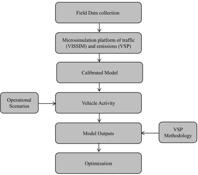
The core idea of the proposed methodology was to introduce a microsimulation framework to assess traffic performance and emissions of an existing corridor as well as to implement future operational scenarios. The methodology is explained in five steps. First, data were collected in the selected baseline site. Second, the network was coded, latter calibrated, and validated for the baseline site using the microsimulation platform of traffic and emissions. Third, different operational scenarios were defined and compared. Fourth, emissions were estimated using VSP. Step five was focused on the optimization of the results using a multi-objective analysis. The modeling framework is exhibited in Figure 1.

3.1. Microsimulation platform of traffic and emissions 3.1.1. Traffic Modeling

VISSIM (German acronym for Verkehr In Städten SIMulationsmodell) microsimulation model is recognized as a powerful tool for corridors with different forms of intersections in order to perform reliable operational assessment, namely: a) to define different parameters of driving behavior for roundabouts and traffic lights as car-following models or gap-acceptance (PTV, 2011); b) to simulate fixed-cycle signal controls (PTV, 2011); c) to calibrate and validate a wide range of parameters to set faithful representations of the traffic on an arterial level for capacity and emissions’ purposes, as demonstrated elsewhere (Bared and Edara, 2005; Fernandes et al., 2015a; Hallmark et al., 2010); and d) to enable storing and exporting vehicle dynamics data at high time resolutions that can be used by external emissions models.

3.1.2. Emission Modeling

Vehicular emissions were estimated using VSP methodology (USEPA, 2002) for four main reasons: 1) it allows estimating instantaneous emissions based on second-by-second vehicle activity data, taking the trajectory files given by VISSIM; 2) it has been shown as an useful explanatory variable for estimating variability in emissions (Zhai et al., 2008); 3) it includes the impact of different levels of accelerations and speed changes on emissions estimates (Kutz, 2008); and 4) it includes a wide range of engine displacement values, and therefore be applied to the European car fleet composition.

VSP is a function of instantaneous speed, acceleration/deceleration, and road grade (USEPA, 2002). The VSP values are categorized in 14 modes, and an emission factor for each mode is used to estimate CO2, CO, NOX and HC emissions from Passenger Vehicles (Anya et al., 2013; Coelho et al., 2009b) and Light Diesel Duty Trucks (LDDT) (Coelho et al., 2009b). Previous study has documented the effectiveness of the VSP approach with the VISSIM traffic model in analyzing emission impacts of arterials with different forms of intersections (Fernandes et al., 2015a). Eq. (1) provides the VSP calculation for a passenger vehicle (USEPA, 2002):









where VSP is the Vehicle Specific Power (kW/ton), v is the vehicle instantaneous speed (m/s), a is the vehicle instantaneous acceleration or deceleration (m/s2_{) and the grade is} Terrain gradient (decimal fraction).

These terms represent the engine power required in terms of kinetic energy, road grade, friction and aerodynamic drag. The average emission rates for pollutants CO2, CO, NOx and HC by VSP mode and vehicle type are reported in the following studies: Gasoline Passenger Vehicles (GPV) (Anya et al., 2013), and Diesel Passenger Vehicles (DPV) and LDDT (Coelho et al., 2009b). A console application in C# was mobilized to compute second-by-second vehicle dynamics from VISSIM output for emissions estimate in VSP.

3.1.3. Model Calibration and Validation

Model evaluation of the baseline site was made in two main steps: calibration and validation. In the first stage, the VISSIM traffic model was calibrated to reproduce performance measures such as traffic flows, speed, and queue lengths observed in the field. Thus, driver behavior parameters of the VISSIM traffic model were adjusted to assess their impact on traffic volumes and speed for each coded link. The calibrated driver behavior measures included the average standstill distance, additive and multiple part safety distance (car-following), minimum gap time and headway distance, and simulation resolution (PTV, 2011). More details about this calibration procedure can be found in Fernandes et al. (2015a).

In the second stage, the model was validated by comparing the estimated and observed traffic flows, travel time, average acceleration (which has a high impact on emission levels), and cumulative VSP modes distributions with a preliminary number of simulation runs. Traffic flows and travel time were validated using Geoffrey E. Havers (GEH) statistic (Dowling et al., 2004) while Mean Absolute Percent Error (MAPE) was used to measure the differences between the observed and the estimated accelerations. To examine the consistency between the estimated and observed VSP mode distributions, the two-sample Kolmogorov-Sminorv test (K-S test) for a 99% confidence level was employed, as explained elsewhere (Fernandes et al., 2015a; Fontes et al., 2014). Approximately 70% of the data collected were used for calibration, and the remaining data for validation.

3.2. Model Development 3.2.1. Baseline Site

Portugal has experienced some of the most rapid increases in urban development in the EU [urban population rose from 48% to 63% (UN, 2014) between 1990 and 2014]. This increase has been mostly focused around the metropolitan areas of Lisbon and Porto, and along some medium-sized cities. In the majority of the cities North of Portugal, new houses have been built by land owners, contributing to a more scattered urban pattern, and compromising the feasibility of planning new developments because of the irregular spatial growth.

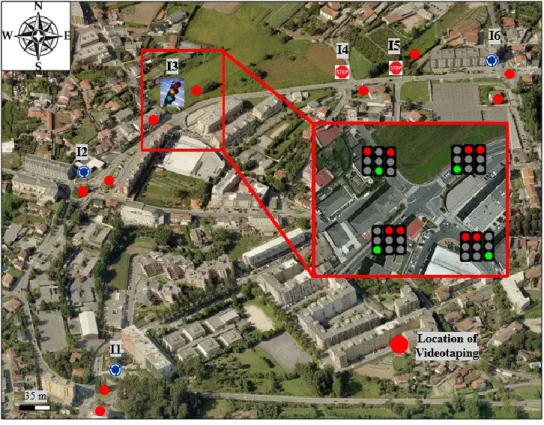
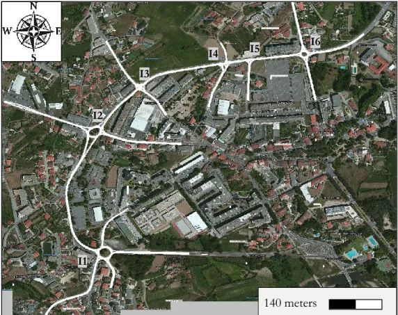
Thus, an urban mixed corridor with roundabouts/traffic lights/stop controlled junctions exhibiting high traffic was sought out for this research (Figure 2). The case study is located near the city of Guimarães (North of Portugal), a European medium-sized city with 158,124 inhabitants with a population density of 656 inhabitants/km2 _{(Statistics of Portugal, 2015).} The posted speed limit is 50 km/h and the corridor has one lane in each direction throughout its length. The spacing is not uniform between intersections (the coefficient of variation of average spacing is 0.58). The corridor is approximately 1,500 meters long, and it includes three single-lane roundabouts (I1/I2/I6), one traffic light intersection (I3), and two two-way stop controlled intersections (I4/I5). I3 has a fixed-cycle with the same setup during the day (overall cycle time is 107 seconds) and does not include any left-turn and right-turn lanes on entry legs. As noted, I2 and I3 are located in close proximity to each other (spacing of 167 meters). Table 1 presents the information regarding the site’s characteristics.

Figure 2 Aerial view of the selected corridor with the intersections’ identification (I1, I2, I3 – including phasing, I4, I5 and I6) (Guimarães, Portugal). Source:

https://www.bing.com/maps/

Table 1 Summary of the site characteristics.

3.2.2. Field Data Collection

During typical weekdays, traffic counts suggest that the evening peak period occurs between 5:30-7:00 p.m. Thus, the following data were collected at the selected corridor during that time in November and December 2014:

 Traffic flow (Light Passenger Vehicles – LPV, transit buses and Heavy Duty Vehicles – HDV);

 Time-Dependent Origin-Destination (O-D) matrices;  Traffic lights timing (cycle length and phasing);  Gap-acceptance and gap-rejection data;

 Queue lengths;

 High-resolution vehicle activity data (speed, acceleration/deceleration and grade). Traffic flows, queue lengths, and traffic lights timing were collected from overhead videos installed at strategic points along the corridor, as illustrated in Figure 2. With the exception of the I4 and I5 intersections, all entries were observed at each intersection to obtain the maximum queue length (for further information, please consult Table 4). The selection criterion was the existence of periods of continuous queuing on those locations. Traffic flows were recorded over 12 different typical weekdays (Tuesday and Wednesday) under dry weather conditions. Later, in the transportation laboratory, the traffic data for each vehicle class were compiled to define O-D tables based on trips along the whole corridor. Gap distributions data were also pulled out from the videotapes.

The vehicle activity data characterization were recorded using two LPVs with engine size lower than 1.4l (Euro III and Euro V Emission Standards) equipped with Global Positional System (GPS) travel record and On-Board Diagnostic (OBD), making several turning movements at the corridor (I1→I6 and I6→I1 directions, as displayed in Figure 2). It should be emphasized that the specifications of these vehicles are within the emissions’ factors of the emission model. Additionally, the test-vehicles are very representative of the LPV category in Europe (ICCT, 2014).

90 GPS travel runs for each through movement were performed for this study (approximately 150 km of road coverage over the course of 6 hours). To reduce systematic errors, 4 different drivers (three males and one female, ages 24 to 33 with varying levels of driving experience) performed an identical number of trips (approximately 18 each one) on each monitoring driving route. The above series of measurements were sufficient to enable the estimation of a 95% confidence interval in relation to the average and standard deviation of the measured parameters (Li et al., 2002).

3.2.3. Modeling corridor in VISSIM

The simulation model was run for 75 minutes (5:45-7:00 p.m.) with the first 15 minutes used as a warm-up period, and data extracted only for the remaining 60 minutes. Since transit buses and heavy-duty vehicles represented less than 1% of traffic composition, they were excluded from this analysis. Five O-D matrixes of 15 minutes for LPV were generated for the period between 5:45 p.m. and 7:00 p.m., and further imported in VISSIM. Traffic flows were assigned to respective route by applying Dynamic Traffic Assignment (DTA) (PTV, 2011).

The modeling of yield areas at roundabouts was made using the Priority Rules tool of the VISSIM model (PTV, 2011). For the purpose of analysis, the same minimum gap time and headway distance in each one of the yield areas was considered. The coded network is exhibited in Figure 3.

Figure 3 Coded network in VISSIM. Source: https://maps.google.com/

4. RESULTS

4.1. Model Calibration and Validation

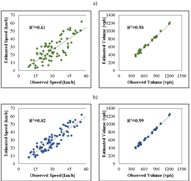
Using the initial default values, R-squared values of 0.98 and 0.61 were obtained from linear regression models between the estimated speeds and traffic flows, respectively, against field data, as displayed in Figure 4 a. After the calibration, (see Figure 4 b) the results demonstrated large improvements in speed values. The R-squared values for traffic flows and speed were higher than 0.80, indicating that the simulated data explained more than 80% variation in the observed data.

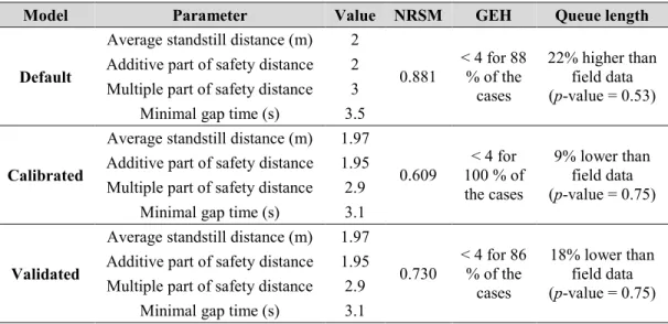
Table 2 presents the calibration and validation results for the traffic model and the corresponding statistic test. Since a fixed value was needed to setup the time resolution of traffic model and emission methodology (second-by-second), a constant value of 10 time steps per simulation seconds for simulation resolution parameter was used. After the calibration, all the links achieved a GEH less than 4, which fulfilled the calibration criteria (Dowling et al., 2004). The calibration results for calibrated gap time at roundabouts also reflected local driving habits (Vasconcelos et al., 2013). Regarding the validation results, the comparison of observed and estimated flows and travel time was conducted using 15 random seed runs (Hale, 1997), which demonstrated that 86% of the coded links attained GEH values below 4 (Dowling et al., 2004).

Figure 4 Observed vs. Estimated speed and traffic flows: a) Default parameters; b) Calibrated model.

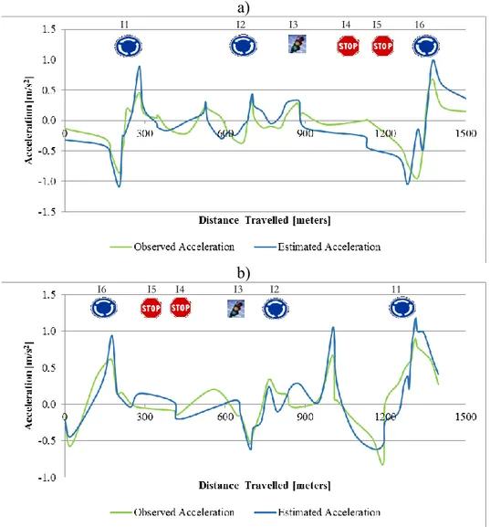
Figure 5 a-b exhibits the observed and estimated average acceleration profiles along the corridor for monitoring routes. The graphs confirmed that estimated acceleration values were slightly higher than observed data at the downstream intersections, which is in accordance with previous studies [e.g. (Fellendorf and Vortisch, 2010)]. Despite these differences, MAPE values did not exceed 20% in both routes, which suggested that the VISSIM calibrated parameters provided reasonable estimates for the studied corridor. Because vehicles were subject to continuous stop-and-go situations between downstream of I2 and upstream of I3, small variations of the acceleration curves were observed after I3 for I6-I1 route (Figure 5 b).

Figure 5 Observed and Estimated accelerations distributions along the corridor: a) I1-I6 route; b) I6-I1 route.

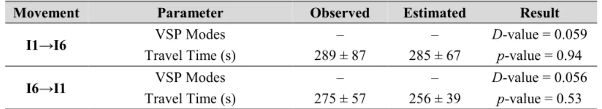
The assessment of VSP modes in terms of cumulative distributions revealed that two results from the observed and estimated data of the monitoring routes followed the same trend. In such cases, and as presented in Table 3, D-values for I1-I6 and I6-I1 routes with a 99% confidence level were 0.059 (D-critical = 0.060) and 0.056 (D-critical = 0.061), respectively. Still, the findings showed slight differences between travel time data samples (p-value >0.05). To conduct the above comparison approximately 15 data samples for each route were used.

Table 3 Summary of validation of traffic model for the monitoring routes.

4.2. Traffic performance results

Table 4 summarizes the simulated values of traffic flow on each approach intersection road during the one-hour evening peak (6:00-7:00 p.m.). The level‐of‐service (LOS) criteria, the queue distance and the volume/capacity (v/c) ratio for each lane are provided, as well as LOS criteria and stops per vehicle for the intersection (HCM, 2010). The average number of vehicles entering each intersection ranged from 1,060 to 2,590 vehicles per hour (vph) for I5 and I2, respectively.

Several conclusions about the effect of each intersection of the corridor can be drawn. First, I2 and I3 operate with poor levels of service, respectively, LOS E (control delay between 35 and 50 s/vehicle) and LOS D (control delay between 35 and 55 s/vehicle) (HCM, 2010). Second, the East entry of I2 and West entry of I3 reach queue distances exceeding 200 meters, which is longer than the available spacing between I2 and I3 (167 meters). In the eastbound route of I2, the queue exceeds 400 meters (almost the distance between the upstream of I3 and the downstream of I6, as presented in Table 1). This means that more than 50% of vehicles enter I2 from the East entry leg (~700 vph) are retained at the upstream of I3 (caused by red signal). Simultaneously, the through traffic (East-West and West-East) has to wait for left-turn vehicles since there are not left-turn lanes at I3.

The analysis of the corridor suggests that the main congestion focus is found at I3 influence area. Moreover, the short distance to the I2 paired with high traffic flows and an inefficient traffic control strategy, as is the case of I3, negatively affected overall corridor performance.

Replacing the current traffic control at I3 could be a solution to mitigate the traffic congestion for the studied corridor.

Table 4 Traffic performance results of the selected corridor

4.3. Operational Scenarios

With these concerns in mind, several scenarios were established to improve traffic performance and reduce vehicular emissions along the case study corridor. Initial evaluation performed in the simulation demonstrated that 130% of the traffic demand induced traffic congestion in the modelling network (several vehicles were retained in the centroids at the end of the simulation period).

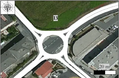
The baseline scenario is the calibrated simulation model with the existing control at the I3 intersection. Next, a single-lane roundabout layout (inscribed circle diameter = 33 m, circulating lane width = 5.6 m) replaced the traffic light (see Figure 6). The roundabout layout was designed according the Portuguese design guidelines (Bastos Silva and Seco, 2012). The latter two scenarios were analyzed and compared considering two main demand levels (see Table 5): (1) observed traffic flows (100% demand factor) and (2) expected traffic growth of 25% (125% demand factor).

Figure 6 Proposed single-lane roundabout layout at I3 intersection. Source: https://maps.google.com/

Table 5 Scenario description.

For each scenario, a fixed time signal control method was used at I3 together with the phase sequence exhibited in Figure 2. The cycle time and phase timing were optimized using aaSIDRA model (Akçelik, 2014) as follows:

 100% demand: East and West – 27 seconds; North – 12 seconds; South – 19 seconds (cycle length of 85 seconds);

 125% demand: East and West – 30 seconds; North – 12 seconds; South – 21 seconds (cycle length of 90 seconds).

To reflect the local car fleet composition, the total emissions were calculated considering the following distribution: 44% of GPV with engine size <1.2l; 35% of DPV<1.6l; and 21% of LDDT <2.5l (ACAP, 2014). Because the terrain was flat (slope <1%), the effect of the grade was ignored.

4.3.1. Traffic performance measures and emission rates

This section compares emissions and traffic performance parameters of the two scenarios to the baseline scenario and two demand levels (100% and 125%). The performance measures and vehicle activity data speed and acceleration/deceleration on a second-by-second basis (to be computed in the VSP methodology) were given from the vehicle record evaluation of the VISSIM model (PTV, 2011).

The emissions and traffic performance results are presented in Table 6 by scenario and demand level to the evening peak period (6:00-7:00 p.m.). Key observations from the data in Table 6 are:

 When the 100% demand factor level was considered, scenario 1 was the best design solution for I3 intersection. It had average emissions reductions of about 6%, while the average delay and number of stops decreased by more than 22%;

 For the 125% demand factor scenario, the difference in the amount of emissions between traffic light and single-lane roundabout increased, when compared with the observed demand levels. Scenario 1 yielded the highest emissions reductions in CO2 and HC with 24% and 27%, respectively. Alongside of each other, it was very effective in terms of traffic performance measures (its implementation allowed the total number of stops and average delay to be reduced by 60% and 44%, respectively);

 The average queue length on the entry legs of I2 and I3 decreased at scenario 1 when compared to the baseline scenario (57% and 64% short queues in 100% and 125% demand levels, respectively).

Table 6 Variation of emissions and traffic performance parameters per location in relation to the baseline scenario.

Another reason for increasing capacity after roundabout implementation may be due to the number of approaching vehicles at I2 and I3 (Table 7), especially under high demand levels. With 125% demand factor, the number of approaching vehicles at the I2 and I3 with baseline conditions was lower (-10%) than those obtained in the Scenario 1. This meant that I3 did not completely flow all traffic (even considering a longer green time along major arterials) that crossed the intersection. Accordingly, some vehicles no longer enter or leave other intersections, and further they are retained in the centroids. Table 7 also lists LOS criteria for the intersection. As suspected, LOS criteria at I2 and I3 improved after roundabout implementation. For instance, I2 operated with LOS C in both demand periods, which was not happened in the baseline (LOS E and LOC F for 100% and 125% demand factors, respectively).

It is worth noting that simulated left-turning vehicles delayed right-turning and through traffic behind them while waiting for a gap from opposing traffic at the I3 baseline. This phenomenon does not occur in the reality since some vehicles in the queue attempts to overtake the left-turning traffic if they have space on the road. However, left turning movements only represented 6% and 9% of westbound and eastbound approach traffic, respectively, at the I3 intersection.

Table 7 Number of approaching vehicles and LOS at the I2 and I3.

In summary, the comparison of the corridor’s layout dictated large improvements when a single-lane roundabout replaced the existing traffic light. This was particularly perceptible in the queue length, which was reduced by more than half. In the roundabout, vehicles do not always perform complete stops and a high proportion of vehicles are able to reach through its upstream areas. Despite the improvements, the average queue length is still high (>65 meters) in scenario 1, especially in a future traffic increase situation (125% demand factor). This presumably suggests that the spacing between I2 and I3 intersections could have an impact on the traffic operations along the corridor. This subject is addressed in the following section.

4.3.2. Multi-objective optimization

Considering the foregoing discussion, several spacing values were tested to find a set of optimal spacing locations between I2 and I3 that allowed minimizing delay and vehicular emissions. Scenario 1 with 100% and 125% demand levels was then applied, assuming several spacing lengths (S) ranging from 70 meters to 250 meters in 10-meters increments relatively to the I2 exit section. For these two demand levels, the roundabout I3 was moved along the mid-block section within feasible values (according to the geometry layout of the corridor). It should be noted that the distance to downstream intersection (I4) is only 253 meters, as described in Table 1.

The following objective variables were optimized: 1) delay versus CO2; 2) delay versus CO; 3) delay versus NOX and 4) delay versus HC. Several regression models were tested to fit each variable against the decision variable (S). A set of 10 optimal spacing solutions was used in this research.

As solution for the proposed problem, a genetic algorithm (GA) was selected. GAs are heuristic search techniques based on the evolutionary ideas of natural selection and genetics (Sivanandam and Deepa, 2007). The Fast-Non-Dominated Sorting Genetic Algorithm (NSGA-II) proposed by Deb et al. (2002) was used. NSGA-II proceed in four main steps. First, the population (optimal spacing length values) was initialized taken into account the objective variables (delay, CO, CO2, NOX or HC) range and spacing constraints (distance in relation to the downstream I4).

Second, the population was sorted based on a non-domination criteria (a feasible solution is non-dominated whether does not exist another feasible solution better than the actual one as a delay value without worsening CO, CO2, NOX or HC values). NSGA-II uses a binary tournament selection based on the rank and crowding distance process for choosing the parents from the population. An individual (S value) is selected in the rank if is smaller than the other individual or if crowding distance is greater than the other. The crowding distance measures how close an individual is to its neighbors. The diversity in the final optimal spacing solutions is better as the crowding distance is larger.

In the third step, the selected population generated offspring by applying crossover and mutation rates, and then parents and offspring merged to select the best individuals in the population. This allows preserving individuals from one generation to another (elitism). Four, the procedure stopped after reaching stopping criteria (number of generations/iterations), and the optimal solutions found in the Pareto Approximate Front (POF). Deb et al. (2002) details the overview of NSGA-II.

To ensure the diversity in the solutions and the convergence to Pareto Optimal Front (POF) (Konak et al., 2006), a sensitivity analysis was conducted. First, the maximum number of iterations (stopping criteria) was set to 2000 for all the test instances, while the crossover and mutation rates were set at 90% and 10%, respectively. Second, each scenario was run 15 times in the NSGA-II code. In doing so, the indicators measured the diversity of the solutions [Spread and Uniformity Measure metrics (Deb, 2001)] and the convergence to POF (number of dominated solutions) were computed and analyzed. Once guaranteed the above objectives (diversity and convergence) in all scenarios, an equal maximum number of generations was used.

The analysis of the diversity in the solutions and convergence to POF dictated that a maximum of 500 iterations were sufficient to reach convergence. After testing several crossover and mutation rates, a slight variation of the final POF was observed on each of the multi-objective runs. Thus, crossover and mutation rates were set at 95% and 5%, respectively.

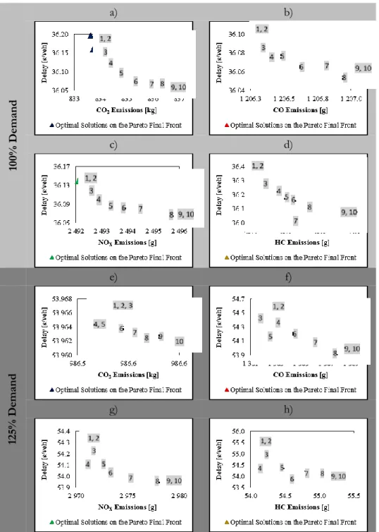
Figure 7 depicts the final Pareto front from the final populations obtained for Scenario 1 and the average corridor v/c ratio. For each demand level, a 2-D scatter plot with two objective functions – emissions (x-axis), and average delay (y-axis) – is illustrated. Each data label is a Pareto point that represents an optimal spacing (S) solution of the final POF (its correspondent value is presented in Table 8). The optimal spacing solutions, which conducted with the minimal vehicular emissions, were allocated furthers to the upper-left, while the optimal spacing solutions, which led to the minimal average delay, was assigned lower-right. A trade-off occurs along the graph of the optimal spacing solutions.

For the 100% demand factor level (Figure 7 a-d), the findings confirmed that low-spacing values (<180 meters) and high-spacing values (>222 meters) were not good options. Furthermore, no significant differences in the optimal spacing set among pollutants were observed. For solution 5 (data label point which is closest to the abscissa of the graph), that is, 207 meters of spacing, average delay and CO2 emissions decreased by 5% and 2%, respectively, when compared to the existing spacing. For a chosen value of the lowest optimal spacing value (solution 1), reductions of 3%, 2%, 4% and 6% in CO2, CO, NOX and HC, respectively, can be expected on case study corridor in relation to 167 meters of spacing (see Table 6 for those details).

Concerning the highest demand level (125%), the final Pareto front for all pollutants pointed out that high-spacing (>220 meters) must be avoided by transportation planners to implement at the case study corridor (Figure 7 e-h). For instance, if one adopted solution 6 (intermediate solution), then one could save up to 3%, 7% and 8% in CO, NOX and HC, respectively. Alternatively, a decision-maker can use a spacing solution of 200 meters, and reduce the average amount of emissions and delay in more than 5% and 6%, respectively, if the spacing was 167 meters (actual location). However, the set of final POF varied for some pollutants. Specifically, optimal spacing values for CO2 ranged from 199 meters and 203 meters, while

local pollutants accepted spacing values close to the actual spacing distance (~180 meters). This is mostly because of the high acceleration/deceleration rates that vehicles experience as they approach each intersection, and the result is especially relevant for CO emissions.

Figure 7 The approximate Pareto front for scenario 1 under different traffic conditions: 100% demand factor (a, b, c and d) and 125% demand factor (e, f, g and h). Table 8 Solution lists of the spacing values for the scenario 1 considering objective

function criteria. 4.4. Policy Implications

The findings confirm that spacing of roundabouts ranging from 180 to 222 meters achieves moderate improvements in both delay and emissions of the corridor when compared to a low distance value. This means that the current spacing (~167 meters) does not completely optimize traffic operations along the corridor. The location of the intersection in further distances (high spacing) is a constraint for the downstream intersections. This is especially true under high traffic demand levels.

The optimal spacing values obtained in this paper were much lower than those suggested by several guidelines (FHWA, 2013; Gluck et al., 1999; TRB, 2003), which were based on American study-cases. Conversely, some of the optimal spacing values were close to those recommended by European guidelines (SETRA, 2002). The findings also confirmed that the spacing has a great impact on vehicle delay and emissions along the corridor, as mentioned by a previous research (Fernandes et al., 2015b).

Hence, an assessment of a hot spot traffic segment of a given corridor must be carefully done. This includes a proper traffic control implementation together with an optimization of spacing design according to the location-specific operational or emission needs. Moreover, in terms of policy implications, such design criteria should not be centered only to improve traffic performance or to reduce global pollutants as CO2. It must be taken into account which major environmental concerns in a certain region are presented (for instance to reduce NOX and HC pollution levels).

It is well-known that the rapid growth of cities has strained the capacity to provide satisfactory levels of service such as transportation, education, or sanitation (Bhatta, 2010). Transportation planning is currently being challenged with a broader planning view (Miranda and Rodrigues da Silva, 2012). The lack of consistent and well-experimented planning policies has contributed to the urban sprawl phenomenon in many countries. Therefore, a mixed land-use policy with a suitable transportation design strategy is essential to fight against sprawl as well as to maintain or improve overall network performance. Focusing on the transportation sector, several other strategies may be developed, such as policies and incentives for encouraging the use of public transportation systems (UITP, 2014), implementation of traffic restriction measures on urban areas (Fernandes et al., 2014) or introduction of low emission zones (Low Emission Zones in Europe Network, 2013). It should be mentioned that the simple analysis segment of the corridor does not solve all issues associated with inefficient urban planning per se. Nonetheless, if overall network

performance is improved, the utility of spacing as a policy management measure on urban areas can be considered.

5. CONCLUSIONS

This research analyzed a specific segment of an urban corridor with closely-spaced intersections (single-lane roundabout and traffic light spaced approximately 167 meters), which presented weak traffic performance and environmental levels. To mitigate these issues, the traffic light was replaced by a single-lane roundabout, and the results were compared with the existing situation under different demand levels (actual traffic and an expected traffic growth of 25%). The paper also performed an optimization analysis for the best traffic control by varying the spacing between those intersections with the main purpose of improving delay and CO2, CO, NOX and HC vehicular emissions. The analysis was based on a microsimulation approach, using a traffic model integrated with an emission methodology. As a solution algorithm, NSGA-II was used to search the optimal solutions for the proposed problem.

The methodology of this paper can be outlined in the following steps: 1) To identify a highly-congested specific segment of a given corridor that has a great impact on the traffic operations; 2) To understand the causes that led to the inefficient operational and emissions levels of such segment; 3) To implement and compare different traffic control treatments to improve traffic performance and emissions outcomes; 4) To select its suitable and feasible (taking into account corridor-specific needs) location in relation to downstream and upstream intersections, for the best traffic control; 5) To define whether there is a need to fulfill the emissions’ levels for a specific pollutant during the optimization of the spacing between intersections.

The following findings were obtained for the actual traffic demand:

 Single-lane roundabout led to the lowest number of vehicle stops, 24% less average delay and 57% less queue length; Also, it was environmentally better than the traffic light traffic control solution (5-7%, depending on the pollutant);

 For the above traffic control, an additional decrease of emissions of 6% may be expected by adopting an optimized spacing of about 207 meters from an upstream roundabout when compared to the existing spacing.

The following findings were found in future expected demand level:

 Single-lane roundabout yielded emissions than traffic light (16-27%, depending on the pollutant), and delay and queue length were shortened by 44% and 64%, respectively;

 The optimal spacing for CO2 range from 199 to 204 meters, while spacing values for local pollutants of approximately 180 meters can be adopted. Considering a spacing value of 200 meters, vehicular emissions and average delay were predicted to be reduced in more than 5 and 6%, respectively when compared to the existing spacing. Overall, the variation of delay and different pollutant emissions pointed to the moderate impact of spacing on delay and emissions along corridors using the proper traffic control strategy.

ACKNOWLEDGMENTS

The authors acknowledge to Toyota Caetano Portugal, which allowed the use of vehicles and to the volunteers that participated in the data collection. P. Fernandes acknowledges the support of FCT Scholarship SFRH/BD/87402/2012. The authors also acknowledge to the project PTDC/EMS-TRA/0383/2014 (that was funded within the project 9471-Reiforcement of RIDTI and funded by FEDER fundos), to the Strategic Project UID/EMS/00481/2013-FCT and CENTRO- 01-0145-FEDER-022083.

REFERENCES

ACAP, 2014. Automobile Industry Statistics 2013 Edition. ACAP – Automobile Association of Portugal. Akçelik, R., 2014. Modeling Queue Spillback and Nearby Signal Effects in a Roundabout Corridor, 4th International Roundabout Conference, Transportation Research Board, Seattle, WA, United States.

Anya, A.R., Rouphail, N.M., Frey, H.C., Liu, B., 2013. Method and Case Study for Quantifying Local Emissions Impacts of Transportation Improvement Project Involving Road Realignment and Conversion to Multilane Roundabout, Transportation Research Board 92nd Annual Meeting, Washington, DC.

Association, A.P., Steiner, F.R., Butler, K., 2012. Planning and Urban Design Standards. John Wiley & Sons, New York, US.

Bared, J.G., Edara, P.K., 2005. Simulated Capacity of Roundabouts and Impact of Roundabout Within a Progressed Signalized Road, Transportation Research Board National Roundabout Conference, Vail, Colorado.

Barth, M., Boriboonsomsin, K., 2012. ECO-ITS: Intelligent Transportation System Applications to Improve Environmental Performance, Federal Highway Administration, FHWA-JPO-12-042, U.S. Department of Transportation, Washington, DC.

Bastos Silva, A., Seco, Á.J.M., 2012. Dimensionamento de Rotundas-Disposições Normativas [In Portuguese], Instituto de Infra-Estruturas Rodoviárias, Lisbon, Portugal.

Bhatta, B., 2010. Analysis of Urban Growth and Sprawl from Remote Sensing Data. Springer.

Bugg, Z., Schroeder, B., Jenior, P., Brewer, M., Rodegerdts, L., 2015. A Methodology to Compute Roundabout Corridor Travel Time, Transportation Research Board 94th Annual Meeting, Washington, DC.

Chevallier, E., Can, A., Nadji, M., Leclercq, L., 2009. Improving noise assessment at intersections by modeling traffic dynamics. Transportation Research Part D: Transport and Environment 14(2), 100-110.

Coelho, M.C., Farias, T.L., Rouphail, N.M., 2006. Effect of roundabout operations on pollutant emissions. Transportation Research Part D: Transport and Environment 11(5), 333-343.

Coelho, M.C., Farias, T.L., Rouphail, N.M., 2009a. A Numerical Tool for Estimating Pollutant Emissions and Vehicles Performance in Traffic Interruptions on Urban Corridors. International Journal of Sustainable Transportation 3(4), 246-262.

Coelho, M.C., Frey, H.C., Rouphail, N.M., Zhai, H., Pelkmans, L., 2009b. Assessing methods for comparing emissions from gasoline and diesel light-duty vehicles based on microscale measurements. Transportation Research Part D: Transport and Environment 14(2), 91-99.

Deb, K., 2001. Multi-Objective Optimization Using Evolutionary Algorithms. John Wiley & Sons, New York, US.

Deb, K., A. Pratap, S. Agarwal, Meyarivan, T., 2002. A fast and elitist multiobjective genetic algorithm: NSGA-II. Evolutionary Computation, IEEE Transactions on Evolutionary Computation 6(2), 182-197.

Dowling, R., Skabadonis, A., Alexiadis, V., 2004. Traffic analysis toolbox, volume III: Guidelines for applying traffic microsimulation software, Federal Highway Administration, FHWA-HRT-04-040, U.S. Department of Transportation, Washington, DC.

EEA, 2006. Urban sprawl in Europe - The ignored challenge European Environment Agency, EEA Report No 10/2006, Copenhagen, Denmark.

Fellendorf, M., Vortisch, P., 2010. Microscopic Traffic Flow Simulator VISSIM, In: Barceló, J. (Ed.), Fundamentals of Traffic Simulation. Springer New York, pp. 63-93.

Fernandes, P., Bandeira, J.M., Fontes, T., Pereira, S.R., Schroeder, B.J., Rouphail, N.M., Coelho, M.C., 2014. Traffic Restriction Policies in an Urban Avenue: A Methodological Overview for a Trade-Off Analysis of Traffic and Emission Impacts Using Microsimulation. International Journal of Sustainable Transportation, in press.

Fernandes, P., Fontes, T., Neves, M., Pereira, S.R., Bandeira, J.M., Coelho, M.C., Rouphail, N.M., 2015a. Assessment of corridors with different types of intersections: An environmental and traffic performance analysis. Journal of Transportation Research Record: Journal of the Transportation Research Board 2503(-1), 39-50.

Fernandes, P., Salamati, K., Coelho, M.C., Rouphail, N.M., 2015b. Identification of the Emission Hotspots in Roundabouts Corridors. Transportation Research Part D: Transport and Environment 37, 48-64.

FHWA, 2013. Signalized Intersections: An Informational Guide, Federal Highway Administration, FHWA-SA-13-027, U.S. Department of Transportation, Washington, DC.

Fontes, T., Fernandes, P., Rodrigues, H., Bandeira, J.M., Pereira, S.R., Khattak, A.J., Coelho, M.C., 2014. Are HOV/eco-lanes a sustainable option to reducing emissions in a medium-sized European city? Transportation Research Part A: Policy and Practice 63, 93-106.

Fwa, T.F., 2005. The Handbook of Highway Engineering. CRC Press, London, UK.

Gluck, J., Levinson, H.S., Stover, V., 1999. Impacts of Access Management Techniques, NCHRP Report 420, Transportation Research Board, Washington, DC.

Guerrieri, M., Corriere, F., Lo Casto, B., Rizzo, G., 2015. A model for evaluating the environmental and functional benefits of “innovative” roundabouts. Transportation Research Part D: Transport and Environment 39, 1-16.

Guo, R., Zhang, Y., 2014. Exploration of correlation between environmental factors and mobility at signalized intersections. Transportation Research Part D: Transport and Environment 32, 24-34.

Hale, D., 1997. How many netsim runs are enough? McTrans 11(3), 1-9.

Hallmark, S., Fitzsimmons, E., Isebrands, H., Giese, K., 2010. Roundabouts in Signalized Corridors. Transportation Research Record: Journal of the Transportation Research Board 2182, 139-147.

Hallmark, S., Wang, B., Mudgal, A., Isebrands, H., 2011. On-Road Evaluation of Emission Impacts of Roundabouts. Transportation Research Record: Journal of the Transportation Research Board 2265, 226-233.

HCM, 2010. The Highway Capacity Manual, Transportation Research Board, Washington, DC.

ICCT, 2014. European Vehicle Market Statistics Pocketbook 2014, ICCT – The International Council on Clean Transportation, Berlin, Germany.

Isebrands, H., Hallmark, S., Fitzsimmons, E., Stroda, J., 2008. Toolbox to Evaluate the Impacts of Roundabouts on a Corridor or Roadway Network, Publication MN/RC 2008-24, Minnesota Department of Transportation, Research Services Section, St. Paul, MN.

Konak, A., Coit, D.W., Smith, A.E., 2006. Multi-objective optimization using genetic algorithms: A tutorial. Reliability Engineering & System Safety 91(9), 992-1007.

Krogscheepers, J., Watters, M., 2014. Roundabouts along Rural Arterials in South Africa, Transportation Research Board 93rd Annual Meeting, Washington, DC.

Kutz, M., 2008. Environmentally Conscious Transportation, John Wiley & Sons, New York, US.

Kwak, J., Park, B., Lee, J., 2012. Evaluating the impacts of urban corridor traffic signal optimization on vehicle emissions and fuel consumption. Transportation Planning and Technology 35(2), 145-160.

Li, S., Zhu, K., van Gelder, B., Nagle, J., Tuttle, C., 2002. Reconsideration of Sample Size Requirements for Field Traffic Data Collection with Global Positioning System Devices. Transportation Research Record: Journal of the Transportation Research Board 1804, 17-22.

Low Emission Zones in Europe Network, 2013. Low Emission Zones in Europe. Europe-wide Information on LEZs, http://lowemissionzones.eu [Accessed June 2015].

Miranda, H.d.F., Rodrigues da Silva, A.N., 2012. Benchmarking sustainable urban mobility: The case of Curitiba, Brazil. Transport Policy 21, 141-151.

Mudgal, A., Hallmark, S., Carriquiry, A., Gkritza, K., 2014. Driving behavior at a roundabout: A hierarchical Bayesian regression analysis. Transportation Research Part D: Transport and Environment 26, 20-26. Newman, P., Jennings, I., 2012. Cities as Sustainable Ecosystems: Principles and Practices. Island Press, Washington, DC.

Nicoli, F., Pratelli, A., Akçelik, R., 2015. Improvement Of The West Road Corridor For Accessing The New Hospital Of Lucca (Italy). WIT Transactions on The Built Environment 146, 449-460.

Park, B., Yun, I., Ahn, K., 2009. Stochastic Optimization for Sustainable Traffic Signal Control. International Journal of Sustainable Transportation 3(4), 263-284.

PTV, 2011. Vissim 5.30-05 user manual, In: Planung Transport Verkehr AG, K., Germany (Ed.).

SETRA, 2002. The design of interurban intersections on major roads, Service d'Etudes Techniques des Routes et Autoroutes Centre de la Sécurité et des Techniques Routières, Bagneux Cedex, France.

Sivanandam, S.N., Deepa, S.N., 2007. Introduction to Genetic Algorithms. Springer Berlin Heidelberg. Statistics of Portugal, 2015. Censos 2011 [In Portuguese] http://mapas.ine.pt/map.phtml [Accessed March 2015].

Tarko, A.P., Inerowicz, M., Lang, B., 2008. Safety and Operational Impacts of Alternative Intersections: Volume I, Federal Highway Administration, FHWA/IN/JTRP-2008/23, U.S. Department of Transportation, Washington, DC.

Tollazzi, T., Tesoriere, G., Guerrieri, M., Campisi, T., 2015. Environmental, functional and economic criteria for comparing “target roundabouts” with one- or two-level roundabout intersections. Transportation Research Part D: Transport and Environment 34, 330-344.

TRB, 2003. Access Management Manual, Transportation Research Board Committee on Access Management, National Research Council, Washington, DC.

UITP, 2014. The Rising Importance of Energy Efficiency in Urban Transport, http://www.uitp.org/rising-importance-energy-efficiency-urban-transport [Accessed June 2015].

UN, 2014. World Urbanization Prospects - The 2014 Revision, United Nations, ST/ESA/SER.A/352, New York, US.

USEPA, 2002. Methodology for developing modal emission rates for EPA’s multi-scale motor vehicle & equipment emission system, Prepared by North Carolina State University for US Environmental Protection Agency, EPA420, Ann Arbor, MI.

Várhelyi, A., 2002. The effects of small roundabouts on emissions and fuel consumption: a case study. Transportation Research Part D: Transport and Environment 7(1), 65-71.

Vasconcelos, L.P., A. M. Seco, A. B. Silva., 2013. Comparison of procedures to estimate critical headways at roundabouts. Promet –Traffic&Transportation 25(1), 43-53.

Xia, H., Boriboonsomsin, K., Barth, M., 2012. Dynamic Eco-Driving for Signalized Arterial Corridors and Its Indirect Network-Wide Energy/Emissions Benefits. Journal of Intelligent Transportation Systems 17(1), 31-41.

Zhai, H., Frey, H.C., Rouphail, N.M., 2008. A Vehicle-Specific Power Approach to Speed- and Facility-Specific Emissions Estimates for Diesel Transit Buses. Environmental Science & Technology 42(21), 7985-7991.

Figure 8 Summary of methodological steps. Field Data collection

Microsimulation platform of traffic (VISSIM) and emissions (VSP)

Calibrated Model

Vehicle Activity Operational

Scenarios

Model Outputs _Methodology VSP

Figure 9 Aerial view of the selected corridor with the intersections’ identification (I1, I2, I3 – including phasing, I4, I5 and I6) (Guimarães, Portugal). Source:

Figure 10 Coded network in VISSIM. Source: https://maps.google.com/ 140 meters I1 I2 I3 I4 I5 I6

a)

b)

Figure 11 Observed vs. Estimated speed and traffic flows: a) Default parameters; b) Calibrated model.

a)

b)

Figure 12 Observed and Estimated accelerations distributions along the corridor: a) I1-I6 route; b) I6-I1 route.

I1 I2 I3 I4 I5 16

Figure 13 Proposed single-lane roundabout layout at I3 intersection. Source: https://maps.google.com/

20 m I3

100 % Dem and a) b) c) d) e) f) 125 % Dem and g) h)

Note: v/c is the average volume-to-capacity ratio with optimized traffic conditions

Figure 14 The approximate Pareto front for scenario 1 under different traffic conditions: 100% demand factor (a, b, c and d) and 125% demand factor (e, f, g and h).

v/c ≈ 0.86 _{v/c ≈ 0.86}

v/c ≈ 0.86 v/c ≈ 0.86

v/c ≈ 0.79 v/c ≈ 0.79

Table 9 Summary of the site characteristics. Intersection ID Type coordinates GPS # approach lanes # legs Distance to downstream analysis intersection [m] Average Spacing [m] I1 _Roundabout Single-lane 41°28'58.62"N _8°21'7.92"W 1 5 453 223.4 I2 _Roundabout Single-lane 41°29'11.09"N _8°21'9.17"W 2 4 167 I3 Traffic Light 41°29'15.75"N _8°21'3.68"W 1 4 253 I4 _Controlled Stop- 41°29'18.18"N _{8°20'53.20"W} 1 3 70 I5 _Controlled Stop- 41°29'18.56"N _{8°20'50.23"W} 1 3 174 I6 _Roundabout Single-lane 41°29'19.12"N _{8°20'43.75"W} 1 4 -

Table 10 Summary of calibration and validation of traffic model.

Model Parameter Value NRSM GEH Queue length

Default

Average standstill distance (m) 2

0.881 < 4 for 88 % of the cases

22% higher than field data (p-value = 0.53) Additive part of safety distance 2

Multiple part of safety distance 3 Minimal gap time (s) 3.5

Calibrated

Average standstill distance (m) 1.97

0.609 100 % of < 4 for the cases

9% lower than field data (p-value = 0.75) Additive part of safety distance 1.95

Multiple part of safety distance 2.9 Minimal gap time (s) 3.1

Validated

Average standstill distance (m) 1.97

0.730 < 4 for 86 % of the cases

18% lower than field data (p-value = 0.75) Additive part of safety distance 1.95

Multiple part of safety distance 2.9 Minimal gap time (s) 3.1

Table 11 Summary of validation of traffic model for the monitoring routes.

Movement Parameter Observed Estimated Result

I1→I6 VSP Modes – – D-value = 0.059

Travel Time (s) 289 ± 87 285 ± 67 p-value = 0.94

I6→I1 VSP Modes – – D-value = 0.056

Travel Time (s) 275 ± 57 256 ± 39 p-value = 0.53

Table 12 Traffic operational data of the selected corridor

ID

North Approach South Approach West Approach East Approach

Average LOS Stops per veh Traffic flow [vph] L O S Queue (m) v/c ratio Traffic flow [vph] L O S Queue (m) v/c ratio Traffic flow [vph] L O S Queue (m) v/c ratio Traffic flow [vph] L O S Queue (m) v/c ratio I1 276 D 65 0.70 654 F 251 1.03 797 C 175 0.92 640 C 92 0.76 C 1.33 I2 684 C 134 0.86 291 C 49 0.60 904 F 291 1.10 703 F 440 1.21 E 1.88 I3 114 E 56 0.47 348 E 108 0.73 491 D 203 0.57 526 D 212 0.75 D 0.86 I4 21 C 3 0.09 21 C 3 0.07 509 A 24 0.27 513 A 24 0.28 C 0.06 I5 - - - - 48 C 11 0.14 514 A 0 0.28 495 A 24 0.27 D 0.13 I6 256 B 29 0.45 251 B 21 0.36 403 B 37 0.52 606 B 68 0.68 B 0.83

Note: * The Southwest approach of I1 was excluded (traffic flows<20 vph); ** Based on preliminary traffic analysis with assignment of the overall corridor

Table 13 Scenario Description.

Scenario Traffic Control at I3 intersection Demand _Level

Baseline Traffic Light 100%

125%

Scenario 1 Single-lane Roundabout 100%

Table 14 Variation of emissions and traffic performance parameters per location in relation to the baseline scenario.

Demand

Level Scenario

Emissions Traffic Performance

CO2

[kg] CO [g] NO

X

[g] HC [g] [s/veh] Delay Total stops lengthQueue a _[m]

100% Baseline 903 1291 2767 48 50.19 5869 154 Scenario 1 _(-6%) 848 _(-5%) 1222 _(-7%) 2584 _(-5%) 46 _(-24%) 38.05 _(-23%) 4542 _(-57%) 66 125% Baseline 1363 1698 4016 81 103.67 18804 325 Scenario 1 _(-24%) 1033 _(-16%) 1432 _(-20%) 3199 _(-27%) 59 _(-44%) 58.16 _(-60%) 7611 _(-64%) 116 Note: a Average queue length at the I2/I3 entry legs

Table 15 Number of approaching vehicles and LOS at the I2 and I3.

Scenario Demand

level ID Traffic [vph] Approach Average LOS

Baseline 100% I3 2,505 E I4 1,403 D 125% I3 2,241 F I4 1,268 F Scenario 1 100% I3 2,507 C I4 1,407 A 125% I3 2,712 C I4 1,806 C

Table 16 Solution lists of the spacing values for the scenario 1 considering objective function criteria. Dema nd Level Solut ion

Delay vs CO2 Delay vs CO Delay vs NOX Delay vs HC

Spaci ng [m] Dela y [s/ve h] CO 2 [kg ] Spaci ng [m] Dela y [s/ve h] CO [g] Spaci ng [m] Dela y [s/ve h] NO X [g] Spaci ng [m] Dela y [s/ve h] H C [g] 100% 1 196 36.2 833 .6 207 36.1 1206.3 202 36.1 2492.1 181 36.4 43.4 2 196 36.2 833 .6 207 36.1 1206.3 202 36.1 2492.1 181 36.4 43.4 3 200 36.2 833 .7 209 36.1 1206.3 205 36.1 2492.3 184 36.3 43.4 4 203 36.1 833 .9 210 36.1 120 6.3 207 36.1 249 2.5 193 36.2 43.5 5 207 36.1 834 .3 212 36.1 1206.4 209 36.1 2492.9 199 36.2 43.6 6 211 36.1 834 .8 213 36.1 1206.5 212 36.1 2493.6 202 36.1 43.6 7 214 36.1 835 .4 216 36.1 1206.8 213 36.1 2494.0 203 36.1 43.6 8 217 36.1 836 .1 217 36.1 1206.9 217 36.1 2495.3 207 36.1 43.7 9 218 36.1 836 .2 218 36.1 120 7.0 218 36.1 249 5.7 218 36.1 43.9 10 218 36.1 836 .2 218 36.1 1207.0 218 36.1 2495.7 218 36.1 43.9 125% 1 199 53.9 6 986.6 181 54.6 1382.0 183 54.4 2970.7 184 55.6 54.1 2 199 53.9 6 986 .6 181 54.6 138 2.0 183 54.4 297 0.7 184 55.6 54.1 3 199 53.9 6 986.6 184 54.5 1382.1 187 54.3 2970.9 188 55.2 54.1 4 200 53.9 6 986.6 189 54.4 1382.3 189 54.2 2971.3 191 54.8 54.2 5 200 53.9 6 986.6 190 54.3 1382.6 191 54.1 2971.7 198 54.5 54.3 6 201 53.9 6 986.6 193 54.1 1384.1 193 54.1 2972.4 205 54.1 54.7 7 201 53.9 7 986 .6 196 54.0 138 5.7 200 54.0 297 5.3 210 54.0 54.8 8 202 53.9 7 986.6 202 54.0 1387.4 204 54.0 2977.5 212 54.0 55.0 9 203 53.9 7 986.6 204 54.0 1387.9 206 54.0 2978.7 215 54.0 55.1 10 203 53.9 7 986.6 204 54.0 1387.9 206 54.0 2978.7 215 54.0 55.1