The impact of traffic emissions on atmospheric ozone and OH: results from QUANTIFY

(1)

ACPD

8, 18219–18266, 2008

Tra_ffic emissions: impact on ozone and

OH

P. Hoor et al.

Title Page

Abstract Introduction

Conclusions References

Tables Figures

◭ ◮

Back Close

Full Screen / Esc

Printer-friendly Version

Interactive Discussion Atmos. Chem. Phys. Discuss., 8, 18219–18266, 2008

www.atmos-chem-phys-discuss.net/8/18219/2008/ © Author(s) 2008. This work is distributed under the Creative Commons Attribution 3.0 License.

Atmospheric Chemistry and Physics Discussions

This discussion paper is/has been under review for the journalAtmospheric Chemistry

and Physics (ACP). Please refer to the corresponding final paper inACPif available.

The impact of tra

_ffi

c emissions on

atmospheric ozone and OH: results from

QUANTIFY

P. Hoor1, J. Borken-Kleefeld2, D. Caro3, O. Dessens4, O. Endresen5, M. Gauss6, V. Grewe7, D. Hauglustaine3, I. S. A. Isaksen6, P. J ¨ockel1, J. Lelieveld1,

E. Meijer8, D. Olivie9, M. Prather10, C. Schnadt Poberaj11, J. Staehelin11, Q. Tang10, J. van Aardenne12, P. van Velthoven8, and R. Sausen7

1

Max Planck Institute for Chemistry, Department of Atmospheric Chemistry, 55020 Mainz, Germany

2

Transportation Studies, German Aerospace Center (DLR), Berlin, Germany

3

Laboratoire des Sciences du Climat et de l’Environment (LSCE), CEN de Saclay, Gif-sur-Yvette, France

4

Centre for Atmospheric Science, Department of Chemistry, Cambridge, UK

5

DNV, Det Norske Veritas (DNV), Oslo, Norway

6

Department of Geosciences, University of Oslo, Norway

7

(2)

ACPD

8, 18219–18266, 2008

OH

P. Hoor et al.

Title Page

Tables Figures

◭ ◮

Back Close

Full Screen / Esc

Interactive Discussion

8

Royal Netherlands Meteorological Institute, KNMI, De Bilt, The Netherlands

9

Meteo France, CNRS, Toulouse, France

10

Department of Earth System Science, University of California, Irvine, USA

11

Institute for Atmospheric and Climate Science, Swiss Federal Institute of Technology, Z ¨urich, Switzerland

12

Joint Research Center, JRC, Ispra, Italy

Received: 9 July 2008 – Accepted: 1 September 2008 – Published: 21 October 2008

Correspondence to: P. Hoor ([email protected])

(3)

ACPD

8, 18219–18266, 2008

OH

P. Hoor et al.

Title Page

Tables Figures

◭ ◮

Back Close

Full Screen / Esc

Abstract

To estimate the impact of emissions by road, aircraft and ship traffic on ozone and OH

of the present-day atmosphere seven different atmospheric chemistry models

simu-lated the atmospheric composition of the year 2003. Based on newly developed global emission inventories for road, maritime and aircraft emission data sets each model 5

performed a series of five simulations: A base scenario using the full set of emissions, three sensitivity studies with each individual sector of transport reduced by 5% and one

simulation with all traffic related emissions reduced by 5%. The approach minimizes

non-linearities in atmospheric chemical effects and are later scaled to 100%.

The global annual mean impact of ship emissions on ozone in the boundary layer 10

leads to an increase of ozone of 1.2%, followed by road (0.87%) and aircraft emissions

(0.3%). In the upper troposphere between 200–300 hPa both road and ship traffic affect

ozone by 1.1%, whereas aircraft emissions contribute 0.9%. However, the sensitivity

of ozone formation per NO_xmolecule emitted is highest for aircraft exhausts.

The local maximum effect of the summed traffic emissions on the ozone column

pre-15

dicted by the models is 4.0 DU and occurs over the northern subtropical Atlantic. The

impact of tra_ffic emissions on total ozone in the Southern Hemisphere is approximately

half of the northern hemispheric perturbation.

Below 800 hPa both ozone and OH respond most sensitively to ship emissions in

the marine boundary layer over the Atlantic, where the e_ffect can exceed 10% (zonal

20

mean) which is 80% of the total traffic induced ozone perturbation. In the Southern

Hemisphere ship emissions contribute relatively strongly to the total ozone perturba-tion by 60%–80% throughout the year (equivalent to 1–1.5 ppbv).

Road emissions have the strongest impact on ozone in the continental boundary layer

and the free troposphere in summer. They also affect the upper troposphere

particu-25

larly during northern summer associated with strong convection in mid latitudes. Ozone

perturbations due to road traffic show the strongest seasonal cycle in the northern

(4)

ACPD

8, 18219–18266, 2008

OH

P. Hoor et al.

Title Page

Tables Figures

◭ ◮

Back Close

Full Screen / Esc

The OH concentration in the boundary layer is most strongly affected by ship

emis-sions, which has a significant influence on the lifetime of many trace gases including methane. Methane lifetime changes due to ship emissions amount to 4.1%, followed by road (1.6%) and air traffic (1.0%).

1 Introduction

5

The rise in energy consumption by the growing human population and the increasing mobility are associated with emissions of air pollutants in particular by road and air

traffic as well as international shipping. These emissions are expected to increase

in future, affecting air quality and climate (Kahn Ribeiro et al., 2007) and vice versa

(Hedegaard et al., 2008). The impact of air traffic emissions has been subject of

vari-10

ous investigations (e.g. Hidalgo and Crutzen, 1977; Schumann, 1997; Brasseur et al., 1996; Schumann et al., 2000) also assessing projections for the future (e.g. Sovde et al., 2007; Grewe et al., 2007). For the present day atmosphere these studies indi-cated an increase of ozone of 3–6% due to aircraft emissions in the region of the North

Atlantic flight corridor. More recent studies calculated an overall maximum effect of 5%

15

for the year 2000 in the northern tropopause region (Grewe et al., 2002). Depending on season the values typically range between 3 ppbv and 7.7 ppbv in January and September, respectively (Gauss et al., 2006). The radiative forcing due to the

addi-tional O₃ from air traffic is estimated to be of the order of 20 mW/m2 (Sausen et al.,

2005). 20

Relatively few studies have dealt with the impact of road traffic (Granier and Brasseur,

2003; Niemeier et al., 2006; Matthes et al., 2007), and ship emissions (Lawrence and Crutzen, 1999; Corbett and Koehler, 2003; Eyring et al., 2005; Dalsoren and Isaksen, 2006; Endresen et al., 2007; Eyring et al., 2007). Endresen et al. (2003) reported peak ozone perturbations of 12 ppbv for the marine boundary layer during northern sum-25

(5)

ACPD

8, 18219–18266, 2008

OH

P. Hoor et al.

Title Page

Tables Figures

◭ ◮

Back Close

Full Screen / Esc

Interactive Discussion 5–6 ppbv for the North Atlantic. They also calculated a maximum column

perturba-tion of 1 DU for the tropospheric ozone column associated with radiative forcings of

9.8 mW/m2. For road emissions Matthes et al. (2007) maximum contributions to

sur-face ozone peaking at 12% in northern midlatitudes during July. Similar values of 10% are reported by Niemeier et al. (2006) for current conditions.

5

Besides the effects of pollutants on ozone a potential change of the OH concentration

is of importance in particular for regional air quality and the self-cleaning capacity of the atmosphere (Lelieveld et al., 2002). Changes of methane loss rates due to anthro-pogenic emissions are reported to be on the order of 0.5%/yr of which 1/3 (0.16%) is

due to an increase of OH from anthropogenic CO, NOx and non-methane

hydrocar-10

bons (NMHCs) (Dalsoren and Isaksen, 2006). In addition, the regional OH distribution

can differ substantially due to the short lifetime of OH and NOx in particular in the

lower troposphere and the different response of the HOx-NOx-O3-system to NOx

per-turbations (Lelieveld et al., 2002, 2004). Although generally the presence of carbon

compounds such as CH4, NMHCs, and CO act as a sink for OH, the latter can be effi

-15

ciently recycled under high NOxconditions. The reaction of NO with HO2produces O3

and recycles OH making the system less sensitive to perturbations. In pristine regions

with low NOx and high OH concentrations conditions are favourable for OH-formation

following ozone production from NOx-perturbations. Since emissions from the three

transport sectors are emitted into rather different environments their impact on O₃and

20

OH may differ strongly.

Thus, no study has consistently investigated the combined effects of these three modes

of transport and directly compared their influences on the current composition of the atmosphere. The EU-project QUANTIFY (Quantifying the Climate Impact of Global and European Transport Systems) is the first attempt to provide an integrated view on the 25

effects of traffic on various aspects of the atmosphere. This study focuses on the global

impact of traffic exhaust emissions on the current chemical state of the atmosphere.

(6)

ACPD

8, 18219–18266, 2008

OH

P. Hoor et al.

Title Page

Tables Figures

◭ ◮

Back Close

Full Screen / Esc

2 Emissions and simulation setup

Emissions for the three transport sectors road, shipping and air traffic were replaced

in the EDGAR data base with respect to the individual emission classes and recalcu-lated separately for QUANTIFY. Emissions from road transportation were developed bottom-up: Vehicle mileage and fleet average emission factors were estimated for the 5

year 2000. The inventory differentiates between five vehicle categories and four fuel

types and covers 12 world regions and 172 countries. It is adjusted for the year 2000 to the national road fuel consumption (Borken et al., 2007, and references therein) or national statistics or own calculations. National emissions are allocated to a 1◦_×1◦_-grid essentially according to population density with emissions from motorised two- and 10

three-wheelers biased towards agglomerations and emissions from heavy duty vehi-cles biased towards rural areas. The emissions used in this study are based on a draft version (Borken and Steller, 2006). The final inventory includes improved emission

factors. With fuel consumption and CO2 emissions only 3% higher, the final global

emissions of NOx, NMHC and CO are higher by 33%, 48% and 51%, respectively. The

15

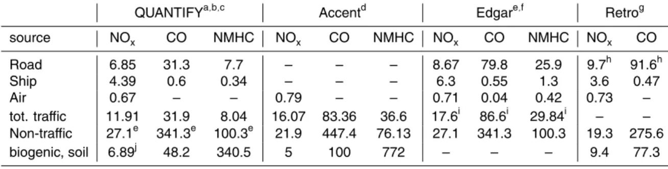
integrated annual emissions which were used in this study for selected species are given in Table 1.

The emissions for ship traffic were reconstructed for QUANTIFY based on fuel- and

activity-based esimates by Endresen et al. (2007). They report a fuel consumption be-ing about 80 Mt lower than in Eyrbe-ing et al. (2005) or Corbett and Koehler (2003). They 20

attribute the difference to the different assumptions for the operation at sea. For further details see Endresen et al. (2007).

Aircraft emissions are based on the AERO2K dataset (Eyers et al., 2004) including the emissions from military aviation. The emissions for each transport sector are given in Table 1.

25

Non-traffic emissions used in the present modelling exercise are based on the latest

(7)

ACPD

8, 18219–18266, 2008

OH

P. Hoor et al.

Title Page

Tables Figures

◭ ◮

Back Close

Full Screen / Esc

Interactive Discussion year 2000 with the exception of methane which was prescribed as a surface boundary

condition.

For biomass burning monthly means for the year 2000 were used based on GFED es-timates with multi-year (1997–2002) averaged activity data using Andreae and Merlet

(2001) and Andreae (2004, personal communication) for NO_x emission factors

(BB-5

AVG-AM). Lightning NOx was specified at 5 TgN/year, representing the current best

estimate (Schumann and Huntrieser, 2007).

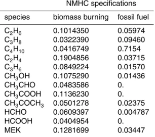
NMHC’s were subdivided into individual organic and partly oxidized species. The par-titioning of the NMHC’s was performed according to von Kuhlmann et al. (2003a) and is shown in Table 2 for biomass burning and fossil fuel related emissions. The mass 10

of NMHC’s given in kg(NMHC)/yr was converted to kg(C)/year using a ratio of 161/210 for molecules(C)/molecules(NMHC). The specific ratios were then applied to calculate the individual NMHC partitioning.

Biogenic emissions for isoprene and NO emissions from soil were also included based on online calculations with the ECHAM5/MESSy model (Ganzeveld et al., 2006; Kerk-15

weg et al., 2006) and provided as offline fields to all partners.

To compare the emissions provided by QUANTIFY with other projects and data bases

some recently used inventories are also given in Table 1. Notably the road traffic

emis-sions are lower than in other inventories. The final road traffic emissions by Borken

et al. (2007) are higher by 33% for NO_x and about 50% for CO emissions than those

20

used in this study. Nonetheless, low total CO emissions are a result of lowered

aver-age emission factors accounting for effective use of catalytic converters in light duty

vehicles.

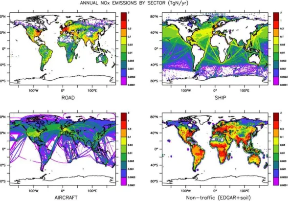
The resulting source strengths of NOx from the different sectors, which were used in

QUANTIFY are shown in Fig. 1. Globally, road NOx emissions are dominated by the

25

(8)

ACPD

8, 18219–18266, 2008

OH

P. Hoor et al.

Title Page

Tables Figures

◭ ◮

Back Close

Full Screen / Esc

source of NO_x over a large area. A second NO_xsource from ship emissions covering

a large area is traffic along the east coast of Asia. Besides the continental eastern US

and western Europe the maximum emissions from air traffic also occur over the North

Atlantic, though further north than the shipping maxima. In the Southern Hemisphere

NOxemissions are largely dominated by non-traffic sources and biomass burning.

5

The simulation period covers the years 2002 and 2003 with 2002 as spin-up. Each participating model calculated the chemical state of the atmosphere for present day conditions using all emissions as described above. The perturbation simulations were performed by reducing the emission of each individual transport sector by 5% (see Table 3). This relatively small reduction was applied to avoid nonlinear responses of 10

the chemical system which would occur by setting the respective emissions to zero. To check for linearity a final simulation was carried out with all transport sectors simul-taneously reduced by 5%. Post processing confirmed the linearity of the small scale

perturbation approach allowing to integrate the e_ffects of the individual transport

sec-tors in this setup. 15

In the following all perturbations are scaled to 100 % unless explicitly mentioned oth-erwise.

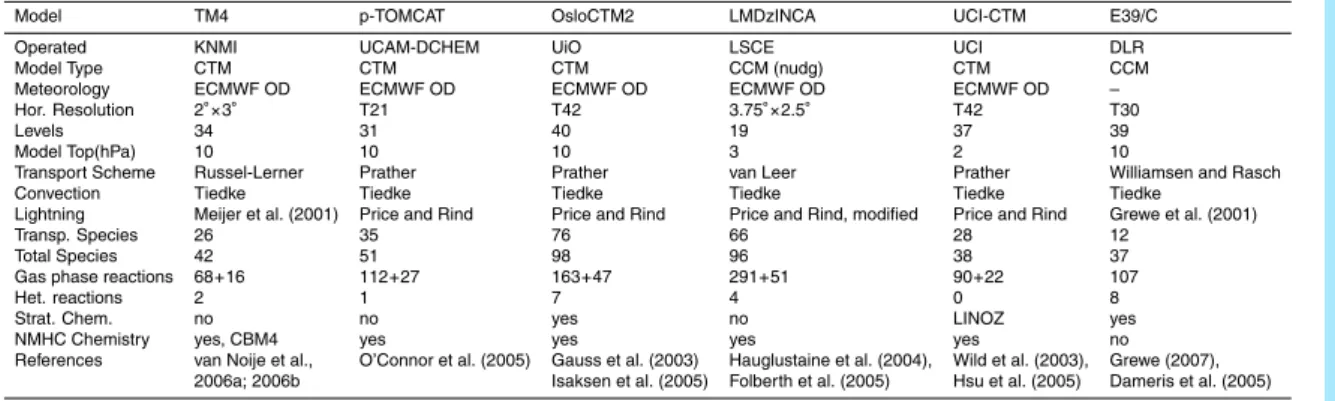
3 Participating models

Six models were applied to estimate the effect of traffic emissions on the current

atmo-spheric chemical composition. Five of them simulated a two years period and included 20

higher order chemistry schemes. One model (E39/C) was used in a different mode to

provide information on the interannual variability of the traffic impact using a ten year

transient simulation. Four models are CTMs using prescribed operational ECMWF data to simulate the meteorological conditions (TM4, p-TOMCAT, OsloCTM2 and UCI). The other two models are coupled CCMs (chemistry climate models). LMDzINCA was 25

(9)

ACPD

8, 18219–18266, 2008

OH

P. Hoor et al.

Title Page

Tables Figures

◭ ◮

Back Close

Full Screen / Esc

Interactive Discussion all models included explicit NMHC chemistry. The TM4 uses a Carbon Bond

Mecha-nism reaction scheme (CBM4) not including acetone chemistry. Three of the models do not include stratospheric chemistry reactions (TM4, p-TOMCAT, LMDzINCA). The number of species ranged from 42(TM4) to 125(LMDzINCA). LMDzINCA and TM4 used their own biogenic and oceanic emissions, respectively (see below).

5

3.1 TM4

The KNMI chemistry transport model TM4 (van Noije et al., 2006a,b) is driven by ECMWF analysed meteorology and contains a chemistry scheme derived from the Carbon Bond Mechanism reaction scheme (CBM4) (Houweling et al., 1998). It was run at a horizontal resolution of 2×3 degrees with 34 model levels from the surface up 10

to 10 hPa.

The lightning parameterisation (Meijer et al., 2001) uses convective precipitation from ECMWF to describe the horizontal distribution of lightning and normalised profiles

cal-culated by Pickering et al. (1998) to distribute lightning produced NO_x vertically

be-tween cloud base and cloud top. 15

Vertical emission profiles were also adopted as included in the respective emission files. In addition to the QUANTIFY emissions oceanic emissions were taken from the

POET emission inventory, ammonia emissions from EDGAR 2.0, and volcanic SO₂

and DMS (Dimethylsulfide) emissions from the standard model configuration of TM4.

3.2 LMDzINCA

20

The CNRS-LSCE model, LMDz-INCA had a resolution of 3.75◦ _{in longitude and 2.5}◦

in latitude with 19 levels extending from the surface up to about 3 hPa and is driven by ECMWF operational data (Hauglustaine et al., 2004).

The NMHC setup of the LMDz-INCA model was used. It considers detailed tropo-spheric chemistry with a comprehensive representation of the photochemistry of non-25

(10)

ACPD

8, 18219–18266, 2008

OH

P. Hoor et al.

Title Page

Tables Figures

◭ ◮

Back Close

Full Screen / Esc

Interactive Discussion anthropogenic, and biomass burning sources.

Most anthropogenic emissions were taken from the EDGAR3.2FT2000 database. The

effective injection height of biomass burning emissions into the atmosphere was taken

into account with the emission heights calculated in the RETRO (REanalysis of the TROpospheric chemical composition over the past 40 years) project. The lightning 5

source was determined interactively in LMDz-INCA with a modified Price and Rind

(1992) parameterization, and its total was prescribed at ≈2. Tg[N]/year. Biogenic

sources were calculated with the vegetation model ORCHIDEE. Oceanic emissions were taken from Folberth et al. (2005).

3.3 OsloCTM2

10

The Oslo CTM2 model is a 3-D chemical transport model driven by ECMWF mete-orological data and extending from the ground to 10 hPa in 40 vertical layers. The

horizontal resolution for this study was Gaussian T42 (2.8◦_×2.8◦_{). The model was}

spun up for several years with emissions from the POET and RETRO projects, then for additional 6 months with the emissions provided for the QUANTIFY project. One 15

restart file was archived for March 2002. From this file the five different scenarios were

started, which were run for 22 months.

3.4 p-TOMCAT

The model used during the first part of the QUANTIFY project is the global offline

chem-istry transport model p-TOMCAT. It is an updated version (see O’Connor et al. (2005)) 20

of a model previously used for a range of tropospheric chemistry studies (Savage et al., 2004; Law et al., 2000, 1998). Convective transport was based on the mass flux pa-rameterization of Tiedtke (1989). The parametrizations includes descriptions of deep and shallow convection with convective updrafts and largescale subsidence, as well as turbulent and organized entrainment and detrainment. The model contains a nonlocal 25

(11)

ACPD

8, 18219–18266, 2008

OH

P. Hoor et al.

Title Page

Tables Figures

◭ ◮

Back Close

Full Screen / Esc

In this study p-TOMCAT was run with a 5.7◦

×5.7◦ horizontal resolution and 31 vertical

levels from the surface to 10 hPa. The offline meteorological fields used are from the

operational analyses of the European Medium Range Weather Forecast model. The chemical mechanism includes the reactions of methane, ethane and propane plus their oxidation products and of sulphur species, it includes 96 bimolecular, 16 termolecular, 5

27 photolysis reactions and 1 heterogeneous reaction on sulphuric acid aerosol. The model chemistry uses the atmospheric chemistry integration package ASAD (Carver et al., 1997) and is integrated with the IMPACT scheme of Carver and Scott (2000). The ozone and nitrogen oxide concentrations at the top model level are constrained to zonal mean values calculated by the Cambridge 2-D model (Law and Nisbet, 1996). 10

The chemical rate coefficients used by p-TOMCAT have been recently updated to those

in the IUPAC Summary of March 2005. The model parameterizations of wet and dry deposition are described in Giannakopoulos et al. (1999).

3.5 UCI

The UCI CTM is a 3-D eulerian chemistry-transport model driven by meteorological 15

data from the ECMWF IFS version cycle 29r2 at T42L40 (see OsloCTM2). Tropo-spheric chemistry is handled by ASAD software package (Carver et al., 1997), con-taining 38 species (28 transported) and 112 reactions (Wild et al., 2003), while in the stratosphere, it employs the stratospheric linear ozone scheme (Linoz) and conducts linear calculations of (P-L) (Hsu, 2004). Photolysis rates are calculated by the Fast-JX 20

package (Bian and Prather, 2002). Transport scheme uses the second order moments (Prather, 1986). Lightning is parameterized with the method of Price and Rind (1992). Convection is simulated, following the ECMWF Tiedtke convection diagnostics.

3.6 E39/C

Impacts by road and ship traffic were provided by DLR based on simulations with

25

(12)

ACPD

8, 18219–18266, 2008

OH

P. Hoor et al.

Title Page

Tables Figures

◭ ◮

Back Close

Full Screen / Esc

Interactive Discussion simulation from 1990 to 1999 (Dameris et al., 2005; Grewe, 2007). The meteorology

is calculated by the climate model ECHAM4.L39(DLR) and therefore does not repre-sent an individual year. Nevertheless, it reprerepre-sents the late 20 century climate and is therefore to some extent comparable to the other simulations of the year 2003. In

particular the emissions which were used by the other participating CTMs are different.

5

The impacts are derived using tagging methods (Grewe, 2004) and hence differ from

the 5% change approach used by other modelling groups in QUANTIFY. However, both methods try to identify the individual contributions from sectors. Changes in the contri-butions are detected comparably by both approaches (Grewe, 2004), i.e. the standard deviation based on interannual variability is similar for both approaches.

10

4 Traffic induced ozone changes

4.1 Total ozone perturbation

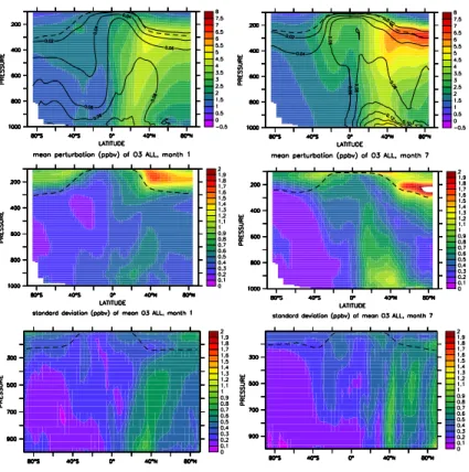
The integrated effect of the emission reduction (ALL-case) by 5% is shown in Fig. 2 for

January and July, respectively. The column ozone distribution change was integrated

from the surface up to 50 hPa. The results from E39/C are not included in the

15

calculation of the mean fields since the results of E39/C were obtained with a different

setup and a different method.

The mean total ozone perturbations in Fig. 2 exhibit strong hemispheric differences of

the traffic emissions with almost zero effect in the Southern Hemisphere, but maximum

effects of about 4 DU during Northern Hemisphere summer (3 DU during winter). All

20

models simulate a similar location of the strongest ozone perturbation extending from the northern subtropical Atlantic to central Europe.

The maximum ozone perturbation is strongest pronounced during northern summer. Interestingly its southern hemispheric seasonal cycle – despite being weak – is in

phase with the Northern Hemisphere with a maximum e_ffect of less than 2 DU. This is

25

(13)

ACPD

8, 18219–18266, 2008

OH

P. Hoor et al.

Title Page

Tables Figures

◭ ◮

Back Close

Full Screen / Esc

occuring during northern summer, which exceed the effects of emissions on the

Southern Hemisphere (see also Fig. 5).

Note furthermore that the effects of traffic emissions over the Pacific and Indian Ocean

downwind of the densly populated coastal areas and sources of pollution, are not

as strong as over the central Atlantic Ocean. A comparison with the NO_x emissions

5

(Fig. 1) indicates that over the northern hemispheric Atlantic in particular ship traffic

and also aircraft emit large amounts of NOx and that these high emissions occur

over a relatively large area. Over the eastern US and western Europe the sum of all three emission categories reach a maximum. Their combination is responsible for the relatively strong perturbations in these regions.

10

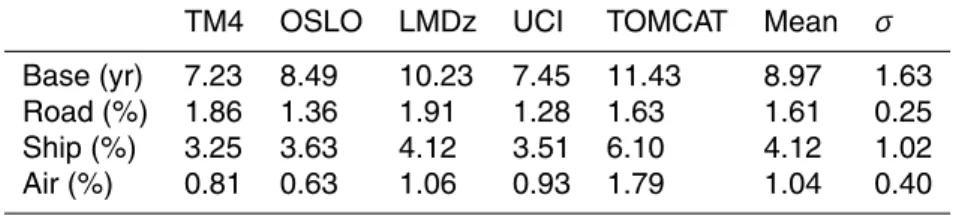
To assess the robustness of the perturbation signal two tests are performed. First

the model to model differences in terms of the associated standard deviation is

assessed to estimate the impact of model uncertainties. Second, the impact of the chosen meteorology (year 2003) is tested by comparing to the interannual variability of the transport signal derived from the transient E39/C simulation, which includes 15

natural variability of the troposphere and the stratosphere due to variations of ozone influx, transport patterns (e.g. induced by El Nino), and others (Grewe, 2007). The

inter-model standard deviations (one-σ) are shown in Fig. 2 (middle). Overall the

models calculate very similar patterns with a relative standard deviation mostly below

15% over large regions of the globe where the effect of the perturbation is strongest.

20

In the Southern Hemisphere, the relative standard deviations are in general somewhat higher (between 20–30%), since the absolute column perturbations are not as large as in the Northern Hemisphere. Largest deviations occur over the tropical central pacific, where concentrations of ozone are still relatively low. Thus, small perturbations may lead to relatively large variations between the models. Note however, that calculated 25

ozone perturbations in particular over Europe and the central Atlantic are relatively robust indicating a significant impact of traffic emissions in these regions.

(14)

ACPD

8, 18219–18266, 2008

OH

P. Hoor et al.

Title Page

Tables Figures

◭ ◮

Back Close

Full Screen / Esc

(bottom) the traffic induced perturbation signal simulated by E39/C over the ten years

period is on the order of 0.8 DU and 1.2 DU in January and July, respectively. Largest variations occur in coastal regions, where synoptic variability leads to advection of either relatively clean maritime air or air from polluted urban areas. Although the perturbation signal from E39/C is largest compared to the other models, the ensemble 5

mean response of the models is still larger than the interannual variability of the transport induced ozone changes according to E39/C. Thus, focusing on a particular year is justified within a 10% uncertainty for ozone since this is the climatological variability simulated consistently within one model.

10

4.2 Zonal mean ozone perturbation

The zonal mean ozone perturbation for the integrated traffic emissions (Fig. 3) shows

the largest effect in the northern subtropics/lower-middle latitudes. In the Northern

Hemisphere boundary layer the mean ozone perturbation peaks at 5.5 ppbv in mid

latitudes at 40–50◦_{N during summer decreasing to less than 3 ppbv during winter.}

15

The perturbation mixing ratio peaks in the upper troposphere/lower stratosphere of the northern extratropics during summer, largely due to aircraft emissions as will be seen later (Fig. 4).

The relative perturbation in the upper troposphere is of the order of 4–6% during

January and July. However, as indicated in Fig. 3 the strongest relative effect can be

20

as large as 16% in the Northern Hemisphere boundary layer during summer. During winter the perturbation peaks at 10% and is located in the tropical boundary layer.

For the Southern Hemisphere the models calculate the strongest absolute effect on

the ozone mixing ratio also for the upper troposphere, although the changes relative to the unperturbed case maximize in the marine boundary layer. In the Southern 25

Hemisphere, both, absolute and relative changes are about 50% lower than in the

Northern Hemisphere. The e_ffect on ozone in the southern boundary layer is only

(15)

ACPD

8, 18219–18266, 2008

OH

P. Hoor et al.

Title Page

Tables Figures

◭ ◮

Back Close

Full Screen / Esc

Interactive Discussion As illustrated in Fig. 3 largest uncertainties between the models are found near the

tropopause and during summer when convection plays an important role in vertical

transport in particular in the northern extratropics. Large emissions by traffic take

place in that latitude belt and thus have the highest probability to be redistributed from the surface to higher altitudes via convection during the summer months. The 5

associated variations between the individual models in that region range from 3.5 ppbv (LMDzINCA) to 6 ppbv (p-TOMCAT) at 250 hPa during July resulting in a standard

deviation of 2 ppbv. In the extratropics of the Southern Hemisphere the e_ffect of

summer convection is not as pronounced due to the hemispheric differences of the

emissions. 10

Interestingly, the interannual variability of the zonal mean ozone perturbations of around 0.5 ppbv (≈5%) for both January and July, is much smaller than the variability among the models (≈20%). This indicates that year-to-year changes in meteorology lead to changes in the horizontal pattern of ozone perturbations (and e.g. convection),

but that the effect of vertical transport and mixing differs less, although horizontally

15

displaced.

4.3 Effects by transport modes

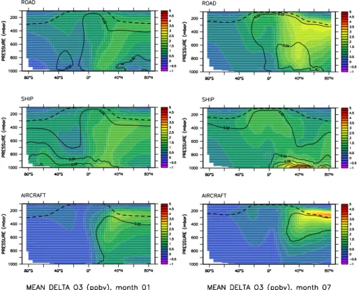
The effects of the respective emissions from road, ship and aircraft on ozone are shown

in Figs. 4–5 for January and July, respectively. The results indicate that the road emis-20

sions have the strongest e_ffect on ozone in the summer boundary layer over the

east-ern US and central Europe extending over the Mediterranean to the Arabian Peninsula (Fig. 4). During winter the average effect of road traffic on ozone in the highly industrial-ized regions of the extratropics almost vanishes or is even inverted. Often under stable boundary layer conditions the emissions accumulate, on average to more than 2 ppbv 25

over the industrialized centers over the eastern US, Europe and parts of East Asia (not

shown). Under these conditions additional NO_x from (road) traffic locally leads to the

(16)

re-ACPD

8, 18219–18266, 2008

OH

P. Hoor et al.

Title Page

Tables Figures

◭ ◮

Back Close

Full Screen / Esc

duced NO_xemissions under high NO_xconditions leading to a higher ozone productivity

per emitted NOx.

Matthes et al. (2007) and Niemeier et al. (2006) find larger relative ozone perturbations

due to road traffic of about 10% for some regions in the Northern Hemisphere

bound-ary layer performing similar model simulations. Part of the deviations to our results can 5

be explained by the use of different emissions, which are based on the EDGAR 1990

fuel estimates in Matthes et al. (2007) and are about 25% higher for NO_x from road

than in this study. The inverted sensitivity of ozone to road emissions during winter is

also reported by Niemeier et al. (2006) with the maximum effect over Europe exceeding

25% at the surface. The latter effect is simulated by all five models in our study, which

10

contribute to the average shown in Fig. 4. Quantitatively, the results of Niemeier et al. (2006) also exceed our calculations by a factor of 2–3 at the surface.

Ship emissions have a significant impact throughout the year also with a maximum in July over the central Atlantic/western European region. In the Northern Hemisphere

their effect dominates the boundary layer perturbation during January and July. Over

15

the northern Pacific region mainly the emission from ships contributes significantly to

the ozone perturbation, whereas the North Atlantic region additionally is a_ffected by

road emissions, which are transported efficiently from the highly polluted Eastern US

to the Atlantic.

Not too surprising, in the northern UTLS region the e_ffect of aircraft emissions

domi-20

nates the ozone perturbation (Fig. 5) being approximately half as large during January compared to July associated with the enhanced level of photochemistry. The ozone

perturbation from road tra_ffic during summer is even higher than the perturbation due

to aircraft emissions in winter, highlighting the role of road traffic for the chemical state of the UTLS in summer (see also Fig. 6). Ship emissions, despite of the high impor-25

tance in the July boundary layer (Fig. 4) do not show a similar e_ffect in the UTLS,

indicating that convective and large scale transport from the marine boundary layer do

not have the same impact as continental convection for road traffic.

(17)

per-ACPD

8, 18219–18266, 2008

OH

P. Hoor et al.

Title Page

Tables Figures

◭ ◮

Back Close

Full Screen / Esc

turbations for the different modes of transportation. Comparing ship and road induced

ozone perturbations ship emissions have a larger impact on boundary layer ozone than

road traffic over the whole year. In the upper troposphere and lower stratosphere the

ozone perturbation from road traffic peaks in summer over in the northern mid

lati-tudes exceeding the effect on the boundary layer. The effect of ship emissions does

5

not exhibit this strong seasonal signal in the upper troposphere although their effect on

surface ozone shows a similar zonal and temporal distribution as for road. Globally the

effect of ship emissions on ozone in the boundary layer larger than those from road

emissions, whereas both are almost equal in the upper troposphere (Table 5). Notably in the upper troposphere aircraft emissions do not dominate the annual mean global 10

e_ffect between 200–300 hPa. Their influence is rather concentrated to latitudes>40◦_N (see. Fig. 5) whereas road and ship traffic affect the UT globally.

These findings are also evident in the vertical zonal mean cross sections (Fig. 5),

high-lighting the importance of surface emissions from ship and road tra_ffic for the tropical

upper troposphere. It also shows that the impact of road traffic is of larger importance

15

for the extratropical troposphere in the northern summer hemisphere. In the tropics ship emissions are the strongest contributor to the ozone perturbation in the tropical transition layer (TTL), being of greater importance than aircraft emissions there. As ev-ident from Fig. 5 the impact of road and ship emissions seems to influence the whole

TTL region from 20◦_S–20◦_{N in particular during northern summer. During January,}

20

when the Inter Tropical Convergence Zone (ITCZ) is located in the Southern

Hemi-sphere, where the emissions are much lower, the TTL is only weakly affected. Note

also that for the upper troposphere in the Southern Hemisphere the e_ffect of ship

emis-sions is among all modes of transport the strongest contributor in January as well as in July (comp. also Fig. 6).

25

4.4 Relative importance of traffic sectors

In addition to the perturbation of O₃ the contribution of the di_fferent transport sectors

(18)

im-ACPD

8, 18219–18266, 2008

OH

P. Hoor et al.

Title Page

Tables Figures

◭ ◮

Back Close

Full Screen / Esc

pact of road and ship emissions differ substantialy although both are released at the

surface. In the region between the surface and 900 hPa the relative e_ffect of ship

emis-sions clearly dominates the total perturbations by all traffic emissions in each summer

hemisphere. In the Southern Hemisphere during January the perturbations of ship emissions can almost contribute up to 85% of the total ozone perturbation, since ship 5

emissions are the major source of pollutants south of 40◦_{S. In the northern}

extratrop-ics the effects from ships are most important in the boundary layer below 950 hPa,

where the mean perturbation relative to the background can be as high as 16% (see also Fig. 7). As evident from Fig. 7 the contribution of ship emissions is particularly important in the subtropical monsoon regions and the tropics, where convection leads 10

to upward transport of the emissions and to a relative contribution of 50% up to the tropical tropopause.

The relative contribution of road emissions peaks in the free troposphere in both summer hemispheres with a pronounced seasonal cycle in the northern extratropics.

The maximum effect on ozone occurs in July, when convection at these latitudes is

15

strongest. Thus during that time of the year pollutants from road traffic have a much

higher probability to be transported to tropopause altitudes compared to winter. This is also evident from Fig. 5 where the ozone perturbations in July below the tropopause are almost equal to the effect from aircraft.

Note that ship emissions do only weakly affect the free and upper troposphere of the

20

northern extratropics during July. Since ships largely emit over the open oceans where convection is not as strong as over the continents, they have a much lower potential to reach the upper troposphere of the extratropics compared to road emissions. There-fore, in the winter hemispheres the effects of road and ship traffic on ozone show similar

patterns (Fig. 5). As indicated by Fig. 7 the relative contribution of road traffic on the

25

(19)

ACPD

8, 18219–18266, 2008

OH

P. Hoor et al.

Title Page

Tables Figures

◭ ◮

Back Close

Full Screen / Esc

To estimate the efficiency of the ozone perturbation from each transport sector we

normalized the ozone perturbation of each sector to the respective number of NO_x

molecules assuming a global average lifetime of 22 days for ozone (Stevenson et al.,

2006). As evident from Table 6 road and ship emissions have similar efficiencies to

perturb ozone. However, the NO_x emissions from air tra_ffic are more than twice as

5

efficient in producing ozone. Since these emissions take place in the UTLS region the

lifetime of the reservoir species HNO3 and PAN are much longer than at the surface.

Therefore each NO_x molecule can be recycled more often to produce ozone before

being removed via precipitation scavenging and dry deposition of HNO3.

Note that despite some individual differences, all models indicate the largest efficiency 10

to perturb ozone for NO_x emissions from aircraft and the weakest e_fficiency for road

traffic.

5 OH

5.1 Global OH

The effects of different transport systems on tropopspheric OH concentrations are

15

shown in Fig. 8 for January and July, respectively. Interestingly, ship emissions have the largest impact on the global OH budget in the boundary layer. During northern summer

the effect of NOxfrom maritime traffic on OH can be as large as 5·10

5

molecules/cm3

at 40◦_{N equivalent to an increase of up to 15%. During winter the e}

ffect of ship emis-sions is about a factor of two lower, thereby reaching a maximum in the latitude band 20

from 40◦_{S to 30}◦_{N. Since the OH concentrations are globally highest in these regions,}

the increase by about 5·105molecules/cm3is of similar magnitude as the annual mean

concentration in temperate and high latitudes, and is therefore highly significant on a global scale. Also in winter the boundary layer OH perturbation is still of the order of 10%. As can be seen from Fig. 8 ship emissions are dominating the annual zonal 25

(20)

ACPD

8, 18219–18266, 2008

OH

P. Hoor et al.

Title Page

Tables Figures

◭ ◮

Back Close

Full Screen / Esc

The effect of road emissions on the OH distribution shows a pronounced seasonal

cycle in particular in the Northern Hemisphere. The maximum effect occurs during

northern summer in the continental boundary layer between 800–900 hPa reaching

1·105 molecules/cm3 or about 3.5% (zonal annual mean). Since road emissions are

largely emitted at some elevation over the continents the zonal mean effect on OH

5

at 1000 hPa is less pronounced compared to 900 hPa. However, in particular during northern summer road transport seems to be most important for the lower troposphere in the extratropics up to 500 hPa.

The horizontal distribution (Fig. 9) reveals that the effect on a regional basis can

be much stronger than 1·105 molecules/cm3. The largest impact is found in the

10

industrialized regions of the Eastern US, central Europe and East Asia reaching

5·105 molecules/cm3. In these regions OH has the highest potential to be recycled

via the reaction of NO with HO2, which is produced after the initial reaction of OH on

the carbon containing reactive species (e.g. CO, CH₄, NMHCs). The additional NO₂

from this reaction in turn leads to the enhanced formation of ozone and OH production 15

via O1(D). During winter the emissions of CO and NMHCs in these regions act as a

direct sink, since solar radiation is reduced.

Comparing the impact of road and ship traffic, both surface sources of air pollution, the

effects on OH are very different, although the annual amount of emitted NOxis similar

(see Table 1). The zonal mean perturbation of road peaks at about 4% during north-20

ern summer and 2% in the Southern Hemisphere summer. The regional effect during

July can exceed 10% in the continental boundary layer for road traffic. As evident from

Fig. 8 ship emissions have a larger e_ffect even in the zonal mean. The large di_fferences

of both means of transportation on OH can be related to the different regions and

pol-lution conditions. As will be seen later, the sensitivity of OH to traffic emissions is

25

largest in the still relatively pristine regions over the (sub-)tropical oceans. Background

concentrations of ozone, NOx and other NMHCs are low, and the solar irradiation and

water vapor available for OH formation are high. The recycling potential of OH by NOx

(21)

ACPD

8, 18219–18266, 2008

OH

P. Hoor et al.

Title Page

Tables Figures

◭ ◮

Back Close

Full Screen / Esc

reason is that at already enhanced NO_x levels the reaction of OH with NO₂ becomes

a significant sink of hydroxyl radicals, which is not the case in the NOx-poor marine

boundary layer. On the other hand these low NOx concentrations accompanied with

high OH make the system more sensitive for NO_xperturbations than in polluted areas

(Lelieveld et al., 2002). Furthermore, road emissions occur at higher altitudes and lati-5

tudes where average water vapor concentrations and solar irradiation are lower and in

regions where other anthropogenic sources of pollution cause enhanced NO_x levels.

The combination of these factors leads to a lower sensitivity of OH to perturbations from road traffic than for ship emissions.

The regional perturbation pattern (Fig. 9) illustrates that locally the effects of road and 10

ship emissions on OH are similar during northern summer. The strongest e_ffect is

sim-ulated for the ship emissions over the northern subtropical Atlantic in the same region where also ozone exhibits the largest perturbation (see Fig. 4). Note furthermore that

in particular during northern summer the e_ffect on OH at high northern latitudes over

Europe is as high as over the eastern subtropical Pacific. Thus the increasing ship 15

traffic at high northern latitudes as a response to the diminishing ice coverage due to

the relatively rapid climate change (Lemke et al., 2007, IPCC) might have strong e_ffects

on the oxidation capacity and therefore on the composition of the atmosphere in high latitudes.

Similar to ozone, aircraft emissions have the largest e_ffect on OH in the upper

tropo-20

sphere of the northern extratropics during summer. Despite the fact that the absolute perturbation is about a factor of 2 lower during winter, the relative perturbation exceeds 12%. The larger relative change during northern winter is due to the strong seasonal variation of the background latitudinal OH distribution. During winter the extratropical

zonal mean OH at 300 hPa is less than 1·105molecules/cm3, whereas in summer the

25

mean OH in the same region is reaching 2.5·105molecules/cm3.

(22)

ACPD

8, 18219–18266, 2008

OH

P. Hoor et al.

Title Page

Tables Figures

◭ ◮

Back Close

Full Screen / Esc

Interactive Discussion favourable for OH production than further north. Notice that ship emissions also

sig-nificantly contribute to the OH perturbation in the middle to upper troposphere of the

subtropics up to 200 hPa caused by convective uplift of NOxfrom maritime transport in

the tropical and subtropical latitudes.

5.2 Methane lifetime

5

As seen in the previous section ship emissions have the largest effect on OH leading

to the largest reduction of methane lifetime (Table 7) among the three major modes of

transport. Road emissions are only half as efficient in perturbing OH on a global scale,

and the effects of air traffic are the smallest. The changes by 4.12% (ensemble mean)

due to ship emissions exceed the 1.56% reported by Eyring et al. (2007), although 10

their emissions of 3.1 TgN/yr are not very much lower compared to the 4.4 TgN/yr in this study (see Table 1). However, the distribution of the ship emissions in Eyring et al. (2007) and Stevenson et al. (2006) is based on the EDGAR3.2 dataset, where the emissions are mainly concentrated on the major shipping routes. The ship emissions used in QUANTIFY have been generated by merging the daily fields of COADS and 15

AMVER data (Automated Mutual-assistance Vessel Rescue system) (Endresen et al., 2003) and are distributed over a larger area (comp. Fig. 1 and Eyring et al. (2007), their Fig. 1). This explains the stronger e_ffect on CH₄lifetime, since a larger fraction of NO_x is emitted over the tropical oceans over a widespread area. Recall that conditions for

OH production are favourable at low latitudes and in addition the local CH4lifetime by

20

OH oxidation is shortest also due to the high temperatures.

Both factors are also the reason for the smaller effects of road and aircraft emissions

(23)

ACPD

8, 18219–18266, 2008

OH

P. Hoor et al.

Title Page

Tables Figures

◭ ◮

Back Close

Full Screen / Esc

5.3 Sensitivity of OH production

From Fig. 9 it is evident that ship emissions strongly affect the still relatively clean re-gions mostly in the tropics, but also in the extratropics. In contrast, road emissions are

largely released into an environment already affected by emissions from other sources

both of natural (soils, lightning) and anthropogenic origin. The different effects on OH

5

from road and ship traffic in the boundary layer are presented in Fig. 10 showing the

∆NOxand∆OH perturbations for road and ship emissions, respectively. Coloured data

points are indicative for low NOx conditions (<20 pptv) in different latitude belts. The

correlations show that the sensitivity of OH to NO_xperturbations is much higher for ship

traffic than for road emissions even under low-NOxconditions. As expected the∆OH/∆

10

NOx-ratio is highest for ship emissions in the relatively pristine maritime conditions in

the tropics (red). The impact of road emissions is insignificant in these regions under

low-NOx conditions. In particular in the southern extratropics (green dots) there is a

high sensitivity to NOxperturbations from ships.

In relatively NOx enriched conditions, under which most of the road emissions occur,

15

the e_ffect of ship NO_x on OH is also higher than that of road tra_ffic. The OH response

for ship emissions is an almost linear function at the lower∆NOx levels, whereas the

efficiency of OH production from road is weaker and levels offat lower∆NOx

pertur-bations. OH perturbations from road NO_xemissions maximize at 4·105molecules/cm3,

while OH perturbations from ship exceed 5·105molecules/cm3 and show no

satura-20

tion tendency. This can be attributed to the higher level of NMHCs and NO2 over the

continents acting as a sink for OH at high pollution levels.

6 Conclusions

In the frame of QUANTIFY the combined and relative effects of road, ship and aircraft

emissions on the composition of the current atmosphere has been investigated. Six 25

(24)

ACPD

8, 18219–18266, 2008

OH

P. Hoor et al.

Title Page

Tables Figures

◭ ◮

Back Close

Full Screen / Esc

Interactive Discussion small (5%) perturbation approach. The results especially highlight the global impact

of ship emissions on the chemical state of the marine boundary layer. Directly at the surface their impact can exceed 10% relative to the ozone backround contributing 60–

80% to the total perturbation by traffic. They strongly contribute to the tropospheric

ozone column perturbation of 4 DU over the Atlantic Ocean. 5

For the global OH budget the effect of ship emissions is most important accounting for

a perturbation up to 5·105molecules/cm3equivalent to about 15% relative to the base

case. Since emissions of NO_x largely occur in the pristine regions in the (sub-)tropics

they efficiently lead to OH-formation and to additional ozone production. The

conse-quent reduction of the lifetime of methane is about 4% for ship traffic while road and

10

aircraft lead to 1.8% and 1% changes, respectively.

Road emissions in the Northern Hemisphere affect ozone in particular during summer,

when the low solar zenith angles in the extratropics enhance photochemistry. Conti-nental convection leads to vertical redistribution of the road emissions resulting in a significant contribution to the ozone perturbation in the northern extratropical UTLS of 15

3.5 ppbv being about 30% of the aircraft effect on ozone at 250–300 hPa. The efficiency

of ozone production per NO_xmolecule emitted is highest for aircraft emissions (22 O₃

-molecules/molecule NOx), whereas the efficiencies for ozone from ship or road NOx

are around 10 and 6 O3-molecules/molecule NOx, respectively. The high efficiency of

air traffic on ozone perturbations arises from the relatively long lifetime of NO_x and its 20

reservoir species PAN and HNO3at the altitudes where the emissions occur.

Acknowledgements. The QUANTIFY project is funded by the European Union within the 6th research framework programmme under contract 003893.

25

(25)

ACPD

8, 18219–18266, 2008

OH

P. Hoor et al.

Title Page

Tables Figures

◭ ◮

Back Close

Full Screen / Esc

References

Andreae, M. and Merlet, P.: Emission of trace gases and aerosols from biomass burning, Global Biogeochem. Cy., 15, 955–966, 2001. 18225

Bian, H. and Prather, M.: Fast-J2: Accurate Simulation of stratospheric photolysis in global chemical models, J. Atmos. Sci., 41, 281–296, 2002. 18229

5

Borken, J. and Steller, H.: Report on the Draft Emission Inventories for Road Transport in the year 2000, Tech. rep., Deutsches Institut f ¨ur Luft- und Raumfahrt (DLR), Institut f ¨ur Verkehrs-forschung, 2006. 18224

Borken, J., Steller, H., Meretei, T., and Vanhove, F.: Global and country inventory of road passenger and freight transportation - Their fuel consumption and their emissions of air 10

pollutants in the year 2000, Transportation Research Records, Journal of the Transportation Research Board, 2011, doi:10.3141/2011-14, 127–136, 2007. 18224, 18225

Brasseur, G. P., M ¨uller, J., and Garnier, C.: Atmospheric impact of NO_xemissions by subsonic aircraft: A three-dimensional model study, J. Geophys. Res., 101, 1423–1428, 1996. 18222 Carver, G. and Scott, P.: IMPACT: an implicit time integration scheme for chemical species and 15

families, Ann. Geophys., 18, 337–346, 2000, http://www.ann-geophys.net/18/337/2000/. 18229

Carver, G., Brown, P., and Wild, O.: The ASAD atmospheric chemistry integration package and chemical reaction database, Comp. Physics Communications, 105, 197–215, 1997. 18229 Corbett, J. and Koehler, H.: Updated emissions from ocean shipping, J. Geophys. Res., 108, 20

4650, doi:10.1029/2003JD003751, 2003. 18222, 18224

Dalsoren, S. and Isaksen, I.: CTM study of changes in tropospheric hydroxyl distribution 1990–2001 and its impact on methane, Geophys. Res. Lett., 33, L23811, doi:10.1029/ 2006GL027295, 2006. 18222, 18223

Dameris, M., Grewe, V., Ponater, M., Deckert, R., Eyring, V., Mager, F., Matthes, S., Schnadt, 25

C., Stenke, A., Steil, B., Br ¨uhl, C., , and Giorgetta, M.: Long-term changes and variability in a transient simulation with a chemistry-climate model employing realistic forcing, Atmos. Chem. Phys., 5, 2121–2145, 2005,

http://www.atmos-chem-phys.net/5/2121/2005/. 18230, 18253

Endresen, O., Sorgand, E., Sundet, J., Dalsoren, S., Isaksen, I., Berglen, T., and Gravir, G.: 30

(26)

ACPD

8, 18219–18266, 2008

OH

P. Hoor et al.

Title Page

Tables Figures

◭ ◮

Back Close

Full Screen / Esc

Interactive Discussion Endresen, O., Sorgard, E., Behrens, H., Brett, P., and Isaksen, I.: A historical

recon-struction of ships’ fuel consumption and emissions, J. Geophys. Res., 112, D12301, doi:10.1029/2006JD007630, 2007. 18222, 18224

Eyers, C., Norman, P., Middel, J., Plohr, M., Michot, S., Atkinson, K., and Christou, R.: AERO2K Global Aviation Emissions Inventories for 2002 and 2025, Tech. Rep. 04/01113, QinetiQ, 5

http://elib.dlr.de/1328, 2004. 18224

Eyring, V., K ¨ohler, H., J., v., and Lauer, A.: Emissions from international shipping: 1. The last 50 years, J. Geophys. Res., 110, D17305, doi:10.1029/2004JD005619, 2005. 18222, 18224 Eyring, V., Stevenson, D. S., Lauer, A., Dentener, F. J., Butler, T., Collins, W. J., Ellingsen, K., Gauss, M., Hauglustaine, D. A., Isaksen, I. S. A., Lawrence, M. G., Richter, A., Rodriguez, 10

J. M., Sanderson, M., Strahan, S. E., Sudo, K., Szopa, S., van Noije, T. P. C., and Wild, O.: Multi-model simulations of the impact of international shipping on Atmospheric Chemistry and Climate in 2000 and 2030, Atmos. Chem. Phys., 7, 757–780, 2007,

http://www.atmos-chem-phys.net/7/757/2007/. 18222, 18240

Folberth, G., Hauglustaine, D., Ciais, P., and Lathi ¨are, J.: On the role of atmospheric chemistry 15

in the global CO₂ budget, Geophys. Res. Lett., 32, L08801, doi:10.1029/2004GL021812, 2005. 18228, 18253

Ganzeveld, L., van Aardenne, J., Butler, T., Lawrence, M., Metzger, S., Stier, P., Zimmermann, P., and Lelieveld, J.: Technical Note: Anthropogenic and natural offline emissions and the online EMissions and dry DEPosition submodel EMDEP of the Modular Earth Submodel 20

system (MESSy), Atmos. Chem. Phys. Discuss., 6, 5457–5483, 2006, http://www.atmos-chem-phys-discuss.net/6/5457/2006/. 18225, 18250

Gauss, M., Isaksen, I., Wong, S., and Wang, W.-C.: Impact of H₂O emissions from cryoplanes and kerosene aircraft on the atmosphere, J. Geophys. Res., 108, 4304, doi:doi:10.1029/ 2002JD002623, 2003. 18253

25

Gauss, M., Isaksen, I. S. A., Lee, D. S., and Svde, O. A.: Impact of aircraft NO_x emissions on the atmosphere - tradeoffs to reduce the impact, Atmos. Chem. Phys., 6, 1529–1548, 2006, http://www.atmos-chem-phys.net/6/1529/2006/. 18222

Giannakopoulos, C., Chipperfield, M., Law, K., and Pyle, J.: Validation and intercomparison of wet and dry deposition schemes using 210Pb in a global three-dimensional off-line chemical 30

transport model, J. Geophys. Res., 104, 23 761–23 784, 1999. 18229

(27)

ACPD

8, 18219–18266, 2008

OH

P. Hoor et al.

Title Page

Tables Figures

◭ ◮

Back Close

Full Screen / Esc

Interactive Discussion Grewe, V.: Technical note: A diagnostic for ozone contributions of various NO_x emissions in

multi-decadal chemistry-climate model simulations, Atmos. Chem. Phys., 4, 327–342, 2004, http://www.atmos-chem-phys.net/4/327/2004/. 18230

Grewe, V.: Impact of climate variability on tropospheric ozone, Sci. Tot. Env., 374, 167–181, 2007. 18230, 18231, 18253

5

Grewe, V., Brunner, D., Dameris, M., Grenfell, J., Hein, R., Shindell, D., and Staehelin, J.: Origin and variability of upper tropospheric nitrogen oxides and ozone at northern mid-latitudes, Atmos. Environ., 35, 3421–3433, 2001. 18253

Grewe, V., Dameris, M., Fichter, C., and Sausen, R.: Impact of aircraft NOX emissions. Part I: Interactively coupled climate-chemistry simulations and sensitivities to climate-chemistry 10

feedback, lightning and model resolution, Meteor. Z., 177–186, 2002. 18222

Grewe, V., Stenke, A., Ponater, M., Sausen, R., Pitari, G., Iachetti, D., Rogers, H., Dessens, O., Pyle, J., Isaksen, I., Gulstad, L., Sovde, O., Marizy, C., and Pascuillo, E.: Climate impact of supersonic air tra_ffic: an approach to optimize a potential future supersonic fleet - results from the EU-project SCENIC, Atmos. Chem. Phys., 7, 5129–5145, 2007,

15

http://www.atmos-chem-phys.net/7/5129/2007/. 18222

Hauglustaine, D., Hourdin, F., Walters, S., Jourdain, J., Filiberti, M.-A., Lamarque, J.-F., and Holland, E.: Interactive chemistry in the Laboratoire de Mtorologie Dynamique general cir-culation model: Description and background tropospheric chemistry evaluation, J. Geophys. Res., 109, D04314, doi:10.1029/2003JD003957, 2004. 18227, 18253

20

Hedegaard, G., Brandt, J., Christensen, J. H., Frohn, L. M.and Geels, C., Hansen, K. M., and Stendel, M.: Impacts of climate change on air pollution levels in the Northern Hemisphere with special focus on Europe and the Arctic, Atmos. Chem. Phys., 8, 3337–3367, 2008, http://www.atmos-chem-phys.net/8/3337/2008/. 18222

Hidalgo, H. and Crutzen, P.: The tropospheric and stratospheric composition perturbed by NOx 25

emissions of high-altitude aircraft, J. Geophys. Res., 82, 5833–5866, 1977. 18222

Holtslag, A. A. M. and Boville, B.: Local vesus nonlocal boundary-layer diffusion in a global climate model, J. Climate, 6, 1825–1842, 1993. 18228

Houweling, S., Dentener, F., and Lelieveld, J.: The impact of nonmethane hydrocarbon com-pounds on tropospheric photochemistry, J. Geophys. Res., 103, 10 673–10 696, 1998. 18227 30

(28)

ACPD

8, 18219–18266, 2008

OH

P. Hoor et al.

Title Page

Tables Figures

◭ ◮

Back Close

Full Screen / Esc

Interactive Discussion Hsu, J. e. a.: Are the TRACE-P measurements representative of the western Pacific during

March 2001?, J. Geophys. Res., 109, D02314, doi:10.1029/2003JD004002, 2004. 18229 Isaksen, I., Zerefos, C., Kourtidis, K., Meleti, C., Dalsoren, S., Sundet, J., Grini, A.,

Za-nis, P., and Balis, D.: Tropospheric ozone changes at unpolluted and semipolluted re-gions induced by stratospheric ozone changes, J. Geophys. Res., 110, D02302, doi: 5

10.1029/2004JD004618, 2005. 18253

Kahn Ribeiro, S., Kobayashi, S., Beuthe, M., Gasca, J., Greene, D., Lee, D., Muromachi, Y., Newton, P., Plotkin, S., Sperling, D., Wit, R., and Zhou, P.: Transport and its infrastructure, in: Climate Change 2007: Mitigation. Contribution of Working Group III to the Fourth Assess-ment Report of the IntergovernAssess-mental Panel on Climate Change, IPCC, edited by Metz, B., 10

Davidson, O., Bosch, P., Dave, R., and Meyer, L., Cambridge University Press, Cambridge, United Kingdom and New York, NY, USA, 2007. 18222

Kerkweg, A. and, S. R., Tost, H., and J ¨ockel, P.: Technical note: Implementation of prescribed (OFFLEM), calculated (ONLEM), and pseudo-emissions (TNUDGE) of chemical species in the Modular Earth Submodel System (MESSy), Atmos. Chem. Phys., 6, 3603–3609, 2006, 15

Law, K. and Nisbet, E.: Sensitivity of the methane growth rate to changes in methane emissions from natural gas and coal, J. Geophys. Res., 101, 14 387–14 397, 1996. 18229

Law, K., Plantevin, P., Shallcross, D., Rogers, H., Pyle, J., Grouhel, C., Thouret, V., and Marenco, A.: Evaluation of modelled O₃using MOZAIC data, J. Geophys. Res., 103, 25 721– 20

25 737, 1998. 18228

Law, K., Plantevin, P., Thouret, V., Marenco, A., Asman, W., Lawrence, M., Crutzen, P., Muler, J., Hauglustaine, D., and Kanakidou, M.: Comparison between global chemistry transport model results and Measurement of Ozone and Water Vapor by Airbus In-Service Aircraft (MOZAIC) data, J. Geophys. Res., 105, 1503–1525, 2000. 18228

25

Lawrence, M. G. and Crutzen, P. J.: Influence of NOx emission from ships on tropospheric photochemistry and climate, Nature, 402, 167–170, 1999. 18222

Lelieveld, J., Peters, W., Dentener, F., and Krol, M.: Stability of tropospheric hydroxyl chemistry, J. Geophys. Res., 107, 4715, doi:10.1029/2002JD002272, 2002. 18223, 18239

Lelieveld, J., Dentener, F., Peters, W., and Krol, M.: On the role of hydroxyl radicals in the self-30

cleansing capacity of the troposphere, Atmos. Chem. Phys., 4, 2337–2344, 2004, http://www.atmos-chem-phys.net/4/2337/2004/. 18223

(29)

ACPD

8, 18219–18266, 2008

OH

P. Hoor et al.

Title Page

Tables Figures

◭ ◮

Back Close

Full Screen / Esc

Interactive Discussion Thomas, R., and T., Z.: Observations: Changes in Snow, Ice and Frozen Ground, in: Climate

Change 2007: The Physical Science Basis. Contribution of Working Group I to the Fourth Assessment Report of the Intergovernmental Panel on Climate Change, IPCC, edited by Solomon, S., Qin, D., Manning, M., Chen, Z., Marquis, M., Averyt, K., Tignor, M., and Miller, H., Cambridge University Press, Cambridge, United Kingdom and New York, NY, USA, 2007. 5

18239

Matthes, S., Grewe, V., Sausen, R., and Roelofs, G.: Global impact of road traffic emissions on tropospheric ozone, Atmos. Chem. Phys., 7, 1707–1718, 2007,

http://www.atmos-chem-phys.net/7/1707/2007/. 18222, 18223, 18234

Meijer, E., van Velthoven, P., Brunner, D., Huntrieser, H., and Kelder, H.: Improvement and 10

evaluation for the parametrisation of nitrogen oxide production by lightning, Phys. Chem. of the Earth, 26/8, 557–583, 2001. 18227

Niemeier, U., Granier, C., Kornblueh, L., Walters, S., and Brasseur, G.: Global impact of road tra_ffic on atmospheric chemical composition and on ozone climate forcing, J. Geophys. Res., 111, D09301, doi:10.1029/2006JD006407, 2006. 18222, 18223, 18234

15

O’Connor, F., Carver, G., Savage, N., Pyle, J., Methven, J., Arnold, S., Dewey, K., and Kent, J.: Comparison and visualisation of high-resolution transport modelling with aircraft measure-ments, Atm. Sci. Lett., 6, 164–170, doi:10.1002/asl.111, 2005. 18228, 18253

Ohara, T., Akimoto, H., Kurokawa, J., Horii, N., Yamaji, K., Yan, X., and Hayasaka, T.: An Asian emission inventory of anthropogenic emission sources for the period 1980–2020, Atmos. 20

Chem. Phys., 7, 4419–4444, 2007,

Olivier, J., van Aardenne, J., Dentener, F., Ganzeveld, L., and Peters, J.: Recent trends in global greenhouse gas emissions: regional trends and spatial distribution of key sources, in: Non-CO₂Greenhouse Gases (NCGG-4), pp. 325–330, Millpress, Rotterdam, 2005. 18224 25

Pickering, K. E., Wang, Y., Tao, W., Price, C., and Muller, J.-F.: Vertical distribution of light-ning NOx for use in regional and global chemical transport models, J. Geophys. Res., 109, 31 203–31 216, 1998. 18227

Prather, M.: Numerical advection by conservation of second-order moments, J. Geophys. Res., 91, 6671–6681, 1986. 18229

30

Price, C. and Rind, D.: A simple lightning parameterization for calculating global lightning dis-tributions, J. Geophys. Res., 97, 9919–9933, 1992. 18228, 18229