Infiltration in the Corgo River basin (northern Portugal): coupling water balances with rainfall—runoff regressions on a monthly basis

INFILTRATION IN THE CORGO RIVER BASIN (NORTH OF PORTUGAL): COUPLING WATER

BALANCES WITH RAINFALL-RUNOFF REGRESSIONS ON A MONTHLY BASIS

Ana Maria Pires Alencoão

and Fernando António Leal Pacheco

1

Geology Department, Trás-os-Montes e Alto Douro University, 5000 Vila Real, Portugal

2

Centre for Geophysics, Coimbra University, 3000 Coimbra, Portugal

3

ABSTRACT

A combination of water balances and rainfall-runoff regressions is used to calculate infiltration (I),

overland flow (Qs), base flow (Qg) and change to the surface water reservoir (s), on a monthly

basis; evapotranspiration from the underground reservoir (ET

), on an annual basis; and a lag phase

of maximum I and maximum Qg (tg) within a hydrological year. The water balance equations are

written for catchment areas shaped on crystalline rocks and located in temperate climates. The

regression lines are fitted to precipitations (P) and river flows (Q

). The model is tested with the

Corgo river hydrographic basin, a small watershed in the Trás-os-Montes and Alto Douro province,

north of Portugal. The results are (values in mm y

): I = 345.8, Qs = 444.2, Qg = 303.1, s = 0.5

(steady state), ET

= 42 and t

= 4 months. They compare favourably with results of other groups,

working under similar environmental conditions.

INTRODUCTION

There are numerous ways for estimating the infiltration of meteoric water into the soil and bedrock.

In a recent review, Scanlon et al. (2002) subdivided the available techniques on the basis of three

hydrologic sources (or zones) from which the data are obtained, namely surface water, unsaturated

zone and saturated zone. Further, within each zone the surveyed methods were classified into

physical, tracer or numerical approaches.

The objective of a study plays an important role in determining the appropriate technique for

quantifying infiltration, because the goal determines the space and time scales required. In this

study, the main purpose was to evaluate groundwater resources at the watershed scale and at time

scales of a month to a year, using a method based on easily available data (long-term rainfall, runoff

and temperature records). The secondary objective was to obtain input data for subsequent

weathering studies. In this context, the assessment of infiltration (or base flow) is vital for the

estimation of mineral weathering rates (Pacheco and Van der Weijden, 2002; Van der Weijden and

Pacheco, 2003; Pacheco and Alencoão, 2005).

The methods based on data from the unsaturated and saturated zones are beyond the scope of this

paper, as they are not based on easily available data, and can be found elsewhere (e.g., Belan and

Matlock, 1973; Verhagen, 1992; Hendrickx and Walker, 1997; Scanlon et al., 1997; Gee and Hillel,

1998; Zhang, 1998; Cook et al., 1998, 2001). Among the methods based on surface water data (e.g.,

Lerner, 1997; Ronan et al., 1998; Rosenberry, 2000; Halford and Mayer, 2000), the most adequate

technique for this study is the watershed modeling. Recently, Shaw (1994) as well as Beven (2001)

summarized the latest findings which represent the state of the art on this subject. From the cited

reviews one may distinguish process-oriented models, which conceive the hydrology of a drainage

basin as a series of inter linked processes and storages (Dawdy and O'Donnel, 1965; Jonch-Clausen,

1979), but in general use an awesome number of input variables which may result in increasing

problems of calibration and therefore be a source of uncertainty (Todini, 1996; Flint et al., 2000,

2002; Ciarapica and Todini, 2002), from conceptual water balance models, which are oriented

towards simpler mathematical formalizations and built on a limited number of parameters.(e.g.

Xiong and Guo, 1999).

In this paper, a monthly water balance model is introduced. Relative to comparable algorithms (a

review is provided by Xu and Singh, 1998), the distinctive feature of our method is the coupling of

regression equations between rainfall and river flow with water-balance equations, for solving for

unknown components of the water balance (e.g. infiltration and base flow). Further, infiltration

(input to the underground reservoir) and base flow (output) are determined separately on a monthly

basis, which enables the calculation of a lag phase of maximum infiltration and maximum base

flow. This approach may provide an effective tool to the hydrologist who is seeking for ways of

evaluating groundwater resources in temperate climates. The object of this study is the Corgo river

basin, a small watershed in Trás-os-Montes and Alto Douro, north Portugal.

WATER BALANCES AND RAINFALL-RUNOFF REGRESSIONS

Premises

The method developed in this study estimates components of the water-balance equation by

combining this equation with rainfall-runoff regressions on a monthly basis. The spatial scale is the

watershed scale, the time scales are the monthyear scales. The algorithm is applicable to any

region of temperate climate, with cold-wet and warm-dry seasons. The cold-wet season is a period

of water surplus, i.e. a period with precipitation (P) in excess of potential evapotranspiration (ETP)

that usually goes from autumn to early spring. The warm-dry season has ETP > P and runs from late

spring to summer. In any case, the river basins must be shaped on massifs of crystalline rocks with a

limited coverage by alluvial aquifers. The underground trajectory of precipitation water inside the

basins must start in the top soil, where it can feed evapotranspiration or proceed throughout the

saprolite and rock fractures, ultimately ending up in the river as base flow.

The water balance

Figure 1 depicts the main components of the water balance at the watershed scale. In such system,

the surface (s) and underground (g) water reservoirs are in permanent change. The source of

water to the catchment is rainfall (P), which is partially lost as direct evaporation (E

) or overland

flow (Qs), before entering the underground reservoir as infiltration (I). Part of the infiltrated water

returns to the atmosphere as evapotranspiration (ETm), while the other part emerges as base flow

(Qg), after a period of underground flow, or remains in storage. The net infiltration (R = IETm) is

termed groundwater recharge. The measured river flow, also known as runoff (Qr), accounts for the

surface plus groundwater contributions, to which direct evaporation from the river channel (Er) and

changes to the surface water reservoir (s) may have to be deduced. The water balance model

considered in this study can be summarized by the following equations:

River flow balance: Q

= Q

+ Q

– E

 

(1a)

Overland flow balance: Qs = P – Ep – I

(1b)

Underground reservoir balance: g = I  ETm  Qg

(1c)

It should be noted that Equations 1ac ignore any man's influences, such as abstractions from

groundwater and rivers, or discharges such as sewage and industrial effluents, but in many small

watersheds throughout the world these influences are localized and not comparable to the system's

natural inputs and outputs.

Rainfall-runoff regressions

The derivation of relationships between the rainfall over a catchment area and the resulting flow in

a river is very much dependent on the time scale being considered. For short durations (hours) the

complex interrelationship between rainfall and runoff is not easily defined, but as the time period

lengthens the connection becomes simpler, until, on an annual basis, a straight-line correlation may

easily be obtained (Shaw, 1994). At monthly scale, the rainfall-runoff relationships may also be

represented by a linear regression, that can be combined with Equations 1ac for determining the

unknown components of the water balance.

The cold-wet season - In general, the cold-wet season in a temperate climate is a period of

water surplus, which means that rainfall (P) largely exceeds the potential evapotranspiration (ETP).

The fate of excess water is infiltration and overland flow (Figure 1). During this coldest period the

assumption of little transpiration is reasonable. The vegetation may actively be taking water for

transpiration from the root zone, but Ep >> ETm. On the other hand, although evaporation from the

river channel occurs always as long as there is potential evapotranspiration, the channel area is just

a minor portion of the watershed, and therefore Ep >> Er. The assumptions made were adopted by

numerous other authors (Xu and Singh, 2004) and imply that during the cold-wet season ETP  E

(and therefore that ETm = Er  0). Based on these assumptions, Equations 1a,b may be rewritten as

follows:

Q

= Q

+ Q

 

(2a)

Qs = P – ETP – I

(2b)

This set has two equations and four unknowns (Qs, Qg , s and I) and is therefore undetermined. By

coupling Equations 2a,b with linear regressions between Q

and P, on a monthly basis, it is possible

to solve the undetermination.

First, the overland flow may be expressed as a proportion of the effective rainfall (PETP):

Qs = b(PETP)

(3)

where b is the constant of proportionality. Subsequently Equation 2a may be rearranged as:

Q

= Q

 bETP + bP  

(4)

If Qg and ETP are assumed relatively constant for a given month, although Qg is expected to change

within a year in response to the emptying/refilling of the underground reservoir and ETP due to

temperature variations, then Equation 4 may be rewritten as follows:

Qr = a + bP  s

(5a)

where

In a plot Q

versus P, a will be the intercept-y of a least squares fitting, b the corresponding slope,

and 

the median deviation of the scatter points with regard to the straight-line. Additional scatter

to the Qr versus P plots may be introduced by measurements errors, which should be eliminated

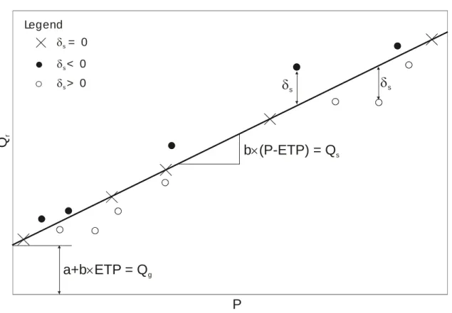
prior to any least squares fitting. Figure 2 shows a typical Q

versus P plot for a month X in the

cold-wet season. The thick line is the least squares fitting. The large crosses are points of the thick

line, meaning that all overland flow of month X contributed to the measured river flow of that

month. Contrarily, the filled circles and the open circles are plotted above and below the thick line,

respectively. In the first case (filled circles) the river flows of month X are greater than the least

squares predictions; hence the excess flows had to come from the surface water reservoir leading to

s < 0. In the second case (open circles) the river flows are smaller than the predictions, so part of

the overland flow was necessarily added to the surface water reservoir (

> 0). During the cold-wet

season, more years are expected with 

> 0 than with 

< 0, because during this season the water

levels in the rivers rise, and Median (s

) = s

> 0 is expected.

In summary, four consecutive steps are necessary to estimate Qs, Qg, s and I, in Equations 2a,b:

Step 1 – For each month, rainfall (P) has to be plotted against river flow (Q

) on a bilinear diagram.

For the present case study P and Qr listed in Appendices A and B were used.

Step 2 – Points that markedly correspond to measurement errors should be removed.

Step 3 – The other scatter points have to be fitted using the least squares method, in order to

estimate the values of parameters a and b.

Step 4 – Using medians, Qs (Equation 3), Qg (Equation 5b), s (Equation 5a) and I (Equation 2b)

may be determined. The use of medians (instead of means) is justified because precipitation, the

source for the above mentioned water balance components, is distributed irregularly in time and

therefore requires a more robust estimate of its central tendency value.

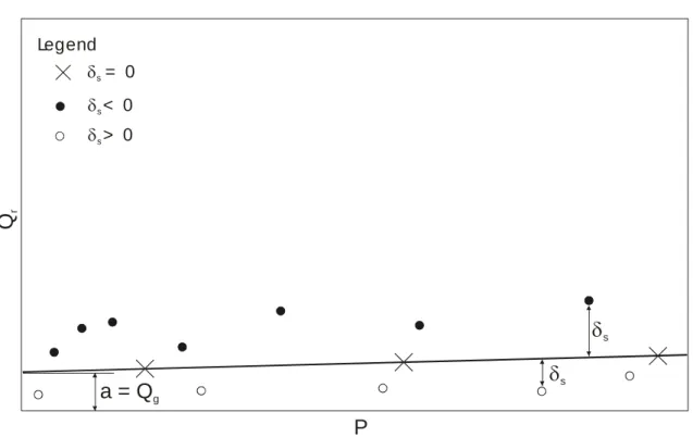
The warm-dry season - Usually, the warm-dry season is a period of water deficit (P< ETP).

During this period, most rainfall is consumed by direct evaporation from interception, and therefore

only a negligible portion of P is converted into overland flow (i.e. Qs  0) or infiltration (I  0).

River flows are of almost exclusive underground origin, and for that reason plots of Q

versus P

usually give points around straight-lines of low slope (b  0). Similarly to the cold-wet season,

Figure 3 illustrates the typical relationship between Qr and P for a month in the warm-dry season.

Equations for the warm-dry season are derived readily from those of the cold-wet season, taking

into account the current assumptions (Qs = 0 and I = 0) and the usual observations (b  0). Equation

5b can be rewritten as:

Q

 a

(6a)

and Equation 5a as:

s  a  Qr

(6b)

Contrarily to the cold-wet season, 

< 0 is expected, in agreement with the lowering of river water

levels.

ET

is an important water-balance component during the warm-dry period, but standing solely on

P, Qr and ETP records it is not possible to estimate ETm on a monthly basis. Nevertheless, if the

underground reservoir is assumed to be in steady-state on an annual basis (annual g = 0), then the

annual ET

can be calculated on that basis using Equation 1c (ET

= I – Q

).

STUDY AREA

The hydrographic basin of Corgo river is located near Vila Real (north of Portugal) and has an area

of approximately 290 km

(Figure 4). Altitudes vary between 60 m in the mouth and 1360 m in the

spring. For a river that is approximately 40 km long, this represents an average riverbed slope of

3.2%.

The Corgo river is an affluent of the Douro river and runs mostly along a large-scale tectonic

depression, the so-called PenacovaRéguaVerin fault. The geology of the basin is characterized by

Paleozoic metassediments that were intruded by Hercynian granites and covered locally by

Quaternary deposits (Sousa, 1982; Matos, 1991). Major soil types are luvisols (53 %), anthrosols

(22 %) and leptosols (9 %), with thicknesses that usually do not exceed 80 cm. Land use is

dominated by forests (pine, oak, eucalyptus) intermixed with agricultural areas. In the highlands,

the earth surface is covered mostly by spontaneous vegetation, while in the tectonic valleys there is

a predominance of agriculture.

The region is characterized by a cold-wet period running from October to May, succeeded by a

warm-dry period lasting from July to August. Although they vary considerably in their temperatures

and precipitations, the months of June and September can be included in a warm-wet period (Figure

5). The river flows reflect the climatic conditions, with the periods of high and low runoff

coinciding with the cold-wet and warm-dry seasons, respectively.

Precipitation and river flow data

Representative precipitation data were computed for a drainage area inside the Corgo river basin

from the records of 7 meteorological stations (Figure 6) using the Thiessen polygons method. For

the period 1960/611984/85, results are summarized in Appendix A. River flow data of the same

period were obtained at the Ermida hydrometric station (Figure 6) and are compiled in Appendix B.

RESULTS AND DISCUSSION

Q

versus P regressions and error analysis

Using the data in Appendices A and B, Qr versus P scatter plots were drawn for all months in a year

and the corresponding least squares fittings were calculated (Table 1). Prior to the calculation of

these fittings, some markedly anomalous points (e.g., associated with measurement errors in Q

and/or P) were removed from the plots; in total 17 out of 300 points (5.6%). The cold-wet period

(PETP > 0) includes all months from October to May, the warm-dry period (PETP < 0) the

remaining months. As expected, the scatter points fit to straight-lines of high slope for the months

in the cold-wet period (median b = 0.50) and to straight-lines of low slope for the months in the

warm-dry period (median b = 0.12). The associated coefficients of determination (r

) are 0.8 and

0.3, respectively.

Water balances

The water balance components were calculated on a monthly basis, using medians of precipitation

(P), river flow (Qr) and potential evapotranspiration (ETP), in combination with the a and b

coefficients deduced from the Q

versus P regressions (Table 1). The P and Q

medians were

determined from data in Appendices A and B, the ETP medians by the Thornthwaite method, using

long-term average temperatures as given in INMG (1991).

The calculated components of the water balance (Qg, Qs, Δs, I) are also shown in Table 1. On a

yearly basis, infiltration approaches I = 346 mm and base flow Qg = 303 mm. Assuming that the

underground reservoir is in steady-state on a yearly basis (g = 0), then the difference between I and

Q

(43 mm) is the annual ET

(Equation 1c). This value is consistent with the 75 mm obtained by

Alencoão (1998) for a nearby basin.

Seasonal variations of water balance components

The calculated infiltrations (I), surface and base flows (Qs, Qg), and changes to the surface water

reservoir (s

), for each month in a year, are shown in Figure 7 (source data taken from Table 1). As

expected, infiltration occurs during the cold-wet season, especially in the period

NovemberJanuary, and generally speaking is out of phase with the base flow, which is more

important in the period MarchMay. The lag phase of maximum I and maximum Qg is tg = 4

months.

From October to January infiltration increases rapidly, while the base flows are kept relatively low

(except in January), meaning that the underground reservoir is being replenished (g > 0).

Eventually, some saturation occurs in January, which would explain the decrease in I during

February. In response to a refill of the underground reservoir, the base flows increase rapidly from

January till March, and stay high till May. In February and upcoming months I < Q

. Consequently,

g

< 0 and infiltration may increase again, which occurs in March. The period MarchJune is

characterized by a progressive decrease in infiltration, caused by a decline in the rainfall. For the

same time span there is a progressive decrease in the base flow, which is related to the normal

emptying of the underground reservoir. Finally, from July to September, infiltration remains at the

zero level and base flows are reduced to residual values.

The accumulated change to the surface water reservoir is represented in Figure 7 by the thick line.

During the cold-wet season, 

> 0 and therefore the accumulated 

grows gradually till reaching a

value close to 26 mm in May. This result is consistent with the normal rise of the river’s water level

during the winter and spring seasons. From June on s < 0 and so the accumulated s drops down

till a residual value of 0.5 in September; the highest drop (22 mm) occurring in the first month of

the warm-dry period (June). In the period OctoberJanuary, the accumulated 

grows in phase with

Q

and Q

, continues rising in the period FebruaryMay notwithstanding the drop in Q

observed

after January, and drops down in June in phase with Qg, suggesting that the river’s water level is

more sensitive to the changes in Q

.

Application of the model to a nearby catchment for comparison of results

Comparison of I, R and Q

with the results obtained by other groups

Maxey and Eakin (1950), working in Nevada, USA, developed an empirical step function whereby

the annual R is set to percentages of the annual P ranging from 0 % (for P < 203 mm) to 25 % (for P

> 507 mm). Although slightly modified (R = 0 was set to P < 100 mm), the step function of Maxey

and Eakin (1950) was also used by Hevesi and Flint (1998), with consistent results. In the Corgo

river basin, P = 1202 mm and therefore R = 0.25  P, in keeping with the above mentioned step

functions. With the model introduced in this study it was found that R =303 mm, or R = 0.252 × P,

which is acceptable.

Using the Kille method (Kille, 1970), Mihálik and Kajan (1990) found Q

(annual) = 195 mm for P

(annual) = 1078 mm (thus, Q

= 0.18  P). Our results compare modestly with this but match those

of Gurtz et al. (1990) that found Qg (annual) =237 mm by continuous hydrograph separation,

meaning that Qg = 0.25  P for P (annual) = 931 mm.

In a study carried out in France, Cosandey and Didon-Lescot (1990) calculated infiltration in the

context of flood analysis, and found I (annual) = 294.4 mm for a P (annual) = 1900 mm (I = 0.15 

P). This deviates from our result (I = 0.29  P) but a reason exists for the discrepancy: at the La

Latte basin (south of the Lozére mountain) precipitation is rather irregular, with some events

producing large amounts of rain in short periods of time (e.g. 400 mm in 48 hours). This does not

occur in the Corgo basin. However, the discrepancy may also be due to a scale effect (the Latte

basin is very much smaller than the Corgo basin).

CONCLUSIONS

The model presented in this study is simple but effective. Based on a limited amount of data

(precipitation and runoff records and average potential evapotranspiration) and on the link between

precipitation and runoff, the method is able to discriminate among most terms of a water balance at

the catchment scale. Additionally, because the method estimates infiltration and base flow in

separate and on a monthly basis, the lag phase of maximum infiltration and maximum base flow is

also evaluated.

ACKNOWLEDGEMENTS

REFERENCES

Alencoão, A. M. P. (1998). Os recursos hídricos na bacia hidrográfica do rio Pinhão. PhD thesis,

Trás-os-Montes e Alto Douro University, Vila Real, Portugal

Belan, R.A., Matlock, W.G. (1973). Groundwater recharge from a portion of the Santa Catalina

Mountains. In: Hydrology and water resources in Arizona and the Southwest Arizona Section,

3340. Rep. 3, American Water Resources Association, and the Hydrology Section, Arizona

Academy of Science, Tucson, Arizona, USA.

Beven, K.J. (2001). Rainfall-Runoff Modelling. J. W. and Sons. Chichester, England.

Ciarapica, L., Todini, E. (2002). TOPKAPI: a model for the representation of the rainfall-runoff

process at different scales. Hydrol. Processes 16, 207–229.

Cook, P.G., Hatton, T.J., Pidsley, D., Herczeg, A.L., Held A., O'Grady, A., Eamus, D. (1998).

Water balance of a tropical woodland ecosystem, northern Australia: a combination of

micro-meteorological, soil physical, and groundwater chemical approaches. J. Hydrol. 210,

161177.

Cook, P.G., Herczeg, A.L., McEwan, K.L., (2001). Groundwater recharge and stream baseflow,

Atherton Tablelands, Queensland. CSIRO Land Water Tech. Rep. 08/01.

Cosandey, C., Didon-Lescot (1990). Étude des crues cévenoles: conditions d'apparition dans un

petit bassin forestier sur le versant sud du Mont Lozère, France,. In : Regionalization in

hydrology, 103

115. IAHS Publ. 191, IAHS Press, Wallingford, UK.

Custodio, E., Llamas, M.R., (1983). Hidrología subterránea. Ediciones Omega, Barcelona, Spain.

Dawdy, D.R., O'Donnell, T. (1965). Mathematical models of catchment behavior. Proc. ASCE HY4,

v. 91, 123



137.

Gee, G.W., Hillel, D. (1998). Groundwater recharge in arid regions: review and critique of

estimation methods. Hydrol. Processes 2, 255266.

DGRAH  Direcção Geral dos Recursos e Aproveitamentos Hidráulicos (1986). Dados

pluviométricos, 1900/01 a 1984/85, Portugal Continental. DGRAH, Lisboa, Portugal.

Flint, A. L. , Flint, L. E., Hevesi, J. A., D'Agnese F. A., Faunt, C. C. (2000). Estimation of regional

recharge and travel time through the unsaturated zone in arid climates. In: Dynamics of fluids

in fractured rock (ed. by Faybishenko B., Witherspoon, P., Benson, S. ) , 115

128.

Geophysical Monogr 122, American Geophysical Union, Washington DC, USA.

Flint, A. L. , Flint, L. E., Kwicklis, E. M., Fabryka-Martin, J. T., Bodvarsson, G. S. (2002).

Estimating recharge at Yucca Mountain, Nevada, USA: comparison of methods.

Hydrogeology Journal 10, 180

204.

Gurtz, R., Schwarze, Peschke, G., Grunewald, U., (1990). Estimation of the surface, subsurface and

groundwater runoff components in mountainous areas. In: Hydrology of mountainous areas,

263280. IAHS Publ. 190, IAHS Press, Wallingford, UK.

Halford, K.J., Mayer, G.C. (2000). Problems associated with estimating ground water discharge and

recharge from stream-discharge records. Ground Water 38, 331342.

Hendrickx, J., Walker, G. (1997). Recharge from precipitation. In: Recharge of phreatic aquifers in

(semi-)arid areas (ed. by I. Simmers), 19

98. A A Balkema, Rotterdam, The Netherlands.

Hevesi, J.A., Flint, A.L. (1998). Geostatistical estimates of future recharge for the Death Valey

Region. In: Proc. 9

Int. High-Level Radioactive Waste Manage Conf., Las Vegas, Nevada,

173177. Americal Nuclear Society, LaGrange Park, Illinois.

INMG  Instituto Nacional de Meteorologia e Geofísica (1991). O clima de Portugal, Fascículo

XLIX, v. 3, 3ª região. INMG, Lisboa, Portugal.

Jonch-Clausen, T. (1979). SHE, Système Hydrologique Européen. A short description. Danish

Hydraulic Institute.

Kille, K. (1970). Das Verfahren MoMNQ, ein Betrag zur Berechnung der mittleren lang-jährijen

Grundwasser-neubildung mit Hilfe der monatlichen Niedvigwassarab-flüsse. Zeitschrift d.

Deutsch. geol. Gesselschaft, Sonderheft Hydrogeologie und Hydrochemie, 8995.

Lerner, D. N. (1997). Groundwater recharge. In: Geochemical processes, weathering and

groundwater recharge in catchements (ed. by O. M.Saether and P. de Caritat), 109

150. A A

Balkema, Rotterdam, The Netherlands.

Matos, A.V. (1991). A geologia da região de Vila Real. Ph.D. Thesis, Trás-os-Montes e Alto Douro

University, Vila Real, 312p.

Maxey, G.B., Eakin, T.E. (1950). Groundwater in White River Valey, White Pinh, Nye, and Lincon

Counties, Nevada. NV State Eng. Water Resour. Bull. 8, 159.

Mihálik, F., Kajan, J. (1990). Groundwater runoff in mountainous areas of Slovakia and its relations

to precipitation and hydrogeological conditions. In: Hydrology of mountainous areas,

313327. IAHS Publ., 190, IAHS Press, Wallingford, UK.

Pacheco, F.A.L. & Van der Weijden, C. H. (2002). Mineral weathering rates calculated from spring

water data: a case study in an area with intensive agriculture, the Morais massif, NE Portugal.

Appl. Geochem. 17(5), 583

603.

Pacheco, F.A.L. & Alencoão, A.M.P. (accepted). Role of Fractures in Weathering of Solid Rocks:

Narrowing the Gap Between Experimental and Natural Weathering Rates? J. Hydrol.

Ronan, A. D., Prudic, D.E., Thodal, C.E. Constanz, J. (1998). Field study and simulation of diurnal

temperature effects on infiltration and variably saturated flow beneath and ephemeral stream.

Water Resour. Res. 34, 2137

2153.

Rosenberry, D.O. (2000). Unsaturated-zone wedge beneath a large natural lake. Water Resour Res.

36, 3401

3409.

Scanlon, B. R., Tyler, S.W., Wierenga (1997). Hydrologic issues in arid systems and implications

for contaminant transport. Rev. Geophys. 35, 461490.

Scanlon, B. R., Healy, R. W., Cook, P. G. (2002). Choosing appropriate techniques for quantifying

groundwater recharge. Hydrogeology Journal 10, 1839.

Sousa, M.B., (1982). Litoestratigrafia e estrutura do "Complexo Xisto-Grauváquico

ante-Ordovícico"  Grupo do Douro (Nordeste de Portugal). PhD Thesis, Coimbra University,

Coimbra, Portugal.

Thornthwaite, C.W., Mather, J.R., (1955). The water balance. Publ. Climatol. Lab. Climatol. Drexel

Inst. Technol., v. 8, 1



104.

Todini, E., (1996). The ARNO rainfall-runoff model. J. Hydrol 175, 339382.

Van der Weijden, C.H., Pacheco, F.A.L. (2003). Hydrochemistry, weathering and weathering rates

on Madeira island. J. Hydrol. 283(1-4), 122145.

Verhagen, B.T. (1992). Detailed geohydrology with environmental isotopes. A case study at

Serowe, Botswana. In: Isotope techniques in water resources development, 345362.

International Atomic Energy Agency, Vienna.

Xiong, L., Guo, S. (1999). A two-parameter monthly water balance model and its application. J.

Hydrol. 211, 111

123.

Xu, C.-Y., Singh, V.P. (1998). A review on monthly water balance models for water resources

investigations. Water Resources Management 12, 31–50.

Xu, C.-Y., Singh, V.P. (2004). Review on regional water resources assessment: models under

stationary and changing climate. Water Resources Management 18, 591–612.

TABLE 1

Legend: Input data for the water balance (columns below the "Data” heading), results of the least

squares fittings (columns under the heading "Least Squares Regressions") and calculated

components of the water balance (columns under the heading “Water Balances”).

Month

Data Least Squares Regressions

P-ETP Water Balances P Qr ETP Anomalous Years a b r 2 Qg Qs s I Oct 96.9 13.5 61.8 1,2,17,22 -4.96 0.20 0.80 35.1 7.4 7.0 0.9 28.0 Nov 125.8 41.7 27.4 17,25 0.15 0.34 0.80 98.4 9.5 33.4 1.2 64.9 Dec 180.7 116.9 17.5 2.69 0.65 0.91 163.2 14.1 106.1 3.3 57.1 Jan 218.6 159.4 17.9 5 22.55 0.66 0.69 200.7 34.4 132.4 7.4 68.2 Feb 148.1 127.7 18.3 25.51 0.72 0.73 129.8 38.7 93.4 4.4 36.3 Mar 121.4 96.2 35.2 3,4,9,18,19 50.68 0.42 0.75 86.2 65.5 36.2 5.5 50.0 Apr 111.5 88.1 49.9 40.57 0.44 0.62 61.6 62.5 27.1 1.5 34.5 May 92.1 60.6 76.8 10.73 0.56 0.79 15.3 53.7 8.6 1.7 6.7 Jun 44.9 33.1 105.0 14 10.78 0.43 0.48 -60.1 10.8 0.0 -22.4 0.0 Jul 9.0 5.7 133.4 14 3.96 0.19 0.28 -124.4 4.0 0.0 -1.7 0.0 Aug 9.9 1.4 120.7 11,13,14 1.46 0.01 0.01 -110.8 1.5 0.0 0.0 0.0 Sep 43.0 2.5 90.6 1.17 0.04 0.37 -47.6 1.2 0.0 -1.3 0.0 Total 1201.7 746.8 754.5 303.1 444.2 0.5 345.8

P  median precipitation after excluding the anomalous years; Q

 median river flow after

excluding the anomalous years; ETP  potential evapotranspiration; a, b  intercept-y and slope of

the regression line; r

 associated coefficient of determination; Qg  base flow; Qs – overland flow;

s – change to the surface water reservoir; I  infiltration. All columns under the “Data” and “Water

Balances” headings are in mm. Numbers under the heading “Anomalous Years” are in agreement

with the Nr codes in Appendices A and B.

FIGURE 1

Hydrographic Basin:

surface (_s) and underground _gwater

reservoirs I P E_p Q_s Q_g Q_r ET_m E_r

Caption: The water balance at the catchment scale. Symbols (units are in mm): P

 precipitation; Er

 evaporation from the river channel; ETm  evapotranspiration from the soil and organic

compartments; Ep  direct evaporation; I  infiltration; Qs  overland flow; Qg  base flow; Qr 

river flow.

FIGURE 2

Q

P



a+b



ETP

= Q



b (P-ETP) = Q



Caption: Schematic representation of a typical Q

period. Symbols (units in mm, except for b that is dimensionless): P  precipitation; Qr  river flow;

Qg  base flow; Qs – overland flow; ETP  potential evapotranspiration; s – change to the surface

water reservoir in a particular year; a and b  intercept-y and slope of the regression line.

FIGURE 3

P

Q





a = Q

Caption: Schematic representation of a typical Q

period. Symbols (units in mm): P  precipitation; Q

 river flow; Q

 base flow; s

– change to the

surface water reservoir in a particular year; a  intercept-y of the regression line.

FIGURE 4

Portugal

Porto

Lisboa

Trás-os-Montes e Alto Douro

Bragança Vila Real 8º _7º 42º 41º 9º Legend Agriculture Forest Urban areas Uncultivated land 5.000 2.500 0m Terva basin

FIGURE 5

Caption: Strahler diagram of the Corgo river hydrographic basin. Precipitation and temperature

FIGURE 6

Caption: Topography and drainage pattern within the Corgo river basin. Location of the

hydrometric station and of meteorological stations used to calculate precipitation averages.

Boundary lines: of the Corgo basin (dash-dot line); of the drainage area upstream the hydrometric

station (dashed line).

FIGURE 7

0.0

20.0

40.0

60.0

80.0

100.0

120.0

140.0

Oct

Nov Dec

Jan

Feb Mar

Apr May

Jun

Jul

Aug

Sep

Month

mm

APPENDIX A

Nr Year

Month

Oct Nov Dec Jan Feb Mar Apr May Jun Jul Aug Sep

1 60/61 465.8 406.9 271.6 259.5 90.4 16.3 288.8 137.2 46.0 99.5 6.5 29.4 2 61/62 206.8 217.4 496.7 224.2 33.0 392.0 161.2 57.1 30.5 31.4 1.0 51.4 3 62/63 68.8 96.9 86.6 424.7 601.7 281.1 190.4 50.1 116.0 2.8 4.2 35.5 4 63/64 96.8 717.2 380.4 18.2 393.6 340.4 83.7 36.6 115.7 19.3 9.1 43.0 5 64/65 160.7 15.8 94.5 327.0 74.6 325.6 16.6 28.5 31.0 6.2 3.0 201.9 6 65/66 173.3 352.3 336.4 527.4 613.8 1.2 370.8 33.6 103.2 1.3 39.6 43.9 7 66/67 274.5 179.7 66.3 132.1 190.8 146.9 37.8 216.1 10.1 0.1 27.4 54.8 8 67/68 76.8 125.8 27.6 8.4 385.8 91.9 209.0 125.9 13.1 0.8 47.6 121.8 9 68/69 117.6 236.9 303.0 312.5 257.8 470.2 114.0 199.6 69.6 9.8 0.3 119.3 10 69/70 44.4 158.0 93.7 501.4 79.1 30.9 24.0 206.0 67.6 7.7 17.3 7.2 11 70/71 8.5 253.1 41.4 321.7 41.2 113.8 123.9 178.8 141.6 78.7 31.1 4.5 12 71/72 66.8 32.3 55.0 207.6 431.6 168.7 31.6 64.9 25.5 38.2 5.8 62.1 13 72/73 154.9 124.2 207.7 213.3 27.4 25.6 58.6 184.4 35.9 37.7 12.0 44.0 14 73/74 136.3 30.6 101.0 382.6 236.7 54.7 23.1 86.0 262.3 2.7 1.1 33.9 15 74/75 5.9 197.4 37.4 226.1 147.9 204.5 35.2 36.5 7.7 1.5 12.7 142.9 16 75/76 96.9 99.0 59.2 73.2 76.6 71.9 63.6 9.6 38.8 33.1 79.2 95.9 17 76/77 265.5 130.3 283.2 378.1 445.4 129.0 74.0 65.4 74.7 13.7 34.2 27.1 18 77/78 170.8 99.0 352.3 223.8 477.8 160.6 168.1 91.9 66.2 3.6 0.0 11.6 19 78/79 42.7 47.4 743.9 204.9 478.5 236.9 164.0 94.0 4.3 19.7 1.1 10.9 20 79/80 276.4 77.8 180.7 125.8 113.6 138.3 54.5 115.5 43.8 14.4 10.8 32.9 21 80/81 62.3 112.2 50.4 2.4 92.8 158.6 129.5 117.1 21.6 7.9 8.8 121.9 22 81/82 144.4 0.0 589.6 120.3 83.7 7.1 56.1 49.1 47.7 8.2 18.7 108.6 23 82/83 118.2 195.3 216.2 15.5 148.1 23.4 367.2 299.4 42.7 15.3 41.9 7.5 24 83/84 47.1 199.0 290.4 187.6 35.9 192.7 111.5 106.3 91.3 7.9 30.5 40.6 25 84/85 212.9 382.8 125.2 273.5 277.3 133.2 124.4 92.1 57.4 8.0 1.0 7.3

Legend: Monthly precipitation (P in mm) at the Corgo river hydrographic basin, covering the

APPENDIX B

Nr Year

Month

Oct Nov Dec Jan Feb Mar Apr May Jun Jul Aug Sep

1 60/61 165.5 88.9 192.2 191.4 87.7 42.1 98.3 60.6 28.8 8.1 2.0 1.2 2 61/62 8.9 55.2 251.1 232.5 47.4 191.7 144.5 40.1 13.5 2.9 0.8 0.3 3 62/63 1.0 3.4 10.4 129.6 262.4 360.0 142.6 46.4 46.6 6.4 1.9 1.8 4 63/64 4.2 261.3 207.1 59.9 191.2 373.6 84.6 37.4 38.9 6.1 1.5 1.0 5 64/65 13.5 7.9 12.5 85.7 67.0 202.6 45.7 23.2 6.6 0.4 0.0 11.0 6 65/66 32.4 174.2 235.6 416.5 537.3 90.5 226.7 54.3 38.0 4.9 0.6 0.0 7 66/67 40.4 91.9 48.8 70.0 127.7 101.8 38.6 99.7 26.9 4.6 1.0 0.0 8 67/68 0.3 30.3 14.9 12.5 152.7 84.3 102.5 101.3 17.9 2.7 0.8 13.1 9 68/69 15.0 116.4 262.5 257.5 203.9 371.3 105.6 148.1 63.9 14.8 2.1 10.5 10 69/70 12.5 41.3 43.7 398.5 122.6 52.2 34.2 84.3 33.4 5.3 1.6 1.5 11 70/71 1.7 31.1 32.7 198.4 79.5 104.0 79.5 99.4 112.7 46.2 16.1 5.7 12 71/72 9.8 7.7 12.7 89.1 345.4 157.8 50.2 41.7 14.2 4.5 0.8 3.9 13 72/73 21.2 58.1 116.9 204.3 54.5 32.6 23.8 98.0 39.5 12.3 5.1 5.7 14 73/74 23.9 17.1 35.0 222.9 237.7 71.3 43.3 50.0 99.2 40.8 4.7 6.0 15 74/75 4.9 41.7 28.8 96.7 123.0 166.9 48.1 31.1 12.6 1.8 0.3 3.8 16 75/76 16.9 32.3 47.8 30.9 67.5 52.2 40.6 19.6 4.2 2.9 1.4 3.2 17 76/77 131.4 143.9 244.3 354.8 456.0 154.0 98.1 48.2 35.0 11.0 3.8 2.8 18 77/78 40.5 48.7 275.6 189.1 425.8 224.5 88.1 86.8 32.8 10.5 3.0 2.5 19 78/79 2.4 4.8 473.0 251.9 570.1 376.4 210.8 67.4 31.4 6.8 2.0 1.5 20 79/80 64.8 61.0 99.8 127.7 128.7 104.1 78.4 87.0 33.5 6.6 2.6 2.4 21 80/81 10.4 41.3 28.7 20.0 24.7 80.6 112.5 81.7 29.4 5.0 0.5 5.3 22 81/82 83.5 9.7 383.4 78.5 78.6 52.5 33.0 18.0 7.2 0.9 0.1 0.8 23 82/83 21.7 81.8 170.5 69.8 69.8 55.0 177.9 230.0 55.5 7.9 3.4 2.2 24 83/84 3.6 55.8 235.4 83.6 83.6 111.6 123.4 90.2 64.3 8.9 3.1 3.0 25 84/85 47.9 280.0 176.1 338.5 338.5 144.8 140.3 47.6 38.9 4.2 1.1 0.9

Legend: Monthly river flows (Q

during the period 1960/611984/85. Source data retrieved from www.inag.pt.