A W
ORKP
ROJECT,
PRESENTED AS PART OF THE REQUIREMENTS FOR THEA
WARD OF AM
ASTERD
EGREE INF
INANCE FROMNOVA - S
CHOOL OFB
USINESS ANDE
CONOMICS.
I
S THERE A LOW
-
RISK PREMIUM
IN COMMODITY MARKETS
?
F
ELIX
B
RUNNER
, 973
A P
ROJECT CARRIED OUT ON THEM
ASTER INF
INANCEP
ROGRAM,
UNDER THE SUPERVISION OF
M
ARTIJN
B
OONS
, P
H
D
Abstract
This paper examines the existence of a low-risk anomaly in the asset class of commodity fu-tures. Using dynamic market betas as ranking variable for sorted portfolios, results indicate that significant factors can be constructed by slightly altering the parameters used in previous literature. When additional asset-specific risk measures are incorporated to sort assets into long-short portfolios, especially low-drawdown portfolios yield abnormal returns with regards to the benchmarks. Although not constituting an anomaly, findings on the compensation of tail risks in the form of kurtosis, that consistently showed up significant throughout robustness tests, are also reported.
Keywords: Commodity futures returns, cross-sectional asset pricing, low risk anomaly, alter-native risk premia
1
Introduction and Theoretical Motivation
Evidence for the low-risk effect in its various forms reaches back as far as 1972, when Jensen et al. (1972) indicate that the expected excess return on an asset is not strictly proportional to its beta, with high-beta stocks having negative alphas and low-beta stocks having positive al-phas. Similarly, Fama and French (1992) observe a slight decline of average monthly returns on sorted stock portfolios with increasing betas. This constitutes a puzzle to investment theory as it challenges the traditional equilibrium asset pricing framework initially set by Sharpe (1964), where higher-risk securities are rewarded with higher expected returns. Either this relationship just does not hold, or additional risks have to be accounted for in the models.
A multitude of factors have been proposed, with prominent examples being size and value in equities, and term and default in fixed income (see Fama and French (1992), Fama and French (1993)), momentum in many asset classes (see Jegadeesh and Titman (1993), Carhart (1997), Moskowitz et al. (2012)), liquidity in equities (see Pastor and Stambaugh (2001), Ami-hud (2002), Sadka (2006)), carry in many asset classes (see Koijen et al. (2013)), and investment and profitability in equities (see Titman et al. (2004), Novy-Marx (2013), Fama and French (2015)). Many more factors have been suggested in academia, with an aggregate study of McLean and Pontiff (2016) surveying as much as 97 previously reported long-short return pre-dictors, and Harvey et al. (2015) listing 313 published papers that study cross-sectional return patterns. This high count alone leaves doubts on the validity of the reported factors as pricing benchmarks and their robustness has to be questioned. Only a fraction of the alleged return patterns have been validated in various asset classes, with the low-risk effect being one.
A whole area of literature has evolved around harnessing such alternative return premi-ums as investment strategies (see for example Barberis and Shleifer (2003), Litterman (2008), Carhart et al. (2014)). In combining only well-tested factors, Asness et al. (2013a) introduce an approach to diversify into alternative return factors by building market-neutral portfolios. They identify four systematic long-short investment methods that yield long-term positive average returns across geographical markets and asset groups, with low correlation to long-only market indices. Further, they require in-sample and out-of-sample scientific evidence, and a credi-ble underlying economic story in the risk and behavioural literature. Using this definition, the
before mentioned dubiousness of factor robustness is minimised. The asset classes for imple-mentation of the strategies in this paper are individual stock selection, equity industry selection, equity country selection, government bond futures, interest rate futures, currency futures and commodity futures. However, they are not able to implement all of their four systematic strate-gies (value, momentum, carry and defensive) in all asset classes. Israel and Maloney (2014) revisit the exact same factors and provide further evidence on the diversification benefits of such investments.
The factor ’defensive’ is a systematic exploitation of the low-risk effect as previously re-ported. With the pricing irregularities in standard models already known, Ang et al. (2006) ex-amine the cross-sectional pricing of exposure towards aggregate volatility innovations in the US equity market and document low average returns for stocks with high sensitivities. Further, they find a highly significant relation of idiosyncratic volatility relative to the Fama/French 3-Factor Model (Fama and French (1992)) and the cross-section of returns. This anomaly is only frac-tionally explained by the volatility innovation factor. The authors then test the robustness of this anomaly by controlling for other known anomalies and risk premiums, and by demonstrating the persistence across different sub-samples of different periods, economic cycles and volatility environments. Blitz and Van Vliet (2007) provide further evidence in the US, European and Japanese equity markets. However they sort into portfolios based on three-year realised volatil-ities instead of short-term 1-month measured volatility. Additionally, an important finding of their paper is that ranking equities on their realised volatility resembles ranking equities based on ex ante betas, i.e. both ranking methods reflect a similar underlying phenomenon.
Baker et al. (2011) maintain that volatility and beta are highly positively correlated and that volatility-sorted portfolios are very similar to beta-sorted portfolios. They also extend the low-risk literature towards additional asset classes as their computations include government bonds and corporate bonds, along with the frequently studied stock markets. Frazzini and Pedersen (2014) focus on beta-ranked portfolios and include even more asset classes, one of which are commodity futures. However, they are not able to reject the hypothesis of zero average returns for the strategy in this asset class. Instead, they present a low-beta strategy that includes futures on all kind of underlyings and delivers significant abnormal returns of 0.26 percent per month.
Literature gives a number of theories for why the low-risk anomaly exists and why low risk assets outperform riskier assets on a risk-adjusted basis, even after the effect became widely known. Blitz et al. (2013) offer an overview of explanations, where the most common reasoning is leverage-aversion or leverage-constraints that force investors to crowd into riskier assets to meet their risk and return expectations (see Ang et al. (2006), Frazzini and Pedersen (2014)). However, it is questionable whether this explanation is applicable in the futures asset class, where all available assets are leveraged by definition. Other explanations include regulatory constraints, constraints on short-selling, relative utility, agents being willing to pay for volatility as it increases the option-like pay-off structures of their mandates, preference for skewness, and crash aversion leading to more similar subjective risk evaluations than pricing models suggest.
Different markets and geographies are subject to different systematic pricing patterns, and therefore pertain different risk factors. Yet, most academic and non-academic literature focusses on US equities. Some studies have tried to transfer concepts towards other asset classes and the extensive literature on the low-risk effect bears testimony for its robustness across time, geographies and markets. In spite of this extension of the concept into the commodity futures market, the evidence in that particular market remains thin. While other systematic factors such as value, momentum and carry have been successfully replicated in data sets that contain commodity futures returns (see Asness et al. (2013a), Israel and Maloney (2014)), low-risk investing in commodities remains a gap in academic literature.
This paper aims at helping to close this gap by offering a rationale how low-risk strategies can be implemented in commodities. This amends both the literature on the low-risk effect and on the commodity market. Consequently, the presented findings can potentially help to develop better pricing models for that particular market, and to implement investment strategies that take advantage of the low-risk effect in the commodities market. The hypothesis to test is that a long-short investment strategy based on ranking by riskiness of asset can produce significant abnormal returns in the asset class of commodity futures.
The rest of this paper is organised as follows. Section 2 summarises the data set and de-scribes the sources of data. Section 3 explains the methodology of estimating risks and using that information to form portfolios. Section 4 discusses the empirical support of the findings.
Section 5 concludes and summarises the results. Appendix A contains details of the data set and Appendix B shows definitions and specifics of the used risk estimators.
2
Data and Summary Statistics
The main dataset used in this analysis is identical to the one used in Boons and Prado (2015) and consists of one-day returns on exchange-traded, liquid commodity futures contracts col-lected from the Commodity Research Bureau and the Futures Industry Institute reaching back to July 1959 and ending in January 2015. Each daily return corresponds to holding the most liquid futures contract on the underlying commodity from market open to close. On a monthly frequency, the same method is used with a one-month holding period. All returns are in US dollars. The sample contains a total of 32 different commodity futures, where not all assets are traded at all times. On average, 24.29 assets are available per return period, with almost the full data set starting to be available in the subsample from 1990 (a detailed list can be found in Table 6 in Appendix A). For each asset, there are 10,642 daily observations and 508 monthly observations available on average.
Some of the below explained calculations require the inclusion of additional data, and also for evaluation purposes of the results, complementary data is matched and added to the data set. As a proxy for the return of a risk free asset, the US Treasury bill rate is used. For the purpose of the standard factor models, the market excess-, size-, value- and momentum-factor
returns following the methodology of Fama and French (1992) are added to the data1. With the
focus of this study being commodity markets, these factors may not be the most compelling benchmarks for our resulting portfolios. Hence, the construction of a directly related market factor is described below. To amend this constructed factor and set up a three factor model in commodities, the value and momentum in commodities factors of Asness et al. (2013b) are also
added to the data set in periods of availability2. The factor data is also described in more detail
for each time series in Table 6 in Appendix A.
1All four factors are from Ken French’s online data library and can be downloaded from:
http://mba.tuck.dartmouth.edu/pages/faculty/ken.french/data library.html
2The commodity factors are from Lasse Pedersen’s online data library and can be downloaded from:
3
Methodology and Definitions
3.1
Estimation of Asset-Specific Risk
Based on the work of Frazzini and Pedersen (2014), the here used methodology starts with estimating asset-specific risks on a rolling window of past return data. However, we not only estimate betas towards a market index as in their paper, but also use other notions of risk as previous research has shown significant effects when building portfolios based on idiosyncratic asset volatility or sensitivity towards shocks in market volatility (see Ang et al. (2006)). There-fore, it is likely that the inclusion of different estimation techniques of asset-specific risk can yield additional insights. An overview of what measures have been estimated can be found in Table 1 in Appendix B. While it is true that many of those risk measures are likely to approxi-mate the exact same risk characteristics of the assets, some may still be more accurate or suitable in a specific market, such as the here examined commodities futures market. Most risk measures can simply be calculated from historical return data. As a market proxy, an equal-weighted in-dex is constructed out of the available futures returns at each time period. The first differences of this index’ volatility then serves as a proxy for innovations to the aggregate volatility in the commodities futures market following Ang et al. (2006). Some more complex approaches re-quire the inclusion of additional time series data from the above described sources. The data used to calculate each risk measure is also specified in Table 1.
With return data being available at both daily and monthly frequency, eleven different set-ups for the rolling estimation window (which could also be considered as the formation period) are estimated. For each estimation set-up, there is a minimum number of observations required within each window to avoid having big differences in the risk estimation across assets, and also to prevent outliers resulting from few observations. A summary of the used parameters is given in Table 7 in Appendix B. Additionally, to follow Frazzini and Pedersen (2014), robust market betas have been estimated as
ˆ βi = ˆρ ˆ σi ˆ σm (1)
where correlation ˆρ is estimated on daily data using five years of observations, and volatilities
ˆ
control for non-synchronous trading when estimating correlations as the data set is not subject to time differences.
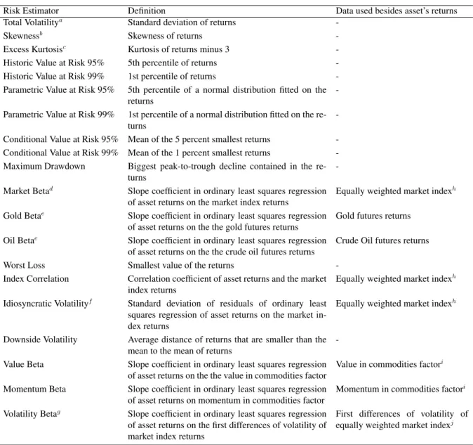
Table 1: Risk estimators of asset specific risk with definition and additional data that was used in the estimation of each estimator
Risk Estimator Definition Data used besides asset’s returns Total Volatilitya Standard deviation of returns
-Skewnessb Skewness of returns
-Excess Kurtosisc Kurtosis of returns minus 3
-Historic Value at Risk 95% 5th percentile of returns -Historic Value at Risk 99% 1st percentile of returns -Parametric Value at Risk 95% 5th percentile of a normal distribution fitted on the
returns
-Parametric Value at Risk 99% 1st percentile of a normal distribution fitted on the re-turns
-Conditional Value at Risk 95% Mean of the 5 percent smallest returns -Conditional Value at Risk 99% Mean of the 1 percent smallest returns -Maximum Drawdown Biggest peak-to-trough decline contained in the
re-turns
-Market Betad Slope coefficient in ordinary least squares regression
of asset returns on the market index returns
Equally weighted market indexh
Gold Betae Slope coefficient in ordinary least squares regression
of asset returns on the the gold futures returns
Gold futures returns
Oil Betae Slope coefficient in ordinary least squares regression
of asset returns on the the crude oil futures returns
Crude Oil futures returns
Worst Loss Smallest value of the returns -Index Correlation Correlation coefficient of asset returns and the market
index returns
Equally weighted market indexh
Idiosyncratic Volatilityf Standard deviation of residuals of ordinary least
squares regression of asset returns on the market in-dex returns
Equally weighted market indexh
Downside Volatility Average distance of returns that are smaller than the mean to the mean of returns
-Value Beta Slope coefficient in ordinary least squares regression of asset returns on the the value in commodities factor
Value in commodities factori
Momentum Beta Slope coefficient in ordinary least squares regression of asset returns on momentum in commodities factor
Momentum in commodities factori
Volatility Betag Slope coefficient in ordinary least squares regression
of asset returns on the first differences of volatility of market index returns
First differences of volatility of equally weighted market indexj
asee for example Ang et al. (2006), Blitz and Van Vliet (2007) and Baker et al. (2011) in equities bsee for example Chang et al. (2013) in equities
cCremers et al. (2015) find compensation for jump risk in equity futures options
dsee for example Frazzini and Pedersen (2014), Israel and Maloney (2014) in various asset classes
eAsness et al. (2013a) remark that low-risk strategies in commodities result in static long gold and short energy positions fsee for example Ang et al. (2006), Bali and Cakici (2008) and Fu (2009) in equities
gsee Ang et al. (2006) in equities
hthe equally weighted market index is the mean of asset returns available in each period ithe value and momentum in commodities factors are from Asness et al. (2013b)
jthe construction of the volatility factor follows the methodology of Ang et al. (2006) and consists of changes in the volatility of the equally weighted market index estimated in rolling
3.2
Formation of Long-Short Portfolios
In order to test whether low-risk investment strategies yield abnormal returns, long-short
strate-gies are constructed. Stratestrate-gies are rebalanced at a monthly frequency3even though inputs are
estimated on daily data in some cases. Various approaches are chosen to capture the low-risk effect in the data. In a first step, assets are ranked every month according to their risk. The nature of the used definitions of risk makes it necessary to distinguish between an ascending
and a descending order in each case4. The underlying commodities are then assigned either to
the high-risk or low-risk portfolio. Due to the small number of assets in our dataset, the unavail-ability of some can lead to significantly differing numbers of assets contained in those portfolios over time, resulting in varying concentration of risk in the portfolios over time. Therefore, to hold the concentration more constant, we also test a set-up where only the three most risky assets are in the high-risk portfolio and the three least risky assets are assigned to the low-risk portfolio.
In a next step, assets within each portfolio are weighted in three different methods that put different emphasis on the information contained in the estimated risk measure.
First, each asset is simply assigned equal weight according to
wi =
1
n (2)
where n is the number of assets contained in the respective portfolio. This does not account for the level of each asset’s risk measure. To capture this information, the two following approaches assign weights to the securities in different ways.
In the second approach, a step function is used to chose asset weights within the portfolios. The function is given by
wi = rank ∗
1 n(n+1)
2
(3) where n is the number of assets contained in the respective portfolio and rank is highest for
3There are two reasons for that. First, to ease computational intensity. And second, to increase implementability
of such strategies.
4For example, high volatility is commonly regarded as an indicator of high risk, while an asset is seen as risky
the value that is farthest from the median value across all assets. In other words, asset weights within the portfolio are linearly increasing with their rank when ranked by their positive (nega-tive) deviation from the median. That means high-risk commodities have larger weights in the high-risk portfolio, while low-risk commodities have larger weights in the low-risk portfolio. Hence, the result takes into account the relative position of the asset’s risk within the set, but not the absolute value of each estimator.
The third weighting method also considers the absolute value of the risk estimators. Weights in the high-risk (low-risk) portfolio are given by
wHi = P ρˆi− ˜ρ ˆ ρi> ˜ρ( ˆρi− ˜ρ) , when ˆρi > ˜ρ (4) and wiL= P ρˆi− ˜ρ ˆ ρi< ˜ρ( ˆρi− ˜ρ) , when ˆρi < ˜ρ (5)
where ˆρi is the risk estimator for the asset i and ˜ρ is the median of the risk estimators of all
assets. In this weighting scheme, asset weights within the high-risk (low-risk) portfolio are linearly increasing with their risk’s positive (negative) deviation from the median value of risk across assets.
To construct long-short portfolios that capture the presumed low-risk effect, the low-risk portfolio is bought and the high-risk portfolio is short-sold. So far, the weights within both the low-risk and the high-risk portfolio add up to one. Therefore, buying one and selling the other results in a zero-investment strategy that is self-financing. However, due to the concentration of risky assets in the short-sold portfolio, this strategy is likely to bear significant risk. To balance the systematic risks of the two legs and eliminate ex ante market beta exposure, both portfolios are rescaled following Frazzini and Pedersen (2014). In their approach, a beta-hedge is carried
out using the previously estimated betas towards the equally weighted market index βt. The
resulting portfolio returns are given by
rpt+1= 1 βtwLi (rt+1wiL− r f t+1) − 1 βtwHi (rt+1wiH − r f t+1) (6)
on the risk-free asset during that month. The adjustment for the risk-free rate becomes relevant as all asset’s weights do no longer necessarily sum up to zero and the financing cost has to be accounted for.
Using this method of balancing the long-leg and the short-leg of the strategy can result in extreme weights in two scenarios. First, a negative beta of the low-risk portfolio results in a
negative scaling factor5 1
βL t
, leading to short positions in all assets. Second, in case the beta of
the low-risk portfolio is close to zero, the scaling factor for the long portfolio β1L
t
is caused to be very large and drives up the leverage of the resulting portfolio. To tackle these problems, a simple leverage constraint is used to keep the total portfolio weight between -1 and 2, while maintaining zero ex ante index beta exposure. Additionally, betas are shrunk towards one prior to scaling the long and the short leg as in Frazzini and Pedersen (2014) given by
ˆ
βi = 0.6 ˆβi+ 0.4 (7)
This reduces the influence of outliers, consequently lowering the frequency with which extreme weights occur. For example, this prevents the initial betting against beta portfolio from hit-ting the leverage constraint at any time in the sample, and results in an average long position approximately half of that without beta shrinkage.
4
Discussion of Results
4.1
Betting against Risky Assets
An initial test follows the approach and parameters of Frazzini and Pedersen (2014). Betas are estimated towards an equally weighted index of commodities as in equation (1), where volatili-ties are estimated over five years, and correlation over one year of data at a daily frequency. All available assets are included in the portfolio construction and the step function as in equation (3) is used to determine portfolio weights within the long and the short leg. Betas are shrunken with a factor of 0.6 as in equation (7), before long and short leg are rescaled as in equation (6)
5Corresponds to 1 βtwL
i
Table 2: Total and risk-adjusted performance of portfolios composed on rankings according to estimated asset risk
Performance Commodity CAPM Commodity 3-Factor Model Leverage Portfolio Excess t-statistic Volatility Sharpe Alpha t-statistic Ex Post Alpha t-statistic Average Return (Excess (% p.a.) Ratio (% monthly) (Alpha) Beta (% monthly) (Alpha) Position (% p.a.) Return)
Panel A: Betting against Beta strategy following Frazzini and Pedersen (2014) with beta-hedge and mixed window estimation as in Equation (1) (full sample) Betting against Beta 0.58 0.8729 17.78 0.03 0.32 1.5633 -0.32 0.08 0.3471 0.72
Panel B: Volatility strategies following Ang et al. (2006) with risk estimations based on 1-month windows of daily data (full sample)
Betting against Volatility Beta -2.68 -0.3660 18.71 -0.14 -0.08 -0.3656 -0.02 -0.12 -0.4977 0.00 Betting against Volatility -6.19 -1.9586 17.91 -0.35 -0.39 -2.2809 -0.71 -0.34 -1.6530 0.00 Betting against idiosyncratic Volatility -5.91 -2.1767 16.19 -0.36 -0.39 -2.3915 -0.52 -0.34 -1.7919 0.00 Betting on idiosyncratic Volatility 3.50 2.1767 16.19 0.22 0.39 2.3915 0.52 0.34 1.7919 0.00
Panel C: Beta-hedged portfolios based on risk measures estimated over 3 years of daily data (full sample)
Betting against Market Beta 3.34 1.9972 17.64 0.19 0.41 2.0552 -0.25 0.10 0.4241 0.76 Betting against idiosyncratic Volatility 0.69 0.8868 15.81 0.04 0.16 0.8906 -0.04 -0.02 -0.1123 0.36 Betting against historic VaR@95% 3.52 2.1001 16.88 0.21 0.41 2.1076 -0.07 0.08 0.3806 0.51 Betting against Drawdowns 3.43 2.0759 16.63 0.21 0.40 2.0838 -0.07 0.00 -0.0078 0.33 Betting on Kurtosis 7.87 4.0903 15.59 0.50 0.73 4.0857 0.05 0.67 3.2516 -0.04
Panel D: Unhedged zero-investment portfolios based on risk measures estimated over 3 years of daily data (full sample)
Betting against Market Beta -0.72 -0.4934 20.07 -0.04 0.13 0.6790 -0.85 -0.16 -0.7588 0.00 Betting against idiosyncratic Volatility -0.68 -0.3249 16.89 -0.04 0.07 0.3593 -0.27 -0.10 -0.4794 0.00 Betting against historic VaR@95% 0.88 1.0239 18.35 0.05 0.22 1.1384 -0.48 -0.08 -0.3712 0.00 Betting against Drawdowns 1.87 1.4136 17.40 0.11 0.29 1.4798 -0.30 -0.11 -0.5315 0.00 Betting on Kurtosis 7.30 3.8390 15.59 0.47 0.69 3.8443 0.12 0.61 3.0782 0.00
Panel E: Beta-hedged portfolios based on risk measures estimated over 3 years of daily data (1959-1989)
Betting against Market Beta 11.27 3.4968 18.67 0.60 1.06 3.6388 -0.27 1.02 2.5269 0.72 Betting against idiosyncratic Volatility 2.74 1.2632 17.64 0.16 0.35 1.2495 0.05 0.25 0.6485 0.38 Betting against historic VaR@95% 9.28 2.9277 19.22 0.48 0.89 2.9227 0.00 0.72 1.7509 0.55 Betting against Drawdowns 8.02 2.6223 19.09 0.42 0.80 2.6453 -0.09 0.44 1.1438 0.39 Betting on Kurtosis 10.47 3.5295 16.92 0.62 0.94 3.5091 0.09 0.86 2.3831 0.10
Panel F: Beta-hedged portfolios based on risk measures estimated over 3 years of daily data (1990-2015)
Betting against Market Beta -4.69 -1.0746 16.14 -0.29 -0.30 -1.1237 -0.22 -0.49 -2.0015 0.80 Betting against idiosyncratic Volatility -1.52 -0.2247 13.51 -0.11 -0.06 -0.2598 -0.17 -0.19 -0.8806 0.34 Betting against historic VaR@95% -2.43 -0.5533 13.68 -0.18 -0.13 -0.5917 -0.17 -0.31 -1.4741 0.46 Betting against Drawdowns -1.37 -0.1831 13.29 -0.10 -0.04 -0.1903 -0.04 -0.27 -1.2310 0.26 Betting on Kurtosis 5.12 2.1331 13.97 0.37 0.50 2.1307 0.01 0.51 2.1402 -0.19
Bold values are significantly different from zero at the 95 percent confidence level. Excess returns take into account financing cost at the risk-free rate. The commodity CAPM uses the equally weighted market index as market benchmark. The Commodity 3-Factor Model additionally includes the value and momentum in commodities factors of Asness et al. (2013b) and can only be estimated starting in 1972 when all three factors are available. Average leverage is the mean of the net positions at every rebalancing date.
to achieve a full-portfolio ex ante market beta of zero.
Table 2 reports excess returns per year and the connected t-statistics to reflect significance of findings. Annualised volatilities and Sharpe Ratios are also shown. To indicate risk-adjusted performance, two simple factor models are estimated on the return time series of the strategies. First, an equivalent to the Capital Asset Pricing Model (see Sharpe (1964)) in commodities, where the excess return of an equally weighted index over the risk-free rate serves as market benchmark. Second, two additional factors that have proven significant in the commodity mar-kets in previous literature, value and momentum (see Asness et al. (2013b)), have been included as explanatory variables. Table 2 shows alphas with its t-statistics for both models and an ex post market beta exposure for the portfolio returns in the Commodity CAPM. At last, the av-erage investment of each strategy (which results from levering the low-risk leg and de-levering the high-risk leg to reduce systematic market exposure) is shown for each strategy.
The initial ’Betting against Beta’ Portfolio as described above is shown in Panel A of Table 2. In a nutshell, the outcome is in line with the findings of Frazzini and Pedersen (2014) as neither excess return nor alpha with regards to any model are significant. Though the strategy yields a positive return and alphas, insignificance indicates that this does not mirror the existence of a low-beta systematic return premium.
Following the approach Ang et al. (2006) chose in equities, unhedged portfolios built on rankings by beta towards changes in market volatility, total volatility and idiosyncratic volatil-ity with regards to the commodvolatil-ity CAPM are tested. Results are summarised in Panel B of Table 2. The volatility-beta based portfolio does not show any significance. Surprisingly, rankings on total and idiosyncratic volatility with long positions in low-volatility assets systematically lose money. With an annual excess return of 3.50 percent and a monthly Commodity CAPM alpha of 0.39 percent, the reverse ’Betting on idiosyncratic Volatility’-strategy shows some signifi-cance. However, it falls insignificant if adjusted for additional factors. Therefore, alternative parameters and estimation techniques are included in the research.
To test the hypothesis of a low-risk premium in the commodity markets, another method is required. Hence, other risk measures listed in Table 1 serve as ranking variables in the portfolio composition. Letting all other parameters unchanged, portfolios are now built upon riskiness estimated over rolling windows of three years of daily data. This choice is made as a middle ground of the mixed estimator of one and five years previously used. Also, the same length of a data window for risk estimation has been used in the low-risk literature before in combination with realised volatility (see Blitz and Van Vliet (2007)) and increases comparability.
Not all of the risk definitions listed in Table 1 are shown as strategies here because results of sorting portfolios based on them have been tested insignificant. Panel C of Table 2 displays the results. The first ranking variable used is beta exposure towards the equally weighted market in-dex. The annualised excess return of this strategy of 3.34 percent and the monthly alpha of 0.41 percent in the Commodity CAPM are significant at the 95 percent confidence level. However, alpha diminishes and is no longer significant when accounting for value and momentum fac-tors. Next, sorting assets based on idiosyncratic volatility with regards to the equally weighted market index estimated over three years of daily data instead of one month as above, results in
no significant results. Sorts on historic Value at Risk at 95 percent confidence, and on Maxi-mum Drawdown result in significant annualised excess returns of 3.52 percent and 3.43 percent. Commodity CAPM alphas of 0.41 percent and 0.40 percent per month are also significant at the 5 percent significance level, whereas Commodity 3-Factor Model alphas are not. More ro-bust and therefore promising results follow from sorting based on excess kurtosis. However, the ranking direction is inverse and assets with high kurtosis (”fat tails”) are bought this way and low-kurtosis assets are sold. Consequently, the documented effect has to be considered a compensation for tail risk rather than an anomaly. The resulting, beta-hedged strategy has an annual excess return of 7.78 percent, a CAPM alpha of 0.73 percent, and a 3-Factor alpha of 0.67 percent over the whole sample, all of which are significant at 95 confidence.
4.2
Robustness
To determine whether the previous findings really reflect a low-risk effect in commodity futures market or are just a consequence of data mining, alternative parameters are used and according strategies reported.
4.2.1 Unhedged Portfolios
Panel D of Table 2 shows the same strategies as reported above but without rescaling long- and short leg. Hence, at every rebalancing date, the portfolio is balanced to have a net position of zero. In line with expectations, this results in higher volatilities and higher absolute beta load-ings for all strategies. Of the five strategies illuminated above, only the kurtosis-based method remains significant with an annual excess return of 7.30 percent and alphas of 0.69 percent and 0.61 percent. Although mainly making a case for a beta hedge in long-short strategies, the results give a first idea on where to zoom in in this research. Especially the ’Betting on Kurtosis’-portfolio stands out as its performance appears unaffected by the omitted hedge. A possible explanation is that of all shown portfolios, this is the one with the lowest loading on the market factor, and it is thus the least affected by hedging beta exposure.
4.2.2 Subsample Tests
The sample is split into two parts. The first part ends at December 1989 and contains on average data for 18.90 commodity futures. The second part starts in 1990 and the number of commodity futures with valid observations has increased to 30.82 on average.
In the first subsample, some of the effects are even stronger than in the whole sample. The annual excess return on the beta-ranked portfolio jumps to 11.27 percent and alphas to 1.06 percent and 1.02 percent, with all values being significant at a confidence level of 95 percent. The ’Betting against idiosyncratic Volatility’-strategy is still insignificant. During this period from 1959 to 1989, the three other reported strategies based on historic Value at Risk, maximum drawdown and kurtosis all yield significant returns and remain significant when adjusting for systematic risk. After adjusting for two additional factors, only the kurtosis-ranked portfolio has a risk-adjusted return distinguishable from zero. With excess returns of 9.28 percent, 8.02 percent and 10.47 percent, all three appear attractive investment strategies during that period. However, due to fewer investable assets available in this time and therefore less diversification, volatilities of the strategies are also higher than in the full sample. Nevertheless, all resulting Sharpe ratios are still higher in this subset than in the full set.
Starting in 1990 to the last observation in early 2015, most of the previous findings have disappeared. Neither beta-, idiosyncratic volatility, VaR- nor drawdown-based rankings yield positive excess returns during the more recent period. The only significant result in that block of strategies is a negative 3-Factor alpha for the beta sorted portfolio. However, though having decreased by almost half as compared to the first subset, return and alphas of the ’Betting on Kurtosis’-strategy still display significance at 95 percent confidence. Excess return still stands at 5.12 percent per year, and monthly alphas are at 0.50 percent and 0.51 percent for the 1- and 3-Factor Model respectively.
In summary, the subsample analysis shows that most previously existing effects have dis-appeared after 1990. Puzzlingly, a strategy that invests in high-kurtosis assets and shorts low-kurtosis assets yields significantly positive risk-adjusted returns in all subsamples, hinting to-wards abiding fat-tail compensation in the commodity futures market.
4.2.3 Risk Estimation & Portfolio Composition
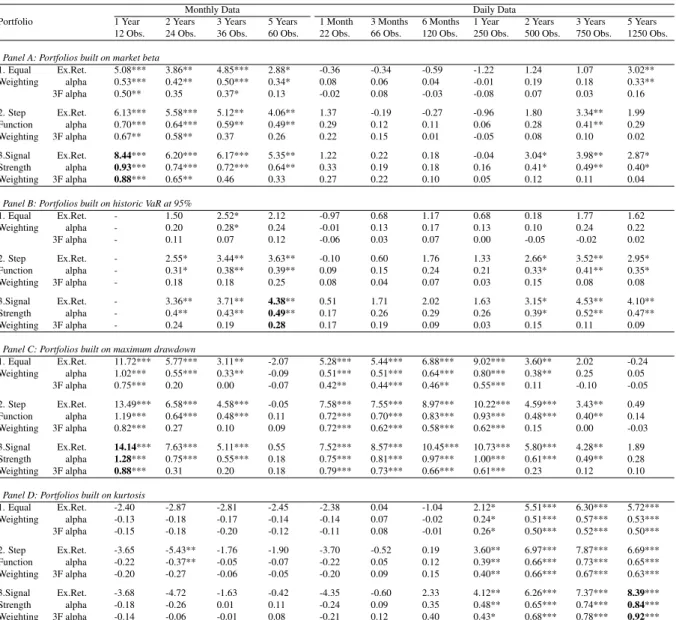
In this part, strategies are tested on their robustness with regards to the length of the risk es-timation window and the way assets are weighted within the long and the short portfolio. As idiosyncratic volatility strategies have not shown to be significant in the previous tests, the focus is now only on rankings based on market beta, Value at Risk at 95 percent confidence, maximum drawdown and excess kurtosis. Table 3 contains grids for each ranking variable with signifi-cant values labelled with stars. Excess returns are in percent per year, alphas are in percent per month. Portfolios are formed with the three weighting methods explained in section 3. Risk estimators are based on variously lengthy windows in both daily and monthly data.
Even though showing up in the previous tests, the market beta-based strategies do not work consistently in daily data. However, there is a large cluster of significant strategies when risks are estimated on monthly data, especially when taking into account the information contained in the absolute and relative level of the beta estimator for the portfolio composition. The most profitable strategy on both an absolute and a risk-adjusted basis is built upon 1 year of monthly observations and weighted according to Equations (4) and (5). Given the fact that the strategy yields significant positive returns irrespective of portfolio weighting and longer estimation win-dows, it appears rather robust. On the other hand, when using the same window lengths of daily data, none of the findings persists.
Moving to the historic VaR@95%-strategies, it appears they gain traction when using longer formation periods. This is intuitive as this measure of risk becomes more meaningful the more data points are available. The best results in-sample are achieved when using 5 years of monthly data and again the weighting method that considers the strength of the ranking signal. The strategy has a positive annual excess return of 4.38 percent and a positive simple alpha of 0.49 percent, both of which are significant at the 95 percent confidence level. However, none of the portfolios based on Value at Risk significantly outperforms when adjusting for three risk factors.
When considering rankings based on maximum drawdown, it seems likely that strategies overlap with momentum strategies as the strategy penalises assets with poor past performance. A wide range of combinations of risk estimation parameters and portfolio composition methods
Table 3: A closer look at robustness with regards to formation windows and asset weighting scheme
Monthly Data Daily Data
Portfolio 1 Year 2 Years 3 Years 5 Years 1 Month 3 Months 6 Months 1 Year 2 Years 3 Years 5 Years 12 Obs. 24 Obs. 36 Obs. 60 Obs. 22 Obs. 66 Obs. 120 Obs. 250 Obs. 500 Obs. 750 Obs. 1250 Obs. Panel A: Portfolios built on market beta
1. Equal Ex.Ret. 5.08*** 3.86** 4.85*** 2.88* -0.36 -0.34 -0.59 -1.22 1.24 1.07 3.02** Weighting alpha 0.53*** 0.42** 0.50*** 0.34* 0.08 0.06 0.04 -0.01 0.19 0.18 0.33** 3F alpha 0.50** 0.35 0.37* 0.13 -0.02 0.08 -0.03 -0.08 0.07 0.03 0.16 2. Step Ex.Ret. 6.13*** 5.58*** 5.12** 4.06** 1.37 -0.19 -0.27 -0.96 1.80 3.34** 1.99 Function alpha 0.70*** 0.64*** 0.59** 0.49** 0.29 0.12 0.11 0.06 0.28 0.41** 0.29 Weighting 3F alpha 0.67** 0.58** 0.37 0.26 0.22 0.15 0.01 -0.05 0.08 0.10 0.02 3.Signal Ex.Ret. 8.44*** 6.20*** 6.17*** 5.35** 1.22 0.22 0.18 -0.04 3.04* 3.98** 2.87* Strength alpha 0.93*** 0.74*** 0.72*** 0.64** 0.33 0.19 0.18 0.16 0.41* 0.49** 0.40* Weighting 3F alpha 0.88*** 0.65** 0.46 0.33 0.27 0.22 0.10 0.05 0.12 0.11 0.04
Panel B: Portfolios built on historic VaR at 95%
1. Equal Ex.Ret. - 1.50 2.52* 2.12 -0.97 0.68 1.17 0.68 0.18 1.77 1.62 Weighting alpha - 0.20 0.28* 0.24 -0.01 0.13 0.17 0.13 0.10 0.24 0.22 3F alpha - 0.11 0.07 0.12 -0.06 0.03 0.07 0.00 -0.05 -0.02 0.02 2. Step Ex.Ret. - 2.55* 3.44** 3.63** -0.10 0.60 1.76 1.33 2.66* 3.52** 2.95* Function alpha - 0.31* 0.38** 0.39** 0.09 0.15 0.24 0.21 0.33* 0.41** 0.35* Weighting 3F alpha - 0.18 0.18 0.25 0.08 0.04 0.07 0.03 0.15 0.08 0.08 3.Signal Ex.Ret. - 3.36** 3.71** 4.38** 0.51 1.71 2.02 1.63 3.15* 4.53** 4.10** Strength alpha - 0.4** 0.43** 0.49** 0.17 0.26 0.29 0.26 0.39* 0.52** 0.47** Weighting 3F alpha - 0.24 0.19 0.28 0.17 0.19 0.09 0.03 0.15 0.11 0.09
Panel C: Portfolios built on maximum drawdown
1. Equal Ex.Ret. 11.72*** 5.77*** 3.11** -2.07 5.28*** 5.44*** 6.88*** 9.02*** 3.60** 2.02 -0.24 Weighting alpha 1.02*** 0.55*** 0.33** -0.09 0.51*** 0.51*** 0.64*** 0.80*** 0.38** 0.25 0.05 3F alpha 0.75*** 0.20 0.00 -0.07 0.42** 0.44*** 0.46** 0.55*** 0.11 -0.10 -0.05 2. Step Ex.Ret. 13.49*** 6.58*** 4.58*** -0.05 7.58*** 7.55*** 8.97*** 10.22*** 4.59*** 3.43** 0.49 Function alpha 1.19*** 0.64*** 0.48*** 0.11 0.72*** 0.70*** 0.83*** 0.93*** 0.48*** 0.40** 0.14 Weighting 3F alpha 0.82*** 0.27 0.10 0.09 0.72*** 0.62*** 0.58*** 0.62*** 0.15 0.00 -0.03 3.Signal Ex.Ret. 14.14*** 7.63*** 5.11*** 0.55 7.52*** 8.57*** 10.45*** 10.73*** 5.80*** 4.28** 1.89 Strength alpha 1.28*** 0.75*** 0.55*** 0.18 0.75*** 0.81*** 0.97*** 1.00*** 0.61*** 0.49** 0.28 Weighting 3F alpha 0.88*** 0.31 0.20 0.18 0.79*** 0.73*** 0.66*** 0.61*** 0.23 0.12 0.10
Panel D: Portfolios built on kurtosis
1. Equal Ex.Ret. -2.40 -2.87 -2.81 -2.45 -2.38 0.04 -1.04 2.12* 5.51*** 6.30*** 5.72*** Weighting alpha -0.13 -0.18 -0.17 -0.14 -0.14 0.07 -0.02 0.24* 0.51*** 0.57*** 0.53*** 3F alpha -0.15 -0.18 -0.20 -0.12 -0.11 0.08 -0.01 0.26* 0.50*** 0.52*** 0.50*** 2. Step Ex.Ret. -3.65 -5.43** -1.76 -1.90 -3.70 -0.52 0.19 3.60** 6.97*** 7.87*** 6.69*** Function alpha -0.22 -0.37** -0.05 -0.07 -0.22 0.05 0.12 0.39** 0.66*** 0.73*** 0.65*** Weighting 3F alpha -0.20 -0.27 -0.06 -0.05 -0.20 0.09 0.15 0.40** 0.66*** 0.67*** 0.63*** 3.Signal Ex.Ret. -3.68 -4.72 -1.63 -0.42 -4.35 -0.60 2.33 4.12** 6.26*** 7.37*** 8.39*** Strength alpha -0.18 -0.26 0.01 0.11 -0.24 0.09 0.35 0.48** 0.65*** 0.74*** 0.84*** Weighting 3F alpha -0.14 -0.06 -0.01 0.08 -0.21 0.12 0.40 0.43* 0.68*** 0.78*** 0.92***
Annualised excess returns, monthly commodity CAPM alphas and monthly 3-Factor alphas in percent for strategies using different risk estimation and portfolio weighting methods. 1. Equal Weighting corresponds to Equation (2), 2. Step Function Weighting corresponds to Equation (3), and 3. Signal Strength Weighting corresponds to Equations (4) and (5). * marks values significant at 90 percent, ** marks values significant at 95 percent, and *** marks values significant at 99 percent. The bold strategies are used in further analysis as the third weighting method consistently improves results over the other methods, and the chosen estimation periods appear to most appropriately capture the respective risk estimators irrespective of weighting method.
indeed result in substantial positive returns. 26 of the 33 strategies displayed in Table 3 have significant positive alphas with regards to the equally weighted index. It is striking that suc-cessful strategies are clustered in the shorter estimation windows in monthly data as well as in daily data. The most compelling results are achieved in windows of one year of data, a time
frame which is commonly chosen for momentum strategies6. When also considering the value
and momentum in commodities factors of Asness et al. (2013b), 15 of the strategies still have significant positive abnormal returns. Contrary to the prediction of the effect disappearing when
6The momentum factor used in the 3-factor model is formed based on a window of 12 months while skipping
accounting for momentum, the large number of unaffected strategies indicates the existence of a distinguishable underlying return pattern.
At last, the kurtosis-based strategies work well when having a data window with many observations irrespective of the portfolio composition method. This makes sense, as a larger sample is more likely to contain extreme values that help to improve the quality of the kurtosis estimator. Hence, portfolios are insignificant in monthly data and start to show significance in daily data when 250 observations are included in the estimation. Most profitable is a strat-egy that combines a formation period of five years with weights following the signal strength method. Different ways of asset weighting and shorter windows of down to two years are equally significant and hint towards robustness of the kurtosis strategy.
The four tested approaches, buying low-beta commodities and shorting high-beta
commodi-ties, buying commodities with a high (less negative) VaR7and shorting commodities with a low
VaR (more negative), buying commodities with less negative drawdowns and shorting
com-modities with more negative drawdowns8, and buying high-kurtosis commodities and selling
low-kurtosis commodities, all display some significant returns. However, the evidence on the Value at Risk method remains thin and no significant abnormal return can be proven for that block of strategies when adjusting for more than one factor. The remaining three approaches all show some robustness in proximity of the parameters they work best in. While beta- and VaR-based strategies are in line with previous literature on low-risk investing, the findings on kurtosis is opposed to the concept of a low-risk return premium as it buys assets with leptokur-tic return distributions and vice versa. These are commonly considered risky because extreme events (”fat tails”) occur in higher frequency.
4.3
Investability
So far, the analysis has focused on demonstrating the existence of a low-risk return premium in commodity futures markets. The following parts will investigate more the riskiness of the investment strategies and the implementability as such.
7Negative by definition. Therefore, buying commodities with a high VaR means buying low-risk commodities. 8Again, maximum drawdown is defined negatively. Hence, this strategy is a low-risk investment style.
4.3.1 Risks of Low-Risk Investing
Correlations When investing in a long-short strategy, the goal is to achieve uncorrelated
re-turns to common aggregates. Therefore, for a strategy to be attractive for an actual investment, monitoring correlations with market indices and acknowledged return factors is crucial. It is further interesting to review how strategies relate to each other. Table 4 shows return corre-lations of selected strategies amongst them and with the return factors used in the commodity pricing models used in this research. Additionally, the correlation with the market excess return on equities is recorded.
The selected strategies that have shown significant in previous tests do not appear to be much interrelated. The highest correlation is between the market beta strategy and the maximum drawdown strategy with 0.23. This indicates some similar asset choices of the two strategies, but there are still considerable differences between the two. When looking at the relations towards return factors in the commodities markets, there is a slight relation of the market beta strategy with the market factor of 0.25. Nevertheless, this is not surprising as the strategy carries a beta loading over the full sample of 0.49. In line with the hypothesis of the drawdown-based strategy being connected to the momentum premium, the correlation between the two is 0.46. This indicates a strong overlap and weakens the case for the existence of a low-risk return premium in commodity markets when looking at this strategy only. At the same time, there is a negative correlation of -0.21 with the value premium, which is another similarity with the momentum factor (see Asness et al. (2013b)). The third strategy (the kurtosis-based portfolio) does not seem related to any of the factors in commodities with correlations being close to zero. None of the strategies appears to be related to the equities markets.
Table 4: Correlations of 3 selected strategies with each other and with return factors in com-modities and equities
Strategies Commodity Factors Equity Factor
Strategy 1 Strategy 2 Strategy 3 Market Value Momentum Market
Strategy 1: Market Beta 1.0000 0.2272 0.0560 0.2538 0.0430 -0.0451 0.0310
Strategy 2: Maximum Drawdown 0.2272 1.0000 0.0718 0.0742 -0.2132 0.4629 -0.0095
Strategy 3: Kurtosis 0.0560 0.0718 1.0000 0.0899 -0.0908 0.0145 -0.0501
The table shows correlations of the return time series. Strategy 1 is formed by ranking on market beta estimated over windows of 1 year of monthly data and portfolio weights according to the signal strength method. Strategy 2 is formed by ranking on maximum drawdown estimated over windows of 1 year of monthly data and portfolio weights according to the signal strength method. Strategy 3 is formed by ranking on kurtosis estimated over windows of 5 years of daily data and portfolio weights according to the signal strength method. Market factors are in excess of the risk-free rate. The commodity market factor is an equally weighted index of all assets. Value and momentum factors are from Asness et al. (2013b).
Drawdowns One of the main concerns when implementing a strategy is to make big losses over a prolonged period of time. Looking at backtests of the three strategies as indexes starting at a value of 100 in Figure 1, their good overall performance is apparent. With the equally weighted market index as benchmark in Figure 1d, overlaps can be observed. Considering the plots alone, the three strategies seem to be levered versions of the index. However, the previous part has shown that this is not the case as correlations are negligible. In terms of drawdown, the market index suffered its biggest losses of 51.89 percent from January 1990 to July 1996.
The market beta strategy as depicted in Figure 1a has a prolonged drawdown period from Mai 1990 to April 1999, where the portfolio loses 60.06 percent of value. Despite an interim recovery, it takes until September 2004 for the strategy to reach its previous hight. Even though this does not coincide with the index drawdown period and the strategy gains 6.21 percent during the market’s biggest losing streak, a period of losses that severe and that long makes the ’Betting against Beta’-strategy unattractive for implementation.
Figure 1: Index plots of the systematic strategies and drawdown periods
1960 1965 1970 1975 1980 1985 1990 1995 2000 2005 2010 2015 2000 4000 6000 8000 10000 12000 Mai 1990 April 1999 -60.06%
(a) Strategy 1: Market beta
1960 1965 1970 1975 1980 1985 1990 1995 2000 2005 2010 2015 2 4 6 8 10 12 14 16 #104 September 1982 Mai 1983 -45.45%
(b) Strategy 2: Maximum drawdown
1960 1965 1970 1975 1980 1985 1990 1995 2000 2005 2010 2015 1000 2000 3000 4000 5000 6000 7000 November 1967 December 1976 -67.65% (c) Strategy 3: Kurtosis 1960 1965 1970 1975 1980 1985 1990 1995 2000 2005 2010 2015 200 400 600 800 1000 1200 1400 January 1980 July 1986 -51.89%
Turning to the maximum drawdown ranked strategy in Figure 1b, a far shorter period of losses occurs from September 1982 until Mai 1983. During those eight months the portfolio forfeits 45.45 percent. This lays inside the maximum drawdown period of the commodity fu-tures market. However, during this whole bearish period of six and a half years, the strategy gains 19.36 percent. The overall steady performance is underlined by a percentage of positive months in the whole sample of 61.37 percent.
The third strategy’s backtest performance is displayed in Figure 1c. Its overall good per-formance is overshadowed by heavy losses of 67.65 percent near the beginning of the sample from November 1967 to December 1976. Even though the market back then with only a few as-sets may have been fundamentally different from the conditions nowadays, this drought of nine years clouds the strategy’s attractiveness and it took the portfolio almost three years to make up for the losses. On the other hand, during the market drawdown, the strategy wins 14.36 percent, effectively offering diversification to the market portfolio.
4.3.2 Transaction Volume
A common pitfall for the investment into systematic return premiums is that they involve a high turnover of positions. When trying to span all the information and diversification potential of all assets available, the frequent readjustment of the portfolio becomes very costly. Further,
considering all assets requires a large total investment9due to minimum contract sizes. To ease
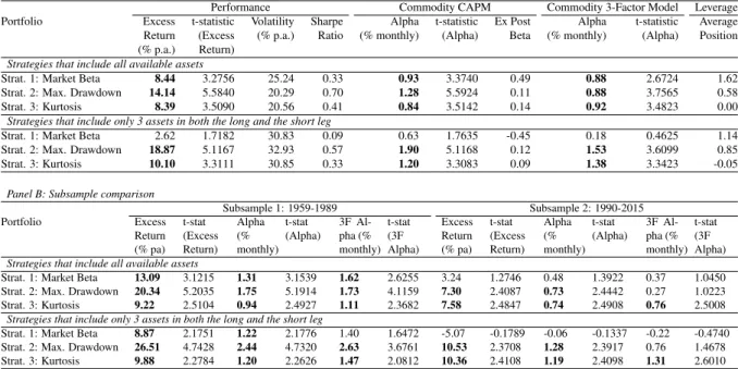
these boundaries, portfolios that only include three assets on both the long and the short side are scrutinised in Table 5.
As reducing the number of assets is equivalent with reducing diversification, risks are more concentrated and the idiosyncratic component has a stronger influence. Panel A of Table 5 shows that volatilities of all three strategies climb to over 30 percent per year. Even though the maximum drawdown strategy and the kurtosis strategy achieve higher annual excess returns, reducing position count leads to lower risk-adjusted performance when looking at Sharpe Ratio. However, alphas over the commodity CAPM and the 3-Factor model show a different picture. Here, lowering the number of assets significantly enhances outperformance. The only strategy
Table 5: Absolute and risk-adjusted performance of all-asset and 3-asset portfolios in the full sample and in subsamples
Panel A: Full-sample comparison
Performance Commodity CAPM Commodity 3-Factor Model Leverage
Portfolio Excess t-statistic Volatility Sharpe Alpha t-statistic Ex Post Alpha t-statistic Average
Return (Excess (% p.a.) Ratio (% monthly) (Alpha) Beta (% monthly) (Alpha) Position
(% p.a.) Return)
Strategies that include all available assets
Strat. 1: Market Beta 8.44 3.2756 25.24 0.33 0.93 3.3740 0.49 0.88 2.6724 1.62
Strat. 2: Max. Drawdown 14.14 5.5840 20.29 0.70 1.28 5.5924 0.11 0.88 3.7565 0.58
Strat. 3: Kurtosis 8.39 3.5090 20.56 0.41 0.84 3.5142 0.14 0.92 3.4823 0.00
Strategies that include only 3 assets in both the long and the short leg
Strat. 1: Market Beta 2.62 1.7182 30.83 0.09 0.63 1.7635 -0.45 0.18 0.4625 1.14
Strat. 2: Max. Drawdown 18.87 5.1167 32.93 0.57 1.90 5.1168 0.12 1.53 3.6099 0.85
Strat. 3: Kurtosis 10.10 3.3111 30.85 0.33 1.20 3.3083 0.09 1.38 3.3423 -0.05
Panel B: Subsample comparison
Subsample 1: 1959-1989 Subsample 2: 1990-2015 Portfolio Excess Return (% pa) t-stat (Excess Return) Alpha (% monthly) t-stat (Alpha) 3F Al-pha (% monthly) t-stat (3F Alpha) Excess Return (% pa) t-stat (Excess Return) Alpha (% monthly) t-stat (Alpha) 3F Al-pha (% monthly) t-stat (3F Alpha) Strategies that include all available assets
Strat. 1: Market Beta 13.09 3.1215 1.31 3.1539 1.62 2.6255 3.24 1.2746 0.48 1.3922 0.37 1.0450
Strat. 2: Max. Drawdown 20.34 5.2035 1.75 5.1914 1.73 4.1159 7.30 2.4087 0.73 2.4442 0.27 1.0223
Strat. 3: Kurtosis 9.22 2.5104 0.94 2.4927 1.11 2.3682 7.58 2.4847 0.74 2.4908 0.76 2.5008
Strategies that include only 3 assets in both the long and the short leg
Strat. 1: Market Beta 8.87 2.1751 1.22 2.1776 1.40 1.6472 -5.07 -0.1789 -0.06 -0.1337 -0.22 -0.4740
Strat. 2: Max. Drawdown 26.51 4.7428 2.44 4.7320 2.63 3.6761 10.53 2.3708 1.28 2.3917 0.76 1.4678
Strat. 3: Kurtosis 9.88 2.2784 1.20 2.2626 1.47 2.0812 10.36 2.4108 1.19 2.4098 1.31 2.6010
Strategy 1 is formed by ranking on market beta estimated over windows of 1 year of monthly data. Strategy 2 is formed by ranking on maximum drawdown estimated over windows of 1 year of monthly data. Strategy 3 is formed by ranking on kurtosis estimated over windows of 5 years of daily data. All portfolio weights are according to the signal strength method as in Equations (4) and (5). Subsamples are split at the first day of 1990. The three factor model can only be estimated starting in 1972 when all three factors are available.
falling insignificant in our sample is the market beta-based portfolio. Also striking is that the market-beta strategy requires most leverage to hedge ex ante beta exposure. Nevertheless, it carries the highest systematic risk in the form of ex post market beta.
Looking at the two subsamples in Panel B of Table 5, it becomes clear that almost all effects have weakened in the more recent period. While the low-beta effect has become unrecognis-able and even makes losses from 1990 when only including three assets, the other two strategies remain significant at the 95 percent confidence level. What is more, both show abnormal re-turns over the commodity CAPM and the kurtosis strategy even significantly outperforms the 3-Factor model. This does not change and even grows stronger when constructing a leaner portfolio. Another observation is that the drawdown strategy is absorbed by the value and mo-mentum factor from 1990 as the 3-Factor model explains returns in the second subsample and the strategy’s abnormal returns fall insignificant.
5
Conclusion
Classic factor-based asset-pricing models have shown shortcomings in explaining the pricing of systematic risk in the form of beta in most asset classes. This research shows that also in the commodities futures markets, risk-based factors can be constructed that yield significantly pos-itive excess returns. Further, adjusting for common asset class-specific systematic return factors does not fully take away the effects. Specifically, strategies based on market beta, maximum drawdown and historic excess kurtosis prove significant and show some robustness towards parameter choice.
The fact that the ’Betting against Beta’-factor shows the weakest and least persistent ev-idence of the three is in line with its most wide-spread explanation, leverage constraints or
leverage-aversion10. In an asset class that is leveraged by definition, this reasoning only has
weak implications. It is thinkable however, that both hedgers and speculators predominantly crowd into the contracts that are perceived most risky, leading to relative overpricing. The sec-ond demonstrated effect based on maximum drawdown is partly explained by the momentum effect. With a correlation of almost 0.5, a considerable share of the abnormal returns is taken away when adjusting for that factor. Especially in the more recent market environment after 1990, the effect is consumed by the momentum factor of the same asset class (see Asness et al. (2013b) in commodities). The third finding, the significance of the high-kurtosis effect in this market, is in line with the conventional relation of risk and return where higher risk is intu-itively rewarded with higher return (Cremers et al. (2015) report the same relation jump risk and returns in equity futures options). Though not yielding excess returns as high as the other found factors, this effect consistently shows up significant throughout subsamples and portfolio modifications.
To concludingly answer the question whether the low-risk anomaly also exists in commod-ity markets, it is necessary to also consider the limitations of this research. Given the nature of the futures market, tests can only be conducted on a comparatively small number of assets. Ad-ditionally, the capabilities to perform out-of-sample tests are limited. With commodities being traded globally, there are no geographical distinctions to be made. Besides, dividing assets into
groups would result in even smaller width of data and sabotage the meaningfulness of results. Another limitation is related to the choice of estimation and portfolio composition parameters. Reproducing the approaches of previous literature, it becomes clear that this involves several non-trivial choices with regards to data frequency, estimation period, asset weighting and hedg-ing. All these can radically alter the results and change deducted inference. The reported results in this research have been shown to exist in different settings of parameters. Nevertheless, given the number of possible combinations of parameter choices, doubts remain on whether the shown systematic effects are not just statistical flaws (type I errors).
Considering the shown evidence, it is definitely possible to construct significant low-risk factors in the commodities futures markets. Deviations from previous papers’ choice of estima-tion period make the difference towards a significant ’Betting against Beta’-factor. To further explore this result, it would be interesting to apply the same parameters in futures markets on different underlyings and compare eventual outcomes to the literature. Yet another impulse towards further exploration is released by the findings on kurtosis-based portfolios. Given the dependency of kurtosis estimators on a sufficient quantity of observations, especially data in higher frequency could lead to additional insights. Moreover, it would be informative to survey results from other futures classes and explore how tail risks are compensated in that class.
6
Appendix A: Data Summary Statistics
Table 6: Descriptive statistics of the return time series of the commodities futures and the return factors used in the analysis
Panel A: Commodity Futures
Commodity Class First Last Number of Number of Return Volatility Observation Observation Daily Monthly (% p.a.) (% p.a.)
Observations Observations
Crude Oil Energy 1983/03/31 2015/02/27 8,006 382 3.96 33.12 Gasoline Energy 1984/12/04 2015/02/27 7,579 361 10.57 32.17 Heating Oil Energy 1979/03/07 2015/02/27 9,023 430 4.00 29.99 Natural Gas Energy 1990/04/04 2015/02/27 6,246 297 -17.22 45.31 Gas-Oil-Petroleum Energy 1986/06/04 2015/02/27 7,127 343 7.32 29.89 Propane Energy 1987/08/24 2007/10/31 5,035 241 19.20 29.81 Coffee Agriculture 1972/08/17 2015/02/27 10,635 509 -0.74 33.48 Rough Rice Agriculture 1986/08/21 2015/02/27 7,180 340 -7.37 22.79 Orange Juice Agriculture 1967/02/02 2015/02/27 12,026 575 0.00 27.59 Sugar Agriculture 1961/01/05 2015/02/27 13,502 648 -2.85 38.12 Cocoa Agriculture 1959/07/02 2015/02/27 13,897 666 -1.36 28.48 Milk Agriculture 1997/08/07 2015/02/27 4,415 209 2.48 21.60 Soybean Oil Agriculture 1959/07/02 2015/02/27 14,006 666 1.94 24.78 Soybean Meal Agriculture 1959/07/06 2015/02/27 14,004 666 6.07 24.98 Soybeans Agriculture 1959/07/02 2015/02/27 14,002 666 2.52 21.72 Corn Agriculture 1959/07/02 2015/02/27 14,008 666 -4.28 21.28 Oats Agriculture 1959/07/02 2015/02/27 14,003 666 -4.04 26.20 Wheat Agriculture 1959/07/02 2015/02/27 13,997 666 -4.24 23.80 Canola Agriculture 1977/04/12 2015/02/27 9,243 451 -3.21 20.51 Barley Agriculture 1989/05/25 2012/08/09 5,703 271 -3.05 20.71 Cotton Metals/Fibers 1959/07/02 2015/02/27 13,914 666 -0.72 21.63 Gold Metals/Fibers 1975/01/02 2015/02/27 10,088 481 -0.60 19.43 Silver Metals/Fibers 1963/06/14 2015/02/27 12,948 619 -1.06 28.48 Copper Metals/Fibers 1959/07/02 2015/02/27 13,930 666 7.83 25.49 Lumber Metals/Fibers 1969/10/02 2015/02/27 11,439 543 -7.58 25.85 Palladium Metals/Fibers 1977/01/06 2015/02/27 9,545 456 6.58 31.55 Platinum Metals/Fibers 1969/01/03 2015/02/27 11,571 552 0.97 25.78 Rubber Metals/Fibers 1992/01/07 2015/02/27 5,491 276 -2.86 32.93 Feeder Cattle Livestock 1971/12/01 2015/02/27 10,847 518 2.76 15.20 Live Cattle Livestock 1964/12/01 2015/02/27 12,648 602 3.80 15.38 Lean Hogs Livestock 1966/03/01 2015/02/27 12,337 587 0.77 23.28 Pork Bellies Livestock 1961/09/19 2010/06/30 12,164 578 -3.44 30.47
Panel B: Risk Factors
Factor First Last Number of Number of Return Volatility Observation Observation Daily Monthly (% p.a.) (% p.a.)
Observations Observations
Equity: Market Excess 1959/07/01 2015/02/27 13,987 667 4.97 15.42 Equity: Size 1959/07/01 2015/02/27 13,987 667 1.27 8.09 Equity: Value 1959/07/01 2015/02/27 13,987 667 4.12 7.65 Equity: Momentum 1959/07/01 2015/02/27 13,987 667 7.81 10.75 Commodities: Market Equal Index 1959/07/01 2015/02/27 14,019 666 3.70 11.04 Commodities: Value 1972/01 2015/01 0 517 3.68 22.89 Commodities: Momentum 1972/01 2015/01 0 517 9.44 21.67
7
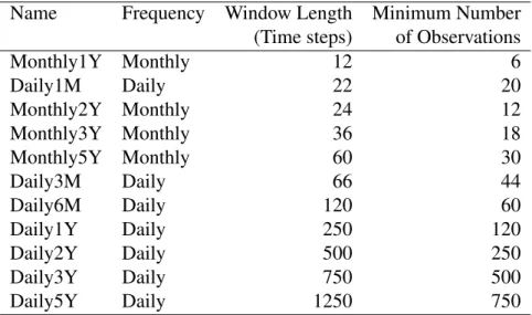
Appendix B: Details of Risk Estimation
Table 7: Parameters of the risk estimation windows
Name Frequency Window Length Minimum Number
(Time steps) of Observations
Monthly1Y Monthly 12 6 Daily1M Daily 22 20 Monthly2Y Monthly 24 12 Monthly3Y Monthly 36 18 Monthly5Y Monthly 60 30 Daily3M Daily 66 44 Daily6M Daily 120 60 Daily1Y Daily 250 120 Daily2Y Daily 500 250 Daily3Y Daily 750 500 Daily5Y Daily 1250 750
If the window contains less observations than the minimum number, the asset is excluded from the portfolio in that period.
References
Yakov Amihud. Illiquidity and stock returns: Cross-section and time-series effects. Journal of Financial Markets, 5(1):31–56, 2002.
Andrew Ang, Robert J Hodrick, Yuhang Xing, and Xiaoyan Zhang. The cross-section of volatil-ity and expected returns. The Journal of Finance, 61(1):259–299, 2006.
C Asness, A Ilmanen, R Israel, and T Moskowitz. Investing with style. Journal of Investment Management, forthcoming, 2013a.
Clifford S Asness, Tobias J Moskowitz, and Lasse Heje Pedersen. Value and momentum every-where. The Journal of Finance, 68(3):929–985, 2013b.
Malcolm Baker, Brendan Bradley, and Jeffrey Wurgler. Benchmarks as limits to arbitrage: Understanding the low-volatility anomaly. Financial Analysts Journal, 67(1):40–54, 2011. Turan G Bali and Nusret Cakici. Idiosyncratic volatility and the cross section of expected
Nicholas Barberis and Andrei Shleifer. Style investing. Journal of financial Economics, 68(2): 161–199, 2003.
David Blitz and Pim Van Vliet. The volatility effect: Lower risk without lower return. Journal of Portfolio Management, pages 102–113, 2007.
David Blitz, Eric G Falkenstein, and Pim Van Vliet. Explanations for the volatility effect: An overview based on the capm assumptions. Available at SSRN 2270973, 2013.
Martijn Boons and Melissa Porras Prado. Momentum signals in the term structure of commodity futures. Available at SSRN, 2015.
Mark Carhart, Ui-Wing Cheah, Giorgio De Santis, Harry Farrell, and Robert Litterman. Exotic beta revisited. Financial Analysts Journal, 70(5):24–52, 2014.
Mark M Carhart. On persistence in mutual fund performance. The Journal of Finance, 52(1): 57–82, 1997.
Bo Young Chang, Peter Christoffersen, and Kris Jacobs. Market skewness risk and the cross section of stock returns. Journal of Financial Economics, 107(1):46–68, 2013.
Martijn Cremers, Michael Halling, and David Weinbaum. Aggregate jump and volatility risk in the cross-section of stock returns. The Journal of Finance, 70(2):577–614, 2015.
Eugene F Fama and Kenneth R French. The cross-section of expected stock returns. The Journal of Finance, 47(2):427–465, 1992.
Eugene F Fama and Kenneth R French. Common risk factors in the returns on stocks and bonds. Journal of Financial Economics, 33(1):3–56, 1993.
Eugene F Fama and Kenneth R French. A five-factor asset pricing model. Journal of Financial Economics, 116(1):1–22, 2015.
Andrea Frazzini and Lasse Heje Pedersen. Betting against beta. Journal of Financial Eco-nomics, 111(1):1–25, 2014.
Fangjian Fu. Idiosyncratic risk and the cross-section of expected stock returns. Journal of Financial Economics, 91(1):24–37, 2009.
Campbell R Harvey, Yan Liu, and Heqing Zhu. ... and the cross-section of expected returns. Review of Financial Studies, page hhv059, 2015.
Ron Israel and Thomas Maloney. Understanding style premia. Journal of Investing, 23(4): 15–22, 2014.
Narasimhan Jegadeesh and Sheridan Titman. Returns to buying winners and selling losers: Implications for stock market efficiency. The Journal of Finance, 48(1):65–91, 1993.
Michael C Jensen, Fischer Black, and Myron S Scholes. The capital asset pricing model: Some empirical tests. 1972.
Ralph SJ Koijen, Tobias J Moskowitz, Lasse Heje Pedersen, and Evert B Vrugt. Carry. Techni-cal report, National Bureau of Economic Research, 2013.
Robert B Litterman. Beyond active alpha. In CFA Institute Conference Proceedings Quarterly, volume 25, pages 14–21. CFA Institute, 2008.
R David McLean and Jeffrey Pontiff. Does academic research destroy stock return predictabil-ity? The Journal of Finance, 71(1):5–32, 2016.
Tobias J Moskowitz, Yao Hua Ooi, and Lasse Heje Pedersen. Time series momentum. Journal of Financial Economics, 104(2):228–250, 2012.
Robert Novy-Marx. The other side of value: The gross profitability premium. Journal of Financial Economics, 108(1):1–28, 2013.
Lubos Pastor and Robert F Stambaugh. Liquidity risk and expected stock returns. Technical report, National Bureau of Economic Research, 2001.
Ronnie Sadka. Momentum and post-earnings-announcement drift anomalies: The role of liq-uidity risk. Journal of Financial Economics, 80(2):309–349, 2006.
William F Sharpe. Capital asset prices: A theory of market equilibrium under conditions of risk. The Journal of Finance, 19(3):425–442, 1964.
Sheridan Titman, KC John Wei, and Feixue Xie. Capital investments and stock returns. Journal of Financial and Quantitative Analysis, 39(04):677–700, 2004.