A Work Project, presented as part of the requirements for the Award of a Master’s Degree in Finance from the NOVA – School of Business and Economics.
The role of dispersion into assets allocation
Edoardo Colella - 912
A Project carried out on the Hedge Fund course, under the supervision of: Pedro Lameira
The role of dispersion into assets allocation
Abstract
Dispersion of returns has gained a lot of attention as a measure to distinguish good and bad investment opportunities time. In the following dissertation, the cross-sectional returns volatility is analyzed over a fifteen year period across the S&P100 Index composition. The main inference drawn from the data sample is that the canonical measure of dispersion is highly macro-risk driven and therefore more biased towards returns volatility rather than its correlation component.
Purpose of the project
In both the finance and economics world there has been an increasing interest in the study of the cross-asset correlation role in portfolio management. The association of correlation with the precept of diversification has been dominant in both theory and practice since and before the formal publication of the CAPM by William Sharpe in the 1964. Regardless of the high number of attempts to manage correlation for protection purposes, many are the events that is easy to think about where huge losses were prompt by stocks -but more broadly any assets- moving down in unison. Financial crises are the most suitable example to recall. They do prove that, mostly for any type of investor, diversification shrinks when you need it the most. This concept has been crucial and represents the origination of my work project. My init ia l and actual purpose is to deepen the study of the assets’ behavior, to enhance investors’ skillset in managing their portfolio during bad times -namely when volatility and correlation spike-.
bad time scenarios, being likewise important in active portfolio management. In the latter, a reasonable degree of dispersion is in fact required to create the right opportunity set for any manger to succeed. Beyond the ability of over and under-weighting good and bad performers, active portfolio management would be meaningless without assets prices’ divergences. The return dispersion is associated with the cross-sectional standard deviation of returns, and mathematically it is formulated by the following expression:
𝜎 ∗ √1 − 𝜌1
It follows intuitively that dispersion is positively related to standard deviation and negative ly to correlation. Dispersion is the ultimate tool of my dissertation, since it captures the correlation effect and it looks like a useful proxy to distinguish good periods -high dispersion- from bad and challenging opportunity times -low dispersion-. The following study is dividable in two parts, for which similar methods are applied to analyze different periods of time series stocks’ returns. In the first one, I observe returns’ correlations and dispersions over 15 years, applying and calibrating the tools I will further employ. The second one is dedicated to the implementation of an investment strategy that relies on the former findings and methods. The hypothesis here tested aims at verifying whether periods of high and low dispersion are strictly related to, respectively, high and low degree of profitability.
1.The role of cross-sectional dispersion in active portfolio management. Larry R. Gorman, Steven G. Sapra,
Literature review
Literature-wise, assets returns’ dispersion has gained a high degree of attention from the academic world. Studies and researches range in a wide interval covering aspects from its predictive power to its implementation in relative value portfolio strategies. Paulo Maio2 (2015) analyzes the return dispersion for forecasting the equity premium. He compares the predictive returns’ dispersion power against a series of well-known predictors such as dividend-to-price ratio, earnings-to-price ratio and many others. His main finding shows that equity premium reductions are consistently forecasted by a decrease in return dispersion. Gorman, Sapra and Weigand3 (2010) derive the Modern Portfolio theory using dispersion as a measure of risk rather than market volatility. They focus on the relationship between portfolio risk metrics and dispersion, showing how the latter is positively related with both idiosyncratic and systemic risk and primary impacting on the idiosyncratic component. The same authors (2010)4 extend their dispersion study into relative values portfolio, comb ing the aforementioned predictive power with the VIX index to forecast alpha distribution. In their first work, they conclude that higher dispersion does favor absolute return investors over benchmarked portfolio managers. In fact, in their second paper they aim at improving absolute return investment strategies combining signal arising from dispersion and the implied volatility index. Many other authors have dealt with the relationship between returns dispersion and stock market volatility (Harvey and Strivers, 2003), or including it within a
2 Cross-sectional return dispersion and the equity premium. Paulo Maio. 2015.
3 The role of cross-sectional dispersion in active portfolio management. Larry R. Gorman, Steven G. Sapra, Robert A. Weigand. 2010.
momentum strategy (Bhootra, 2011). Applications of return dispersion have not only involved financial markets studies. Loungani, Rush and Tave (1990) consider cross-sectional returns volatility implications on the unemployment rate. Pashtan, Kostin, Sneider, Snider, Menon5 and Sanchez derive a proxy for dispersion returns that is central in the second part of the following dissertation, introducing the concept of dispersion score. This paper is intended to proceed the study of dispersion as a tool to foresee bad times and at the same time as a signal for guiding investors’ allocation decisions.
Discussion of the topic- Hypothesis Testing
Return dispersion is defined as the cross sectional volatility of stock returns. It gauges the extent to which stocks’ prices move in different directions. The measurement showed in the first section represents the dispersion form under the VCV assumptions6. In the following dissertation, two measures of returns dispersion will be employed. The one showed previously will be referred to as the ordinary, canonical or full dispersion. The second estimate will be referred to as dispersion score, whose computation I will further illustrate. In this section, I will discuss the methodology and measures I have applied to approach the study of return dispersion. As previously said, the work has been split in two parts, for which time, data and methodology slightly differ. Initially, the project kicks off by analyzing the return dispersion behavior and, within an in-sample environment, gauging those tools that will be crucial in what later follows on the second act. The data sample consists of all stocks of the S&P 100 Index. Daily stocks’ close prices and returns have been considered, while the
5Pick ing stock s in a low return dispersion mark et. Kostin, Pahstan, Timcenko, Sneider, Snider, Sanchez,
Menon. 2015.
6The role of cross-sectional dispersion in active portfolio management. Larry R. Gorman, Steven G. Sapra,
𝑟𝑖,𝑡 = 𝛼𝑖,𝑡+ 𝛽𝑖,𝑡𝑀𝑎𝑟𝑘𝑒𝑡 + 𝛽𝑖,𝑡𝑆𝑀𝐿 + 𝛽𝑖,𝑡𝐻𝑀𝐿 + 𝛽𝑖,𝑡𝑆𝑒𝑐𝑡𝑜𝑟 + 𝜀𝑖,𝑡
where the first three regressors are the well-known Fama-French three factors7, while the fourth one equals the excess return time series of the relative GICS sector each company belongs to. From the regression output it is possible to retrieve the ingredients needed for the dispersion score:
𝜎𝜀∗ √1 − 𝑅2
As it stands, it intuitively follows that this measure uses two proxies for volatility and correlation. The first component is the standard deviation of the regression residuals, representing the idiosyncratic riskiness of each firm. Economically speaking, each residual can be seen as the firm specific return component, being all the ‘rest’ explained by and tied to the main macroeconomic factors. The second constituent is the coefficient of determination, which indicates how well the regressed line fits into the data. By comparing this dispersion formulation against the ordinary one, it clearly arises that R2 substitutes the correlation coefficient. The R2 does provide a similar read of correlation, since it quantifies how much a company returns are driven by the leading agents. Moreover, it consolidates into a single number the relationship between one and eventually more than one variable -not like pairwise correlation-. While the ordinary dispersion gauges how stocks’ returns diverge from the relative index, the dispersion score aims at capturing the source of that divergence. Reasonably, companies that are market resilient with a sustained amount of volatility are the suitable candidates for belonging to the best opportunity set where active managers can take
7Fama French factors are retrieved from the authors’ main website as well as T-bill daily returns, which
their view on. This is exactly the ultimate goal of the dispersion score in my project, namely grouping those companies that are highly micro-driven and risky, so that they can more likely differ from the main reference index and deliver uncorrelated returns. In my first part, I do analyze how returns dispersion distributes throughout fifteen years and tracking both components of the dispersion scores to verify whether they behave as reliable proxies. The reason why the same analysis is separately carried out per each sector is for capturing eventual episodes that affect each industry asymmetrically, specifically impacting one industry more than the others. From the analysis of the ten GICS industry sectors, it is possible to retrieve these common and general stylized facts:
Return dispersion records a significant decrease from the early 2000’s. In all the industries observed, the full dispersion experiences a sharp contraction as the time goes by
The amount of returns driven by the macroeconomic leading factor increases over time, as confirmed by a general expansion recorded in both average R2 and average pairwise correlation with S&P 500
Average R2 confirms to be a great proxy for average correlation. The comparisons are executed on both measures’ averages and, as can be noticed from the graphs plotted in the Appendix, the two variables are highly related -exhibit1 and 2 depict the two time series for the main S&P100 GICS sectors-*
As shown by the charts 3 and 4 the dispersion score effectively tracks the ordinary dispersion estimate across all industries*
Both dispersion measures show a general, inverse and statistically significa nt relationship with correlation. Tables 1 and 2 presented in the Appendix reports Beta and relative t-stats.
The tables provide a snapshot of the negative relationship between both forms of dispersion and pairwise correlation. Nevertheless, what arises by taking a look at charts 5 and 6 -that display average full dispersion against average pairwise correlation*- is that this relation is neither constant nor homogenous across time and industries. I believe Financials is the most remarkable example to look at. As chart6 illustrates, returns dispersion in the sector shows to be historically low throughout the fifteen years considered, while it hits highest historica l levels amid Lehman’s breakdown, in concert with rising correlation, as the financial crises was contaminating every institutions. This is an aspect of the dispersion evolution I will further deepen in the second part, where all the findings exhibited until now represent the basic theoretical framework. For the second part, the sample and time covered are slight ly dissimilar. The latter is reduced to the last five years -January 2010, September 2015-, while for the former the following methodology was applied: since the data sample is represented by an index, the S&P100, whose composition varies over time following a weighted market capitalization based criteria, stocks are added to and deleted from the sample on a yearly basis. The roll-over has been made through a ‘picture’8 of the Index members at the beginning of each year. The overall number of stocks amounts to 130, indicating 30 companies among joiners and leavers. In the first place, it is worthwhile to mention that the greatest difference
8 Data source: Bloomberg. For the second part, the same consideration made in pag .6 for what concerns
dividend and split adjusted historical prices are valid.
from the initial section is the application of an out-of-sample methodology, namely using some of -not all- the previously introduced variables to actually predict their future value at each point in time. The second part of this projects kicks off reclaiming the findings beforehand presented. Herein, the purpose is to deepen the hypothesis testing about the dispersion-profitability relation. One of the aspects that stood out from the first-part analysis is the behavior of average dispersion amid periods of rising correlation. On the long run, this relation confirms to be negative, as intuitively follows from the association that rising correlation equals lower dispersion, a result bolstered by the negative beta of dispersion towards correlation plotted in table1. Exhibit7 illustrates both measures for the S&P100 Index over the last five years. What this graph suggests is that not every rising (lowering) in correlation induces a downward (upward) dispersion move. Actually, if we stress those periods where correlation spikes, the relationship between the two consistently fails to be negative. If not for the correlation, what seems to be driving these movements in dispersion cannot be anything but the second formula component: the stocks returns volatility. Once reached this point, I believed it would be reasonable to attempt to separate the two dispersion component effects on the dispersion itself to understand whose impact is more prominent. In order to do that, the following OLS time series regressions are performed over 5years:
𝐹𝑢𝑙𝑙𝐷𝑖𝑠𝑝𝑒𝑟𝑠𝑖𝑜𝑛𝑖,𝑡 = 𝛼𝑖,𝑡+ 𝛽𝑖,𝑡𝜎𝑖,𝑡 + 𝛽𝑖,𝑡𝜌𝑖,𝑡+ +𝜀𝑖,𝑡
the correlation beta runs around a level of -0.2. These results arise from one month rolling regressions, but same values and consideration are valid for 3, 6 and 12 months trailing periods**. The fact that dispersion is more a volatility driven measure than a correlation one justifies why some spikes in correlation are followed by increases in dispersion -and not the other way around-. This apparently controversial finding does not support the idea that rising returns dispersion should always be welcomed by investors. Spikes in both correlation and volatility do normally take place when market uncertainty increasingly rises, if dispersion follows their path during chaotic period it would result into a misleading good period signal. To gauge the extent to which dispersion is related with higher profitability, a measureme nt of the latter is required. For this intent, I observed the behavior of the average constant component alpha -arising from the dispersion score calculation9-, over the last five year time period. The alpha constant component would provide a risk-adjusted read of the outperformance of each stock’s return over the risk factors included in the regressions, namely the three Fama-French plus the relative GICS sector excess returns. Intuitively, one would argue that, since dispersion catches the magnitude returns vary across themselves, higher values of cross sectional volatility would be positively related with average outperformance. What in actual fact stands out is a time-varying relation that fails to be steadily positive. Exhibit 9 plots the S&P100 average alpha against the average index dispersion. The routs the two measures undertake do not always point to the same direction. If one would expect the two of them being unvaryingly related, he or she should look at figure
**6months rolling Betas chart is included in the not-numbered appendix
9 The alpha component arises from the dispersion score regression s for which a 6months rolling period has
been used:ri,t= αi,t+ β
conservative measure of dispersion is provided by the second tool early introduced and often mentioned in this paper -the dispersion score- that will be central in the allocatio n implementation that herein follows. Exhibit 12 procures a comparison of both dispersio n measures and shows how the new dispersion gauge behaves more conservative ly than its ordinary counterpart.
Discussion of Topic - Investment Strategy
As I stated in the introduction of this dissertation, I have never abandoned the idea of testing the results met throughout the development of this thesis throughout an application of an investment strategy that would rely on the inferred findings. Moreover, the role of the dispersion score is ultimately to provide an accurate estimate about single returns dispersion that would turn to be useful for allocation purposes. As the reader would recall, the dispersion score reflects a combination of firm micro sensitivity and market resilience components that, by extension, would provide a read about which stocks are more inclined to differ from the market trend. To apply the dispersion score into an asset allocation, a reliable estimate of its components is required. For this exact purpose, an out-of-sample methodology is applied to avoid overfitting signals to both correlation and volatility10. For the first one, the dispersion score requires the usage of the R2 arising from the four factors regression. For its estimate at each point in time, I used the trailing 6months regression up to the day before. Exhibit 13 displays this forward looking variation of R2 against its backward looking value estimated -represented by the actual value of pairwise correlation with no day lag-. The two time series look highly correlated, showing same flex points and really close values, although the
estimates series demonstrates to be a more conservative measure of correlation running always slightly below the target values. Overall, this result confirms that R2 is a very good proxy for macro returns correlation on a 6months rolling basis. So far, the procedure of the dispersion score’s authors has been used11. In what my application will differ has to do with the variance estimation. The five authors implement an EGARCH(1,1) model for the variance estimates. I instead opted for a EWMA method -exponentially weighted moving average- . The additional value of using the EGARCH to estimate the variance is marginal compared to the EWMA, as Ser-Huang Poon and Clive Granger demonstrate in their paper about forecasting volatility published in 2003, GARCH do not consistently beat other estimatio ns methods such as historical volatility12. In addition to that, computationally speaking a maximum likelihood estimation would have been heavy to carry out, since I already personally performed the comparison in a previous project. The EWMA estimation method defines variance in a recursive way, resulting into a forecast that is a function of itself and the most recent innovation data weighted by a decay factor λ -lambda- :
𝜎𝑖,𝑡+1|𝑡 2 = λ𝜎
𝑖,𝑡2 + (1 − λ)𝜇𝑖,𝑡2
From the footsteps of RiskMetrics recommendations, published by JP Morgan13, I utilized a decay factor equals to 0.94 for daily returns and 6months trailing observations. In the same way exhibit 13 compares the actual against its estimated correlation values, charts 14 illustrates the same comparison for the residuals volatility against its EWMA estimatio ns.
11 Pick ing stock s in a low return dispersion mark et. Kostin, Pahstan, Timcenko, Sneider, Snider, Sanchez,
Menon. 2015.
12Forecasting volatility in Financial Mark ets: A Review. Ser-Huang Poon and Granger. 2003
Once obtained both dispersion component estimations, the dispersion score daily predicted value is given by the expression:
𝐷𝑖𝑠𝑝𝑆𝑐𝑜𝑟𝑒̂ 𝑡 = 𝜎̂𝜀,𝑡∗ √1 − 𝑅𝑡−12
By recalling the goal of dispersion score, this measure aims at capturing how much a company return would differ from the index based on the firm macro sensitivity and idiosyncratic riskiness. Thus, the way I implemented it is to screen among the available companies and select those ones with highest score, which by nature would return high divergence from the market performance. Since my data sample includes the S&P100 Index composition, the aim of the allocation is building a portfolio able to consistently beat the index. By ranking companies according to their dispersion score I obtain a ‘sandbox’ of firms that represents my opportunity set. However, this measure alone does not provide any additional information. It is in fact up to the manager taking a view on the most dispersed stocks. For this reason, at least a second investment rule is required. One of the criterion that could suitably joint returns dispersion into an asset allocation strategy comes from to the equity valuation universe. Among the spectrum of indicators that may come up in mind, there is one that simply incorporates the willingness of investors to pay per each dollar of the company earnings: the price to earnings ratio. By the comparison of each company P/E *** with the respective membership industry ratio is possible to distinguish which firm looks relatively ‘cheap’ -lower than industry average P/E- or ‘expensive’-higher than industry average P/E-. From this simple comparison, a relative buy or sell signal may arise whenever
a cheap or expensive company is met. Exhibit 16 and 17 depict cumulative returns of two variations of the same strategy: long only and long/short. Both strategies are always invested in the top dispersed companies -namely the ones with highest score-. Table4 includes the main statistics for both allocation methods and shows how the result change as the portfolios’ number of firms invested vary within a range of 10 to 100 stocks. At a glance, it is notable how the long only version consistently outperforms the benchmark and its long/short counterpart. The fact that the short book detracts rather than adding value might be caused from the possible reasons:
Failing recommendation: the P/E expensive signal is not a useful tool to take shorts position on stocks
The overall market is bullish during the period considered and taking profits from short position becomes more challenging in a fast paced recovery environment A combination of the first two reasons.
Conclusions
The S&P100 Index components dispersion of returns has been studied over a period of 15 and 5 years. The degree of dispersion, which is mathematically positively related to standard deviation and negatively to correlation, appears to be biased towards the volatilit y component. This conclusion has been drawn from
the greater trailing dispersion beta towards standard deviation over the trailing beta towards correlation
the juxtaposition of this measure against the VIX Index
Moreover, returns dispersion linkages to market profitability do not look constant over time. This result has been inferred from
the observation of the S&P100 average alpha against its relative degree of dispersion the correlation among the two measures
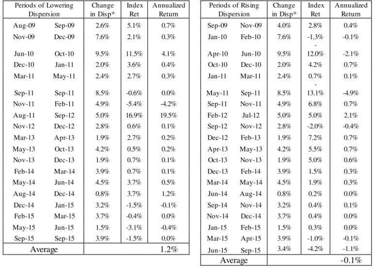
the gauge and comparison of the index total return amid period of rising and lowering dispersion
Reference
1. The Cross-sectional Dispersion of Stocks Returns, Alpha and the Information Ratio. Larry R. Gorman, Steven G. Sapra, Robert A. Weigand. 2010.
2. The role of cross -sectional dispersion in active portfolio management. Larry R. Gorman, Steven G. Sapra, Robert A. Weigand. 2010.
3. Picking stocks in a low return dispersion market.
Kostin, Pahstan, Timcenko, Sneider, Snider, Sanchez, Menon. 2015. 4. Cross-sectional return dispersion and the equity premium.
Paulo Maio. 2015.
5. Generating alpha in a world of high correlation and low dispersion. Kostin, Pahstan, Timcenko, Sneider, Snider, Sanchez, Menon. 2015.
Appendix
0% 20% 40% 60% 80%
0% 20% 40% 60% 80%
100% Ex.1 - Cons. Discretionary - Correlation (LHS) Vs R^2 (RHS)
Average Pairwise Correlation Average R^2
0% 20% 40% 60% 80% 100%
0% 20% 40% 60% 80%
100% Ex.2 - Financials - Correlation (LHS) Vs R^2 (RHS)
Table1
Full Disp
Consumer Discretionary
Consumer
Staples Energy Financials Utilities Healthcare Industrials
Info
Tech Materials Telecom.
Beta -0.1 -1.0 -2.3 0.14 -1.46 -1.3 -2.0 0.3 -0.3 -0.3
T-stat -6.3 -35.4 -87.1 -0.1 -34.5 -57.2 -47.1 11.8 -9.4 -9.9
Table2
Disp Score
Consumer Discretionary
Consumer
Staples Energy Financials Utilities Healthcare Industrials
Info
Tech Materials Telecom.
Beta -0.4 -1.8 -2.5 -0.2 -3.2 -1.3 -1.7 -0.3 -0.2 -1.6
T-stat -19.6 -49.8 -28.2 -0.15 -41.4 -46.1 -43.1 -6.4 -4.5 -24.9
0% 10% 20% 30% 40% 50% 60%
Ex.3 -Cons Disc -Actual Dispersion VS Dispersion Score
Actual Full Dispersion Average Dispersion Score
0% 20% 40% 60% 80% 100%
Ex.4- Financials -Actual Dispersion VS Dispersion Score
0% 20% 40% 60% 80% 100%
0% 20% 40% 60% 80% 100%
Ex.5 - Financials - Corr(LHS) Vs Full Disp (RHS)
Average Pairwise Corr Average Full Disp
0% 20% 40% 60%
0% 50%
100% Ex.6 - Cons Disc - Corr (LHS) Vs Full Disp (RHS)
Average Pairwise Corr Average Full Disp
0% 10% 20% 30%
0% 20% 40% 60% 80% 100%
8/5/2009 8/5/2010 8/5/2011 8/5/2012 8/5/2013 8/5/2014 8/5/2015
Ex.7 - S&P100 - Correlation (LHS) Vs Full Disp (RHS)
Ex.8 – S&P100 – 1month Rolling Dispersion Betas
0% 5% 10% 15% 20% 25% 30%
-20% 0% 20% 40% 60%
8/5/2009 8/5/2010 8/5/2011 8/5/2012 8/5/2013 8/5/2014 8/5/2015
Ex.9 - S&P100 -Full Disp (LHS) Vs Alpha
Average Alpha Full Dispersion - BL
-100% -80% -60% -40% -20% 0% 20% 40% 60% 80%
8/5/2009 8/5/2010 8/5/2011 8/5/2012 8/5/2013 8/5/2014
0% 5% 10% 15% 20% 25% 30%
0.0% 10.0% 20.0% 30.0% 40.0% 50.0% 60.0%
8/5/2009 8/5/2010 8/5/2011 8/5/2012 8/5/2013 8/5/2014 8/5/2015
Ex.11 -S&P100 - VIX Index VS Full Dispersion (RHS)
VIX Average Full Disp
0% 5% 10% 15% 20% 25% 30%
Ex.12 - S&P100 - Dispersion Score Vs Full Dispersion
Average Disp Score Average Full Disp
0% 50% 100%
7/7/2009 7/7/2010 7/7/2011 7/7/2012 7/7/2013 7/7/2014 7/7/2015
Ex.13 - S&P100 - Corr Vs R^2
Table 3 Table4 0% 5% 10% 15% 20% 25% 30%
8/5/2009 8/5/2010 8/5/2011 8/5/2012 8/5/2013 8/5/2014 8/5/2015
Ex.14 -S&P100 - Actual Micro Stdev VS EWMA estimates
Average Actual Micro Stdev Average EWMA Estimate Periods of Lowering
Dispersion Change in Disp* Index Ret Annualized Return
Periods of Rising Dispersion Change in Disp* Index Ret Annualized Return
Aug-09 Sep-09 2.6% 5.1% 0.7% Sep-09 Nov-09 4.0% 2.8% 0.4%
Nov-09 Dec-09 7.6% 2.1% 0.3% Jan-10 Feb-10 7.6% -1.3% -0.1%
Jun-10 Oct-10 9.5% 11.5% 4.1% Apr-10 Jun-10 9.5%
-12.0% -2.1%
Dec-10 Jan-11 2.0% 3.6% 0.4% Oct-10 Dec-10 2.0% 4.2% 0.7%
Mar-11 May-11 2.4% 2.7% 0.3% Jan-11 Mar-11 2.4% 0.7% 0.1%
Sep-11 Sep-11 8.5% -0.6% 0.0% May-11 Sep-11 8.5%
-13.1% -4.9%
Nov-11 Feb-11 4.9% -5.4% -4.2% Sep-11 Nov-11 4.9% 6.8% 0.7%
Aug-11 Sep-12 5.0% 16.9% 19.5% Feb-12 Jul-12 5.0% 5.0% 2.1%
Nov-12 Dec-12 2.8% 0.6% 0.1% Sep-12 Nov-12 2.8% -2.0% -0.4%
Mar-13 Apr-13 1.9% 2.7% 0.2% Dec-12 Feb-13 1.9% 7.2% 0.7%
May-13 Oct-13 4.2% 0.5% 0.2% Apr-13 May-13 4.2% 5.5% 0.7%
Nov-13 Dec-13 1.9% 0.7% 0.1% Oct-13 Nov-13 1.9% 5.0% 0.6%
Feb-14 Mar-14 3.9% 0.7% 0.1% Dec-13 Feb-14 3.9% 1.5% 0.3%
May-14 Jun-14 4.5% 3.7% 0.5% Mar-14 May-14 4.5% 1.9% 0.3%
Aug-14 Dec-14 0.8% 3.7% 1.2% Jun-14 Aug-14 0.8% 0.2% 0.0%
Dec-14 Jan-15 3.2% -1.5% -0.1% Sep-14 Nov-14 3.2% 0.4% 0.1%
Feb-15 Mar-15 3.7% -0.4% 0.0% Nov-14 Dec-14 3.7% 0.4% 0.0%
May-15 Jun-15 1.5% -3.1% -0.4% Jan-15 Feb-15 1.5% 0.3% 0.0%
Sep-15 Sep-15 3.9% -1.5% 0.0% Mar-15 Apr-15 3.9% -1.0% -0.1%
Average 1.2% Jun-15 Sep-15 3.4% -4.2% -1.1%
# firms invested
Total Return Annualized Return Annualized Volatility Ret/Risk Ratio
Long
only Long/Short Index
Long
only Long/Short Index
Long
only Long/Short Index
Long
only Long/Short Index
10 94.2% 67.7% 83.2% 11.0% 8.5% 10.0% 18.2% 15.9% 15.2% 0.60 0.53 0.66
20 95.3% 77.7% 83.2% 11.1% 9.4% 10.0% 16.4% 14.1% 15.2% 0.68 0.67 0.66
30 85.6% 63.0% 83.2% 10.2% 8.0% 10.0% 16.7% 13.9% 15.2% 0.61 0.57 0.66
40 103.7% 82.2% 83.2% 11.8% 9.9% 10.0% 16.4% 13.7% 15.2% 0.72 0.72 0.66
50 107.3% 87.5% 83.2% 12.1% 10.4% 10.0% 16.4% 13.7% 15.2% 0.74 0.76 0.66
60 98.4% 76.9% 83.2% 11.4% 9.4% 10.0% 16.0% 13.4% 15.2% 0.71 0.70 0.66
70 93.2% 71.3% 83.2% 10.9% 8.8% 10.0% 15.8% 13.2% 15.2% 0.69 0.67 0.66
80 92.3% 72.0% 83.2% 10.8% 8.9% 10.0% 15.6% 13.0% 15.2% 0.69 0.68 0.66
90 90.7% 70.4% 83.2% 10.7% 8.7% 10.0% 15.5% 13.0% 15.2% 0.69 0.67 0.66
100 89.5% 70.4% 83.2% 10.6% 8.7% 10.0% 15.5% 13.0% 15.2% 0.68 0.67 0.66
Ex.15 - #50 firms Long only VS S&P100 Index
80 100 120 140 160 180 200 220 240 0 5 -0 8 -2 0 0 9 0 5 -1 1 -2 0 0 9 0 5 -0 2 -2 0 1 0 0 5 -0 5 -2 0 1 0 0 5 -0 8 -2 0 1 0 0 5 -1 1 -2 0 1 0 0 5 -0 2 -2 0 1 1 0 5 -0 5 -2 0 1 1 0 5 -0 8 -2 0 1 1 0 5 -1 1 -2 0 1 1 0 5 -0 2 -2 0 1 2 0 5 -0 5 -2 0 1 2 0 5 -0 8 -2 0 1 2 0 5 -1 1 -2 0 1 2 0 5 -0 2 -2 0 1 3 0 5 -0 5 -2 0 1 3 0 5 -0 8 -2 0 1 3 0 5 -1 1 -2 0 1 3 0 5 -0 2 -2 0 1 4 0 5 -0 5 -2 0 1 4 0 5 -0 8 -2 0 1 4 0 5 -1 1 -2 0 1 4 0 5 -0 2 -2 0 1 5 0 5 -0 5 -2 0 1 5 0 5 -0 8 -2 0 1 5
Ex.16- #50 firms Long/Short VS S&P100 Index