• Nenhum resultado encontrado

Importance of automatic threshold for image segmentation for accurate measurement of fine roots of woody plants

N/A
N/A
Protected

Academic year: 2021

Share "Importance of automatic threshold for image segmentation for accurate measurement of fine roots of woody plants"

Copied!
6
0
0

Texto

(1)

referát – discussion PaPer

http://www.nlcsk.sk/fj/

Importance of automatic threshold for image segmentation

for accurate measurement of fine roots of woody plants

Význam automatického prahovania na obrazovú segmentáciu

pre presné merania jemných koreňov drevín

Peter Surový

1

*, Cati Dinis

2

, Róbert Marušák

1

, Nuno de Almeida Ribeiro

2

1 Czech University of Life Sciences Prague, Faculty of Forestry and Wood Sciences, Kamýcká 129, CZ – 165 21 Praha 6 – Suchdol, Czech Republic

2 Institute of Mediterranean Agricultural and Environmental Sciences (ICAAM), Universidade de Évora - Pólo Da Mitra Apartado 94, 7002-554, Évora, Portugal

Abstract

The fine roots are considered the key organs for plant survival, growth and productivity. Measurement of fine roots variables is easily and conveniently achieved by means of digital image. The descriptive variables like root area, surface, total length and diameter distribution may be obtained from the image. Analysis of digital image consists from several steps, each of them represents potential source of the error. In this article we want to evaluate the automatic thresholding and its impact on principal variables obtainable from digital scans of the fine roots. We compare 16 different thresholding methods and compare them with the human processed binary images of roots of cork oak (Quercus suber L.). We found some of the thresholding methods perform significantly better than others in the estimation of total projected area however the length estimation error points out a little different order of accuracy.

Keywords: fine roots; digital image; automatic thresholding; comparison of methods Abstrakt

Jemné korene sú považované za kľúčové orgány zabezpečujúce prežitie rastliny, jej rast a produkciu. Merania jemných koreňov sú ľahko a pohodlne vykonávateľné pomocou digitálneho obrazu. Popisné veličiny ako plocha koreňov, ich povrch, celková dĺžka či hrúbková štruktúra sa dajú získať z digitálneho obrazu. Analýza digitálneho obrazu pozostáva z niekoľkých krokov, z ktorých každý predstavuje potenciálny zdroj chyby merania. V tomto článku sa zameriavame na automatickú segmentáciu prahovaním a jej vplyv na veličiny zís-kavané z digitálnych skenov jemných koreňov korkového duba (Quercus suber L.). Porovnávame 16 rôznych prahovacích metód a ich správnosť v porovnaní s binárnymi obrazmi vytvorenými ľudským hodnotiteľom. Zistili sme, že niektoré prahovacie metódy dávajú lepšie výsledky ako ostatné v odhade plochy koreňov, ale pred odhad dĺžky koreňov je poradie metód podľa ich správnosti len mierne odlišné. Kľúčové slová: jemné korene; digitálny obraz; automatické prahovanie; porovnanie metód

*Corresponding author. Peter Surový, e-mail: surovy@fld.czu.cz, phone: +420 22438 3871

1. Introduction

The roots are important organ of the tree since they provide the access to the nutrients, water and in elder age they pro-vide stability and resistance against mechanical imbalance (Kozlowski & Pallardy 1997). The fine roots, despite their short longevity are considered the most essential part of the chemical cycles and beside that, also for example, they signi-ficantly contribute to the carbon balance of the tree (Konôpka et al. 2013). In literature huge interest is demonstrated in image analysis techniques for evaluation of fine roots (Kimura et al. 1999; Bouma 2000). There exist a set of com-mercial software (Delta-T-Scan; RooTracker; WinRHIZO) or freeware and open source software (ImageJ; NIHImage;

Object-Image; ObjectJ; EZ-Rhizo; Root Image Analyzer) for analysis of digitized (scanned) samples of fine roots. Also for minirhizotron image analysis (RMS; MR-RIPL 2.0 & 3.0; MSU ROOTs Tracer; Rootfly; RootView; WR-RIPL 2.0; see Le Bot et al. 2010). Despite the existence of this software, it continues to exist the necessity of giving better responses to

new challenges and new imaging techniques for root asses-sment continues to be developed (French et al. 2009) so new software as well as new software for analysis of root images (DART, SIARCS) (Le Bot et al. 2010).

The measurement of root characteristic can be performed manually or semi-manually, but development of automati-zed algorithms is an issue which many root researchers try to evaluate, in order to reduce the time necessary for image processing and also to avoid the subjective human decisions during measurements process (Ewing & Kaspar 1995; Vamerali et al. 2003). From the available software on the market the software WinRHIZO (Regent instruments, Que-bec, Canada) is currently the most used and is considered the most sophisticated root analysis software (Himmelbauer et al. 2004; Zobel 2008). On the other hand the demonstrated set of non commercial software makes it possible to incor-porate most of the algorithms necessary to obtain the root characteristics (Kimura et al. 1999; Kimura & Yamasaki 2001, 2003).

(2)

Importance of thresholding: The digitalization of root

sample is a performed by normal desktop scanner or by scan-ner with additional TPU unit allowing the illumination from above. The sample preparation and scanning protocol has been discussed in Bouma et al. (2000). Afterwards the seg-mentation of root image by thresholding has been indicated as key step in precise root measurements (Himmelbauer et al. 2004). The choice of the proper threshold value is crucial for the image evaluation, since it separates the pixels belonging to roots from background and in such way influences all sub-sequent measurements. In WinRhizo software for instance, it is possible to choose option of automatic thresholding which has been established as an appropriate choice for the root morphological evaluation (Bauhus & Messier 1999; Bouma et al. 2000; Himelbauer et al. 2004).

Bouma et al. (2000) refers that a proper scanning pro-tocol is much more important than the software used, and that the protocol should thus always be listed; however the authors also stress the importance of proper threshold selection, suggesting that higher threshold values can cause more appropriate length estimation though causing incor-rect diameter measurements. Zobel (2008) mentioned that threshold is the key factor when determining the size of an object in grey levelled images, concluding that none of exis-ting software is capable of adequate analysis of different type of digital images representing the fine roots. Smit et al. (1994) developed automated 3d measurement technique of fine roots. He suggested using histogram based segmentation of roots from background. Richner et al. (2000) demonstra-ted for the segmentation of washed root samples, the grey--level thresholding technique is used most frequently. When using thresholding, the most critical step is to define (to set) the level threshold. In a few cases, two threshold grey--levels are used instead of just one (Smit et al. 1994; Kaspar & Ewing 1997). The two threshold levels define the upper and the lower limit of the range of grey-levels belonging to the roots. When decreasing the threshold grey-level to resolve the thinnest roots in a sample, more background pixels along the root boundaries are classified as object pixels and, thus, the contours of thicker roots will blur and expand. In addi-tion, a great deal of noise may occur in the image as a result of a too low grey-level threshold. Staining roots may eliminate some of the problems involved in thresholding, though not completely. In summary, simple grey-level thresholding is appropriate only if there is a good contrast between roots and background and a uniform lighting of the whole scanning area. Because these requirements are most often not met, it is difficult to visually determine the optimal threshold value (Tollner et al. 1994).

Apart from grey-level thresholding, however, only a very limited number of sophisticated segmentation techniques have been applied in the analysis of washed root systems. Smit et al. (1994) first estimated the background, using local maximum and minimum filters. Before the final histogram--based grey-level thresholding, they applied a Laplacian-like sharpening filter. Sumcker et al. (1987) used a combination of edge enhancement and grey-level thresholding. Koller et al. (1995) proposed a new algorithm for the segmentation and local description of elongated, symmetric line-like struc-tures using a non-linear combination of linear filters. They

adapted and implemented this algorithm into a program which provides local shape attributes (position, width and direction of the centre line) that are necessary for the mor-phological description of root segments directly during the detection of curvilinear objects, i.e., roots.

The segmentation of images with low contrast or images that contain very thin roots may result in root objects that are not completely resoled. If these fragmented roots are mea-sured, length and area is underestimated. In addition, some of these root fragments may not satisfy the length-to-width criteria that are used to eliminate extraneous objects from the image. If root fragments are excluded from the measure-ments in this way, measurement errors increase even more. Therefore image-processing algorithms (Russ 1990) can be applied to improve the segmented images prior to morpholo-gical measurements. Kaspar & Ewing (1997) used so called closing to reduce fragmentation of root objects and to smooth object edges without deleting the small objects fragments. Closing involves dilation followed by erosion, which is the reverse of dilation. It can be generally said that no informa-tion can be given on the comparative accuracy of the different systems, because there are no data on comparisons between image analysis systems or programs. In this article we com-pare 15 different thresholding methods available in ImageJ and compare with the manually segmented images. The error of under estimation and overestimation is discussed and we also study its impact on root length measurements.

2. Methods

Root samples: The roots of 7 young cork oak (Quercus suber L.) plants were separated from soil, cut into similar diameter classes and divided into fine and structural roots. The diame-ter division threshold used was 2 mm. The fine roots were washed in water and stored in plastic bottles in low concen-tration of ethanol.

Scanning: EPSON Expression 10000 XL 3.4 scanner was used with the TPU option. This illumination has proven to be better since no shadows are created and also the thresholding is easier due to the clear. The chosen sampling DPI was 400. Images were stored in bitmap format, RGB 24 bits depth.

Fig. 1. Scanner EPSON Expression 1000XL with TPU in the lid

(left), digital image of scanned roots of cork oak.

Image processing: We use ImageJ software to process images stored in common folder. Each image is converted into grey level through Menu: Image-Type-8bit, than one of the 16 thresholding methods is applied. The methods are descri-bed in ImageJ pages (Landini 2011). Following threholding methods are implemented:

(3)

0 – Default method: a method similar to IsoData Method, 1 – Huang method (Huang & Wang 1995). It is based on uniformity shape measure and evaluates the fuzziness of the image to determine value for threshold.

2 – Intermodes method: (Prewitt & Mendelsohn 1966). The threshold is found as minimum (valley) in bimodel or multimodal histogram. It is supposed that each object to be segmented creates a clear peak around the most frequent grey level value.

3 – IsoData method: (Ridler & Calvard 1978 in Landini 2011). The threshold is defined as a value larger than com-posite average of background and object’s averages. 4- IJ_IsoData method: this method is a different implementa-tion of the previous method (Ridler Calvard 1978 in Landini 2011). The method 3 (IsoData) implements the threshold as threshold = (average background + average objects)/2 while this one uses the average of values above and below G (where G is the searched value). The detailed description of the implementation of this method can be found in source code of ImageJ software.

5 – Li method (Li & Tam 1998). It is based on iterative method for minimization of cross-entropy between segmented and original image. Cross-entropy is understood as a measure alternative to alternative squared error.

6 – MaxEntropy (Kapur et al. 1985) the method is based on original method of enthropy consideration proposed by Pun (1980) (in Kapur et al. 1985) while in Kapur et al. 1985 numerical errors in his formulation were rectified and examples presented.

7 – Mean (Glasbey 1993), the threshold is set as a mean of grey values, this method is sometimes used as a starting threshold value in other methods.

8 – MinError (I) based on Kittler & Illingworth (1986). The value of threshold is derived under assumption of normal distribution of grey level values. It is mostly suitable in mul-tithreshold images.

9 – Minimum (Prewitt & Mendelsohn 1966) This method similarly to the internodes method assumes a bimodal his-togram. The histogram is smoothed until only two local maxima remain.

10 – Moments (Tsai 1985). A method which estimates the threshold in a way that the moments of the input image are preserved in an output image.

11 – Otsu (1979) searches for the threshold that minimizes intra-class variance.

12 – Percentile (Doyle 1962), method assumes the fore-ground pixels to be 0.5

13 – RenyiEntropy (Kapur et al. 1985) uses Renyi Entropy, otherwise similar to Max Entropy method.

14 – Shanbhag (Shanbhag 1994) modification of Kapur (1985) method with a more focus on resulting image. 15 – Triangle (Zack 1977) geometric method which assumes one peak of histogram in near one end and search toward the other end.

16 – Yen (Yen et al. 1995) takes to account two factors, the discrepancy between thresholded and original image and the number of bits required to represent thresholded image. More detailed description can be found in http://fiji.sc/wiki/ index.php/Auto_Threshold

Projected area measurement: The root area is measured as amount of pixels belonging to the thresholded region. It is based on formula: area = (1/dpi)^2, where dpi is value of dots per inch used in scanning in mm. The ImageJ software offers direct calculation of area, after the correct scale setting. Length measurements: Several methods for root length esti-mation can be found in literature. For example (Vamerali et al. 2003) used Fibrelength (FbL) algorithm, which proved to be significantly faster than commonly used skeletonization, however it only provided reliable results with small densities of roots with no overlapping. Probably the most common and easiest method is before the skeletonization of binary image decribed for example in (Berntson 1992) the program presented here processes images by first converting digitized root images into a binary tree data structure which can be analyzed in a variety of ways to characterize the branching patterns and the distribution of link size within root systems. This allows quantification total root length and patterns of branching within root systems using analytical techniques from the analysis of stream drainage networks. The simple counting of pixels remaining after skeletonization can only provide reliable results if the roots are horizontally or verti-cally aligned (Vamerali et al. 2003). In case of diagonally or randomly aligned roots the coefficient of certain value may be applied, for example Smit et al. 1994 proposed value of 1.12. Later Kimura & Yamasaki (2001; 2003) introduced the method for estimation of root length together with Here we propose modified algorithm for length estimation which provide similar results and can be easily implemented in ImageJ macro language. The main idea of using skeleton binary image is to count pixels which remain after skeleto-nization (black pixels). However not each pixel can be coun-ted by the same weight as already mentioned by Smit et al. (1994). On the other hand simple correction coefficient may be too simple to describe all possible situations where the correction is necessary. In Figure X are displayed six possible scenarios of central pixel and possible skeleton neighbours. Using Pythagoras theorem we can estimate the length for each situation:

1 2 3 4 5 6

Situation 1, 3 and 4 the length value will be determined as full horizontal (or vertical) size of the pixel. E.g. if scan-ning dpi is 300, the length will be 25.4/300 = 0.0847 mm. In situations 2 and 5 the length value will be calculated as  = 1.118 (* 0.0847 to convert to mm) = 0.0947. For the situation 6 the length will be calculated as


= 1.414 (* 0.0847 to convert to mm) = 0.1197 mm. For the statistical analysis we used software SPSS 20.

3. Results

The absolute values of results are displayed in Figure 1. In the left part are shown mean errors for area estimations and in the right part it is displayed the error for length estimation based on above mentioned algorithm. The “true” length is estimated from binary images created by human operator.

(4)

Fig. 2. Boxplot of mean error for area estimation (left), and

the mean error of length estimation compared to manually seg-mented images (right). The value for method 12 is out of the scale for axis Y.

We use Friedman Test to calculate the ranking for the indi-vidual methods; the resulting order is displayed in Table 1.

Table 1. Friedman ranking of individual thresholding method (the default

ImageJ method marked in bold).

Error by Method type Ranks

AreaErr_2 (Prewitt & Mendelsohn 1966) 3.69

AreaErr_10 (Tsai 1985) 4.45

AreaErr_3 (Ridler & Calvard 1978) 4.47

AreaErr_11 (Otsu 1979) 4.61

AreaErr_9 (Prewitt & Mendelsohn 1966) 4.63

AreaErr_d (default method) 4.73

AreaErr_4 (Ridler & Calvard 1978) 4.73

AreaErr_5 (Li & Tam 1998) 4.97

AreaErr_1 (Huang & Wang 1995) 9.11

AreaErr_13 (Kapur et al. 1985) 10.59

AreaErr_6 (Kapur et al. 1985) 10.67

AreaErr_16 (Yen et al. 1995) 12.19

AreaErr_8 (Kittler & Illingworth 1986) 13.13

AreaErr_7 (Glasbey 1993) 14.50

AreaErr_15 (Zack 1977) 14.69

AreaErr_14 (Shanbhag 1994) 14.84

AreaErr_12 (Doyle 1962) 17.00

We use the K-means cluster technique to divide the data into two groups which may be interpreted as a classification into “good” and “bad” thresholding techniques classes. The “bad” group starts with AreaErr_1 the error in area estima-tion by method 1.

The accuracy of each method is composed of two prin-cipal errors:

1 – over estimation: the pixel is defined as the root pixel in analysed image, but in true image it is background

2 – under estimation: pixel is defined as background image, though in true image it is root.

Both errors may be considered incorrect though in case of equivalent over and under estimation the area may be OK

The best indicator of this error is ratio over/under esti-mation displayed in table 2. The value above 1 indicates that the method produce more overestimation pixels than underestimation pixels. The value close to 1 indicates the equal production of these two errors, while values under one indicate that the underestimation prevails. We calcu-late the ranking based on this index. The interpretation of this value should be in a sense that the highest the position the more the underestimation prevails and the opposite. The methods positioned in the middle of the table are those with

more balanced over and underestimation which is possibly correlating with the precise length estimation (however it does not mean the correct position of the root was found it might have been displaced equally so the over and underesti-mation are similar).

Table 2. Ratio between over- and under-estimation (the default

ImageJ method marked in bold).

Error by Method type Ranks Mean

index15 (Zack 1977) 2.38 0.013

index7 (Glasbey 1993) 2.59 0.014

index12 (Doyle 1962) 3.13 0.034

index16 (Yen et al. 1995) 4.47 0.042

index8 (Kittler & Illingworth 1986) 5.69 8.313

index6 (Kapur et al. 1985) 5.95 0.051

index13 (Kapur et al. 1985) 6.03 0.051

index1 (Huang & Wang 1995) 7.48 0.235

index10 (Tsai 1985) 10.36 1.648

indexD (default method) 10.70 2.038

index4 (Ridler & Calvard 1978) 10.70 2.038

index11 (Otsu 1979) 11.08 2.056

index3 (Ridler & Calvard 1978) 11.22 2.086

index2 (Prewitt & Mendelsohn 1966) 14.16 4.189

index9 (Prewitt & Mendelsohn 1966) 14.97 6.041

index5 (Li & Tam 1998) 15.69 7.867

index14 (Shanbhag 1994) 16.41 —

Length estimation and impact of thresholding on correct length estimation. One of the most important variables for root studies is the total length of the sample. The accuracy of length estimation depends on correct shape extraction by thresholding. While during area estimation (especially when under and over estimation is balanced) the accuracy may be good, compared to human observer, in case of length there is necessity for the shape to be as much similar as possible to the real one.

Table 3 shows the rankings for individual methods cal-culated by Friedman test. It is possible to observe that the method 10 is considered as the best method in error esti-mation.

Table 3. Ordering of methods by ranking estimation for length

measurements (the default ImageJ method marked in bold).

Error by Method type Ranks

Len_err_10 (Tsai 1985) 3.73

len_err_d (default method) 3.92

Len_err_4 (Ridler & Calvard 1978) 3.92

Len_err_11 (Otsu 1979) 4.05

Len_err_3 (Ridler & Calvard 1978) 4.19

Len_err_1 (Huang & Wang 1995) 4.61

Len_err_2 (Prewitt & Mendelsohn 1966) 6.50

Len_err_9 (Prewitt & Mendelsohn 1966) 7.44

Len_err_5 (Li & Tam 1998) 8.03

Len_err_13 (Kapur et al. 1985) 10.16

Len_err_6 (Kapur et al. 1985) 10.17

Len_err_16 (Yen et al. 1995) 12.19

Len_err_8 (Kittler & Illingworth 1986) 13.31

Len_err_14 (Shanbhag 1994) 14.41

Len_err_7 (Glasbey 1993) 14.63

Len_err_15 (Zack 1977) 14.75

(5)

4. Discussion and conclusions

The automatic image analysis methods for root studies are of essential importance due to the large amount of samples usu-ally being evaluated in the studies. The target variables to be measured are the root area, root length, the classification of roots into diameter classes, the amount of root tips, forks and other. The first two mentioned variables (area and length) are the main aim of this study and especially the automatic estimation of them.

In order to automatically estimate the values the fol-lowing steps need to be executed: digitization of roots into raster image, segmentation by threshold, counting the pixels belonging to roots, skeletonization and estimation of length. The digitization is done by a scanner in which the sample is spread on the plate, if necessary in the water. The illumi-nation of the roots may be from the bottom (the position of sensor), but it has been demonstrated that more reliable results are obtained if the light source is above the sample, e.g. in the upper lid of scanner. Such scanners are commer-cially available, and usually they are used for scanning of negative film material. The main advantage of illumination from above is that the root colour is not taken to account for the automatic image analysis, and the only values coming from scan are the levels of grey and that the shadow is not present. The advantage of colours is that they can be used when working with small plants whose roots are white or transparent and they are difficult to distinguish if they are illuminated from above. The roots of woody plants are usually dark and the root skin (especially when wet) may reflect the light (causing white shiny artefacts) confusing the automatic detection. Therefore for the acquisition of digital images of woody roots the above light is more suitable.

The next step for automatic analysis of roots is the auto-matic segmentation of the images into roots and background. This problematic (the problematic of automatic threshol-ding) is the main purpose of this study. The following pro-cedures, after segmentation, are area assessment which is the sum of pixels defined as roots, then morphological analysis: length estimation and others. We compare the automatically calculated threshold levels to human processed binary ima-ges e.g. imaima-ges which were manually segmented into roots and background, not using threshold but manual pixel iden-tification. The operators were asked to paint the roots on the image by black colour and the rest (background) was filled by white colour. The main reason for this kind of process was to avoid possible errors caused by the thresholding method itself.

As it can be seen from tables 1–3 the two best methods considered for area estimation are methods 2 (Prewitt & Mendelsohn 1966) and 10 (Tsai 1985). The K–means cluste-ring into two groups (better and worse) indicates that several methods are suitable for area estimation including 2 (Prewitt & Mendelsohn 1966), 10 (Tsai 1985), 3 (Ridler & Calvard 1978), 11 (Otsu 1979), 9 (Prewitt & Mendelsohn 1966), default, 4 (Ridler & Calvard 1978) and 5 (Li & Tam 1998). All these methods provide reliable estimates of projected area of roots compared with the human observer. The principal danger, especially when using the global threshold values, which is kind of context unaware, is that the area may be

dis-placed to the shadow or blurry parts and in such way the total area value may be correct, however its incorrect positioning may cause errors in subsequent processing.

Therefore the error of over and underestimation was evaluated pixel by pixel in table 2. The error is displayed in column Mean. Closer the value is to number 1, the better is the fit of the pixels estimated by automatic procedure and those marked by the human observer. The values below 1 indicates that there is the underestimation e.g. the values are marked as the background however they should be marked as the roots. The values over 1 indicates opposite of this situ-ation, e.g. the pixels are marked as the roots however they should be marked as the background. It can be observed that the method 10 (Tsai 1985) is the one closest to the value of 1 so its accuracy in terms of over and under estimation is most likely the best.

The mentioned result is also reflected in the table 3 where the length error estimation is displayed. The method number 10 (Tsai 1985) is the best method for assessment of length from binary images and other methods from the upper half of the table (methods default, 4 (Ridler & Calvard 1978), 11 (Otsu 1979), 3 (Ridler & Calvard 1978), 1 (Huang & Wang 1995), 2 (Prewitt & Mendelsohn 1966), 9 (Prewitt & Men-delsohn 1966) and 5 (Li & Tam 1998)) are considered better (more recommended) as the other half. We used approxi-mate estimation of the length from skeletonized images. We found out that some method perform better than others and clustered them into two groups which may be interpreted as good and bad methods for root image thresholding. The one method which appears to be the most accurate (however not significantly more than the other methods in the “good” group) is the method of moments described in Tsai (1985). As already mentioned by Bouma et al. (2000) the scan-ning protocol is very important to avoid subjective decisions during the root measurement process. The root staining, following (Tollner et al. 1994) may enhance the visibility of roots, though nowadays the most common technique to improve the contrast between roots and background is the use of above light, so called TPU (transparency unit). This kind of scanner is common on the market. We showed that even when using TPU however, the values of automatic threshold will vary based on the method used to calculate it and so it is important to choose the most suitable one. The evolution of devices for image acquisition nowadays, and the simultaneous advances in computer vision (with other algorithms for automatic image analysis) suggest that the use of digital images for measurements is promising and its potential will increase very probably in the near future.

References

Ansari, S., A., Kumar., P., Gupta., B. N., 1995: Root surface area measurements based on adsorption and desorption of nitrite. Plant and Soil, 175:133–137.

Bauhus, J., Messier, C., 1995: Evaluation of Fine Root Length and Diameter Measurements Obtained Using RHIZO Image Analy-sis. Agronomy Journal, 28:142–147.

Berntson, G. M., 1992: A computer program for characterizing root system branching patterns. Plant and Soil, 140:145–149.

(6)

Bouma, T. J., Nielsen, K. L., Koutstaal, B., 2000: Sample prepara-tion and scanning protocol for computerised analysis of root length and diameter. Plant and Soil, 218:185–196.

Costa, C., Dwyer, L., M., Hamilton, R. I., Hamel, C., Nantais, L., Smith, D. L., 2000: A Sampling Method for Measurement of Large Root Systems with Scanner-Based Image Analysis. Agronomy Journal, 4:621–627.

Doyle, W., 1962: Operation useful for similarity-invariant pattern recognition. Journal of the Association for Computing Machin-ery, 9:259–267.

Ewing, R. P., Kaspar, T. C., 1995: Accurate perimeter and length measurement using an edge chord algorithm. Journal of Com-puter-Assisted Microscopy, 7:91–100.

French, A., Úbeda-Tomás, S., Holman, T. J., Bennett, M. J., Prid-more, T. P., 2009: High throughput quantification of root growth using a novel image analysis tool. Plant Physiology, 150:1784–1795.

Glasbey, C. A., 1993: An analysis of histogram-based thresholding algorithms, CVGIP: Graphical Models and Image Processing, 55:532–537.

He, W., Nakayama, K., Yu, G., 1998: The effect of root surface area on the water uptake and transpiration rate of maize plants. Technical bulletin- faculty of horticulture Chiba University, 52:157–164.

Himmelbauer, M. L., Loiskandl, W., Kastanek, F., 2004: Estimat-ing length, average diameter and surface area of roots usEstimat-ing two different Image analyses systems. Plant and Soil, 260:111–120. Huang, L. K., Wang, M. J. J., 1995: Image thresholding by minimi-zing the measures of fuzziness. Pattern recognition, 28:41–51. Jackson, R. B., Mooney, H. A., Schulze, E. D., 1997: A global bud-get for fine root biomass, surface area, and nutrient contents. Proceedings of the National Academy of Sciences of the United States of America, 94:7362–7366.

Kapur, J.N., Sahoo, P. K., Wong, A. C. K., 1985: A New Method for Gray-Level Picture Thresholding Using the Entropy of the His-togram. Graphical Models and Image Processing, 29:273–285. Kaspar, T. C., Ewing, R. P., 1997: ROOTEDGE: software for mea-suring root length from desktop scanner images, Agronomy Journal, 89:932–940.

Kimura, K., Kikuchi, S., Yamasaki, S., 1999: Accurate root length measurement by image analysis. Plant and Soil, 216:117–127. Kimura, K., Yamasaki, S., 2001: Root length and diameter mea-surement using NIH Image: application of the line-intercept principle for diameter estimation Plant and Soil, 234:37–46. Kimura, K., Yamasaki, S., 2003: Accurate root length and diameter

measurement using NIH Image: use of Pythagorean distance for diameter estimation Plant and Soil, 254:305–315. Kittler, J., Illingworth, J., 1986: Minimum error thresholding,

Pat-tern Recognition. 19:41–47.

Konôpka, B., Pajtík, J., Maľová, M., 2013: Fine root standing stock and production in young beech and spruce stands. Lesnícky časopis - Forestry Journal, 59:163–171.

Kozlowski, T. T., Pallardy, S. G., 1997: Physiology of Woody Plants. San Diego, Academic Press, 411 p.

Landini, G., 2011: AutoThreshold pluging for ImageJ. Availabe at: http://fiji.sc/wiki/index.php/Auto_Threshold (accessed online 7.11.2014)

Li, C. H., Tam, P. K. S., 1998: An iterative algorithm for minimum cross entropy thresholding. Pattern Recognition Letters. 19:771–776.

Le Bot, J., Serra, V., Fabre, J., Draye, X., Adamowicz, S., Pagès, L., 2010: DART: a software to analyse root system architec-ture and development from caparchitec-tured images Plant and Soil, 326:261–273.

Otsu, N., 1979: A threshold selection method from gray-level histo-grams, IEEE Transactions on Systems, Man, and Cybernetics, 9:62-66.

Pregitzer, K. S., Deforest, J. L., Burton, A., J., Allen, M. F., Ruess, R. W., 2002: Fine Root Architecture of Nine North American trees Ecological Monographs, 2:293–309.

Prewitt, J. M. S., Mendelsohn, M. L., 1966: The analysis of cell ima-ges. Annals of the New York Academy of Sciences, 128:1035– 1053.

Regent Instuments, 1996: WinRHIZO V3.9 Reference. Regent Instruments Inc., Quebec, Canada.

Richner et al., 2000: Root image analysis and interpretation In: Smit et al (ed.): Root methods a Handbook, p. 305–341.

Shanbhag, Abhijit, G., 1994: Utilization of information measure as a means of image thresholding, CVGIP: Graphical Models and Image Processing, 56: 414–419.

Simojoki, A., 2000: Calibration of a desktop scanner and digital image analysis procedure for quantification of root morphology Agricultural and Food Science, 9:223–230.

Smit, A. L., Sprangers, J. F. C. M., Sablik, P. W., Groenwold, J., 1994: Automated measurement of root length with a three--dimensional high-resolution scanner and image analysis Plant and Soil, 158:145–149.

Tanaka, S., Yamauchi, A., Kono, Y., 1995: Easily accessible method for root length measurement using an image analysis system, Japanese Journal of Crop Science, 1:144–147.

Tsai, W., 1985: Moment-preserving thresholding: a new approach, Computer Vision, Graphics, and Image Processing, 29:377– 393.

Vamerali, T., Guarise, M., Ganis, A., Bona, S., Mosca, G., 2003: Analysis of root images from auger sampling with a fast pro-cedure: a case of application to sugar beet. Plant and Soil, 255: 387–397.

Yen, J. C., Chang, F. J., Chang, S., 1995: A New Criterion for Auto-matic Multilevel Thresholding, IEEE Transactions on Image Processing, 4:370–378.

Zack, G. W., Rogers, W. E., Latt, S. A., 1977: Automatic measure-ment of sister chromatid exchange frequency, Journal of His-tochemistry & CyHis-tochemistry, 25:741–53.

Zobel, R. W., 2008: Hardware and software efficacy in assessment of fine root diameter distributions Computers and Electronics in Agriculture, 60:178–189.

Imagem

Fig. 1. Scanner EPSON Expression 1000XL with TPU in the lid  (left), digital image of scanned roots of cork oak.
Table 3 shows the rankings for individual methods cal- cal-culated by Friedman test. It is possible to observe that the  method 10 is considered as the best method in error  esti-mation

Referências

Documentos relacionados

2 Para Vico a corrupta natureza do homem ocorre em razão do pecado original, e com essa corrupta natureza: “percebemos com toda claridade que esta, não só nos

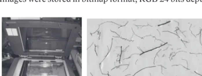
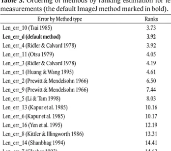
improving the texture segmentation. The effect of image segmentation depends on the color values to a certain extent. Given the complicated light conditions and background of

We also determined the critical strain rate (CSR), understood as the tangent of the inclination angle between the tangent to the crack development curve and the crack development

It engages in advance thinking and early politi- cal-strategic planning of possible CSDP responses to crises, incorporating both the civilian and the military

Essas declarações prospectivas podem «acreditar», «planejar» ou «estimar», bem como por outros documento foram obtidas de fontes públicas por nós consideradas é assegurada de

60 Cfr. Escobar Fomos, Iván, Manual de Derecho Constitucional, 2a. Abad Yupanqui, Samuel, “El Ombudsman o Defensor del Pueblo en la Constitución peruana de 1993; retos y

Resumo Com início em 2011 a União Europeia atravessou uma crise migratória sem precedentes, desde a II Guerra Mundial, que traz consigo uma série de consequências para a

Nesse contexto, o psicólogo é identificado como profissional que deve estar capacitado em sua formação, conhecer o fenômeno com o qual está lidando, proporcionar