PREDICTING SOCCER OUTCOME WITH
MACHINE LEARNING BASED ON WEATHER
CONDITION
PREDICTING SOCCER OUTCOME WITH MACHINE
LEARNING BASED ON WEATHER CONDITION
Dissertation supervised by: Francisco Ramos , PhD
Universitat Jaume I, Castellon de la Plana, Spain
Co-supervised by: Roberto Henriques, PhD Universidade Nova de Lisboa,
Lisbon, Portugal
Co-supervised by: Prof. Jorge Mateu Universitat Jaume I, Castellon de la Plana, Spain
ACKNOWLEDGMENTS
The idea about this research start from a small conversation between me and Francisco Ramos on February 2018. He told about his idea of making a system to predict the outcome of soccer matches using weather data with the machine learning algorithm, this topic is very interesting for me since I like to watch soccer matches and at the same time I also curious to learn about machine learning. At first, I am not confident to take this topic since I consider myself not have enough mathematics background, but he convincing me that I have the capability to do this topic. So I would like to thank Francisco Ramos for belief in me and all the help that you provide during the process of this research.
I also would like to thank Joaquin Torres for all of the tutorships that you provide me about machine learning. He spends so much time to teach me even though he is not one of my supervisors and for that I am really grateful.
I also want to thank my classmates and flatmate. Thank you for all of your support in every aspect to keep me moving forward.
Finally, I would like to thank my family and friends in Indonesia. Thanks for keeping in contact with me regularly even though we are all living in different time zone and separate for thousands of miles. My study finally comes to an end and I can’t wait to meet all of you when I return to Indonesia.
PREDICTING SOCCER OUTCOME WITH MACHINE
LEARNING BASED ON WEATHER CONDITION
ABSTRACT
Massive amounts of research have been doing on predicting soccer matches using machine learning algorithms. Unfortunately, there are no prior researches used weather condition as features. In this thesis, three different classification algorithms were investigated for predicting the outcomes of soccer matches by using temperature difference, rain precipitation, and several other historical match statistics as features. The dataset consists of statistic information of soccer matches in La Liga and Segunda division from season 2013-2014 to 2016-2017 and weather information in every host cities. The results show that the SVM model has better accuracy score for predicting the full-time result compare to KNN and RF with 45.32% for temperature difference below 5° and 49.51% for temperature difference above 5°. For over/under 2.5 goals, SVM also has better accuracy with 53.07% for rain precipitation below 5 mm and 56% for rain precipitation above 5 mm.
KEYWORDS
Weather Soccer Football Machine Learning K-nearest neighborsSupport vector machine
ACRONYMS
ML Machine learning
KNN K-nearest neighbors
SVM Support vector machine
RF Random forest
INDEX OF THE TEXT
ACKNOWLEDGEMENT... iii
ABSTRACT ... iv
KEYWORDS ... v
ACRONYMS ... vi
INDEX OF THE TEXT ... vii
INDEX OF TABLES ... ix INDEX OF FIGURES ... x 1. INTRODUCTION ... 1 1.1. Background ... 1 1.2. Research Objectives ... 2 1.3. Assumptions ... 2
2. BACKGROUND AND RELATED WORKS ... 3
2.1. Soccer ... 3
2.2. Weather ... 3
2.3. Machine Learning ... 3
2.3.1. Supervised Classification Algorithms ... 4
2.4. Measuring Performance ... 8
2.4.1. Confusion Matrix ... 8
2.4.2. Classification Ratio ... 9
2.5. Betting Odds ... 9
2.6. Predicting Soccer Matches Outcome ... 10
2.6.1. Challenges of Predicting Soccer Matches ... 10
2.6.2. Related Works ... 10
3. METHODOLOGY ... 15
3.1. Hardware and Software ... 15
3.2. Data Sources ... 16
3.3. Features and Labels ... 19
3.4. Data Preprocessing ... 21
3.5. Data Splitting and K-Fold Cross-Validation ... 21
3.6. Hyperparameter Optimization ... 22
4.1. Dataset and Features ... 25
4.2. Best Hyperparameters ... 27
4.3. Confusion Matrix ... 31
4.4. Model Accuracy ... 35
4.5. Misclassification Rate ... 38
4.6. Comparison with betting odds ... 40
5. CONCLUSION ... 41
REFERENCES ... 42
INDEX OF THE TABLES
Table 2.1: Example of confusion matrix binary classification ... 8
Table 2.2: List of previous works ... 12
Table 3.1: All software used during the thesis project ... 16
Table 3.2: The computer specifications used for training the model ... 16
Table 3.3: List of historic features with description ... 20
Table 3.4: List of WEATHER features with description... 20
Table 3.5: Overview of how the data is partitioned ... 21
Table 3.6: The list of parameters and their values for KNN, SVM, and RF algorithms. ... 23
Table 4.1: Number of matches for dataset with rain precipitation below and above 5° …… ... 25
Table 4.2: Number of matches for dataset with rain precipitation below and above 5 mm. ... 26
Table 4.3: List of features for case study 1 and 2 ... 26
Table 4.4: Result of hyperparameter optimization of KNN model for matches above and below 5° temperature difference ... 27
Table 4.5: Result of hyperparameter optimization of SVM model for matches above and below 5° temperature difference ... 27
Table 4.6: Result of hyperparameter optimization of RF model for matches above and below 5° temperature difference ... 27
Table 4.7: Result of hyperparameter optimization of KNN model for matches above and below 5 mm rain precipitation ... 29
Table 4.8: Result of hyperparameter optimization of SVM model for matches above and below 5 mm rain precipitation ... 30
Table 4.9: Result of hyperparameter optimization of RF model for matches above and below 5 mm rain precipitation ... 31
Table 4.10: Proportion of FTR correctly predicted for each model ... 35
Table 4.11: Proportion of over/under 2.5 goals correctly predicted for each model . 37 Table 4.12: Misclassification rate of FTR prediction for each models ... 38
Table 4.13: Misclassification rate of over/under 2.5 for prediction for each models 39 Table 4.14: Prediction accuracy of bookmakers ... 40
INDEX OF FIGURES
Figures 2.1: RF architecture [Verikas et al. (2011)] ... 5
Figures 2.2: The 1-, 2- and 3- nearest neighbors [Mulak & Talhar (2015)] ... 5
Figures 2.3: Example of SVM classification [Karthikeyan et al. (2016)]. ... 7
Figures 3.1: Flowchart to visualize the methodology of the thesis ... 15
Figure 3.2: Pie chart to visualize the distribution of FTR of the dataset ... 17
Figure 3.3: Pie chart to visualize the distribution of over/under 2.5 goals of the dataset ... 17
Figure 3.4: The screenshot of AEMT csv file. ... 18
Figure 3.5: The process from raw data into classification result. ... 19
Figure 3.6: K-fold cross-validation visualization with k=10. ... 22
Figure 4.1: Confusion Matrices of FTR prediction using KNN, SVM, and RF models. ... 32
Figure 4.2: Confusion Matrices of over/under 2.5 goals prediction using KNN, SVM, and RF models. ... 33
Figure 4.3: Bar chart to visualize accuracy of each model for FTR prediction. ... 35
Figure 4.4: Bar chart to visualize accuracy of each model for over/under 2.5 goals prediction.. ... 37
1.
INTRODUCTION
1.1.
Background
Soccer is currently the most popular team sport [Total Sportek (2016)]. The 2018 edition of FIFA World Cup was broadcast live to every territory around the world with an estimated 3.572 billion viewers watch the event [FIFA (2018)]. With such a large amount of attention, the soccer forecast has a huge potential to become a profitable business. Sportradar director Darren Small states that the industry of match-betting of sports have estimated value of $700 billion to $1 trillion annually a year which 70% of that trade has been estimated to come from soccer betting [Keogh & Rose (2013)]. The easy access to the Internet can be considered as the main reason for the growing revenue of the betting industry since people can just use electronic devices that connected to the internet to bet online. Due to the increase amount of financial involved in the sport-betting industry, predicting the final outcome of the match become more important than ever; thus bookmakers, fans, and gamblers are all interested to make prediction of a match in before the match started [Bunker & Thabtah (2017)]. Concurrent with the enthusiastic increase of the soccer-betting industry, more people become enthusiasm to do research on soccer forecast.
Soccer gambler usually prefer betting on predicting the full-time result (FTR) even though there are also other kinds of outcome that users can bet such as total goals, goalscorer, halftime result and so on. There are three possible outcome of FTR which are home team win, draw, and away team win, because of the nature of the outcome, predicting FTR can be categorized as a multiclass classification problem. Another outcome that gamblers like to predict is the number of goals, most of gambler avoid to predict the exact number of goals since it is very hard so as alternative bookmarkers give them an option to predict whether the number of goal will be below or above certain numbers (0.5, 1.5, 2.5, etc), this problem is categorized as binary classification problem. One of the intelligent approaches that have been proven in terms of predicting classification problem is Machine learning (ML) [Bunker & Thabtah (2017)]. In the past, there are many studies were done using various ML method to forecast the result of soccer matches. However, as an outdoor sport soccer players performance can be really affected by the weather and these previous research usually
forget to incorporate weather condition as one of the variables to determine the final result, this is the main motivation of using weather as main parameters for this thesis.
1.2.
Research Objectives
This thesis aims to predict the outcome of soccer matches using ML techniques using weather information as features. The focus will be on determining the FTR and over/under 2.5 goals. Soccer is very unpredictable since there are a lot of factors need to consider such as players quality, location(home or away match), recent form, injuries, and so on.
To fulfill the goal, the specific objectives are:
● To review and evaluate various ML classification algorithms that have the potential to predict the outcome of soccer matches using available dataset. ● To design and implement various ML classification algorithms and optimize
the hyperparameters to improve the accuracy of each algorithm.
● To compare the performance of the various ML classification algorithms in order to find the best model and also compare the accuracy of the models with bookmarkers to find out whether the models have better accuracy than bookmakers or not.
● To conclude how much the effect of temperature difference and rain precipitation can really influence the outcome of soccer matches.
1.3.
Assumptions
The main assumption is the more temperature gap between the match location compare to the away team home base, the more likely home team to win the match. Another assumption is the increase of rain precipitation on the matchday will decrease the number of goals since rain makes the grass wet therefore the ball is harder to control [Byrne (2016)].
2.
BACKGROUND AND RELATED WORKS
In this chapter, the basic rules of soccer will be explained including the potential of weather on affecting the outcome of the soccer matches. Several classification algorithms will also be explained and the past related works within the topic of soccer prediction machine learning modeling.
2.1.
Soccer
Soccer (or most of the people known as football) is a sport game which involves two teams, where each team consists of ten field players and one goalkeeper. Matches can be held on natural or artificial surfaces. Match is controlled by a referee who has full authority to enforce the laws of the game accompany by two assistant referees [FIFA (2018)]. The match lasts totally 90 minutes which separated into two equal periods of 45 minutes and between those two periods there are 15 minutes half-time interval.
2.2.
Weather
Weather is the condition of the atmosphere, describing for example the degree to which it is hot or cold, wet or dry, calm or stormy, clear or cloudy [Merriam-Webster (n.d.)]. Weather usually consist of temperature, rain precipitation, humidity and wind speed. For this thesis, temperature and rain precipitation are used as features. Both temperature and rain can influence an outdoor sport event. For example, One of the research on National Football League (NFL) which is the highest competition on American Football suggesting teams are better at rushing and worse at passing in low temperatures [Zipperman (2014)]. Too much rain can influence on the game especially if the match held in the stadium without drainage system since it may result in standing water which can cause the ball to stick and not move around as easily [Byrne (2016)].
2.3.
Machine Learning
The term machine learning refers to the automatic process to find significant data patterns. In the last decades, ML algorithms become very popular choice to solve any task that requires information extraction from a big data set. Same like human being, the learning process on ML is a process of gaining experience and convert it into
knowledge. In the case of ML, before able to generate knowledge or expertise first it needs to receive experience in the form of training dataset [Shalev-Shwartz & Ben-David (2014)]. There are various kind of ML algorithms, usually these algorithms are grouped into two category; unsupervised and supervised learning. Unsupervised learning is a method to find the pattern of unlabelled dataset which means the dataset have no corresponding output value. In supervised learning, on the other hand, make prediction based on some already known examples or fact(labelled dataset) [Kurama, V. (2018)].
Since this research use labeled dataset, only supervised learning will be evaluated further. Supervised learning problems also divided into "regression" and "classification" problems. The main difference between regression and classification the data type of the label/output. If the label/output value is continuous e.g. home prices then it belong to regression problem while if the label/output value is discrete e.g. gender then it belong to classification. For this thesis, only classification algorithms will be explained further since the output of this research is to predict FTR outcome (home team win, draw, away team win) and over/under 2.5 goals which are discrete value.
2.3.1.
Supervised Classification Algorithms
2.3.1.1.
Random Forest
Random Forest (RF) algorithm is a development of the Classification and Regression Tree (CART) method by applying bootstrap aggregating (bagging) and random feature selection methods. Even though the decision tree algorithm is easy to interpret and not having many parameters to optimize but it is easy to be overfitting. RF algorithm reduces the danger of overfitting is by constructing an ensemble of trees [Shalev-Shwartz & Ben-David (2014)].
Unlike Decision Tree, the RF method combines many trees to make classifications and prediction classes. In RF tree formation is done by doing training sample data. The selection of variables used for split is taken randomly. The classification is executed after all the trees are formed. This classification of RF is taken based on votes from each tree and the most votes are the winners. General architecture of RF can be seen on Figure 2.1.
Figure 2.1: RF architecture [Verikas et al. (2011)]
There are many ways in order to to tune the performance of random forest. The most common way is to increase the number of decision trees that the algorithm creates so the result can be more reliable, the side effect of increasing the number of decision tree is it will slow down the computation process.
2.3.1.2.
K-Nearest Neighbour
K-nearest neighbor is a supervised algorithm learning where results from new instances classified according to the majority of the closest K-neighbor category. For instance, we want to predict whether “a” is “cat” or “dog”, if K=4 and 3 of the closest is “cat” while only one is “dog”. From this result, the conclusion is “a”=”cat” because the majority of 4 closest neighbours of “a” is “cat”. Figure 2.2 show the KNN visualization with 1-, 2- and 3- nearest neighbors.
There are many ways to calculate the distance, for this research we choose three most famous distance formula which are: Euclidian, Minkowski, and Manhattan. Formula for all type of distances are given below.
I. Euclidian ( , ) = 1 ( − )2 II. Minkowski ( , ) = ( 1 | − | )1 III. Manhattan ( , ) = 1 | − |
The advantages of using KNN are it is an simple algorithm to explain and understand. The main disadvantage of the KNN algorithm is that it is a lazy learn which mean the way the algorithm perform classification is by use the training data itself rather than learn from it [Karthikeyan et al. (2016)].
2.3.1.3.
Support Vector Machine
The current standard of Support vector machines (SVM) were implemented by Cortes and Vapnik back in 1995. Bassically, SVM is an algorithm to separate data by using a hyperplane into different groups with same classifier[Petterson & Nyquist (2017)]. For instances, in two dimensions, a hyperplane is a flat one-dimensional subspace(line). In three dimensions, a hyperplane is a flat two-dimensional subspace(plane). In > 3 dimensions, it can be hard to visualize a hyperplane, but the notion of a − 1 dimensional flat subspace still applies [James et al. (2013)]. Figure 2.3 show the example of SVM classification.
Figure 2.3: Example of SVM classification [Karthikeyan et al. (2016)].
Since there are many ways to make hyperplane, The best possible hyperplane can be determine by measure the distance between the support vectors and the hyperplane. The best hyperplane is the one with the largest distance between the hyperplane and the support vectors which can be called maximum margin hyperplane (MMH). The support vectors are the points in the dataset from both classes that are closest to the MMH. The
support vectors allow the algorithm to be memory efficient even with large amounts of
data, as only the vectors need to be saved for future reference [Petterson & Nyquist (2017)].
Beside able to performing linear classification, SVMs can also perform a non-linear classification where it will mapping the input data into high-dimensional feature spaces, this method is known as the kernel function. By using kernel, The best hyperplane between classes can be found by measuring the maximum hyperplane margin between non-linear input spaces and characteristic spaces [Cortes & Vapnik (1995)]. The commonly used kernel functions are:
● Linear kernel
( , ) = ● Polynomial kernel
● Radial Basis Function (RBF) kernel
( , ) = (− || − ||2), ℎ =1
2 2
2.4.
Measuring Performance
After successfully training the models, the next step is to use test data to evaluate the classification performance of the models. Below are several methods that able to evaluate the performance of machine learning classification algorithm [Vuk & Curk (2006)]:
● Receiver Operating Characteristic (ROC) Curves ● Lift Charts
● Calibration Plots ● Confusion Matrix ● Classification Ratios ● Kappa Coefficient
Classification ratios and confusion matrices will be used to evaluate the performance of each model in this thesis.
2.4.1.
Confusion Matrix
Confusion Matrix or sometimes referred as Error matrix is a N x N matrix to portray the performance of the model when predicting a set of test data for which the true values are known [Data School (2014)], N here represent the number of classes of dependent variables. By using Confusion Matrix, it will show the number of misclassification such as the number of predicted data points which ended up in wrong classification. Below is the table 2.1 to show how the confusion matrix looks like
Actual NO TN FP
Actual YES FN TP
Table 2.1: Example of confusion matrix binary classification
● True Positives (TP): These are the case when the model predicted yes (ex: the number of goals is more than 2.5) and the match actually have more than 2.5 goals.
● True Negatives (TN): the model predicted no, and the match actually have less than 2.5 goals.
● False Positives (FP): the model predicted yes, but the match actually have less than 2.5 goals. (Also known as a "Type I error.")
● False Negatives (FN): the model predicted no, but the match actually have more than 2.5 goals. (Also known as a "Type II error.")
The example on table is specific for binary classification problem (ex: 0 or 1, true or false, etc), since FTR is a multiclass classification problem it will show 3x3 matrix instead.
2.4.2.
Classification Ratio
The Accuracy is the proportion of the total number of predictions that were correct !" (%) =#$. $& '"( ) ' )"'' & $!! )*$ ") #$. $& '"( ) ' + ℎ " "' 100
After find the accuracy, then next logical step to do is to calculate the misclassification rate. It is important because sometimes by calculate only accuracy, it can give you false judgement of the model performance especially if the class distribution on the dataset is uneven.
, ' )"'' & " $+ !" (%) =#$. $& ( ' )"'' & " $+ + )"'' #*$ ") #$. $& '"( ) ' + )"'' # 100
2.5.
Betting Odds
Betting odds can be written in many formats. Currently, the most common types of odds are fractional, decimal and American. The names explain how the odds are
written. As for today, Decimal odds are the most popular odds since it offered by almost all bookmakers around the world. This thesis use the historical betting odds of from Bet365 for FTR and Betbrain for over/under 2.5 goals and the format is in decimal, so only decimal odds is explained in this thesis [Online-Betting.me.uk (n.d.)].
Understanding betting odds with a decimal odds system actually quite simple. The system express the amount of money which will be returned to the gambler on a 1 unit stake. 1 unit can refer to 1 pound, 10 pounds or 100 pounds. For example, if Inter Milan is favoured to win at 1.30 and someone bet £200 for Inter Milan to win the match, then if the prediction is correct then he/she will receive back £260 in total (+£60 in profit) [Online-Betting.me.uk (n.d.)].
2.6.
Predicting Soccer Matches Outcome
This part discusses some challenges in predicting the soccer outcome and some previous works of predicting soccer matches using machine learning.
2.6.1.
Challenges of Predicting Soccer Matches
Even though in recent years many classification problems can be solved with machine learning algorithm, It is still very problematic to predict soccer outcome accurately. There are many cases when the underperform team win the match against better team. It is because many unexpected things can happen during the match such as red card, injury, and sometimes it just pure luck especially when better team can’t convert multiple chance into a goal while underperform team score a goal with less chance.
2.6.2.
Related Works
A decent amount of research has been done on soccer prediction using machine learning method. Most of the previous works were also focus on predicting the FTR.
In 2006, Joseph et al were predicting FTR of Tottenham Hotspurs football team for the period 1995-1997 using expert BN model compared with four different ML algorithms. They used features such as the presence of key players in the field, the attacking power of the team, average quality of the team, and the position of key players in the formation. The average classification accuracy of the models was 59.21% [Joseph et al. (2006)].
Engin Esme and Mustafa Kiran in 2018 used football data of super league of Turkey from season 2010/11 to 2015/16. Features such as the market value of the team, standard deviation and probability based on fixed odds (Bet) are used for this research. The best accuracy prediction of the FTR was 57.52% with k-value = 18 [Esme & Kiran (2018)].
Constantinou et al. created the Bayesian network model using the fatigue, team form, strength, and psychological impact as features. The dataset of English Premier League (EPL) for season 1993/94 to 2009/10 used as training dataset and season 2010/11 as testing dataset [Constantinou et al. (2012)].
Albina categorized all features of his models into static and dynamic group. static features are features that not depend on both teams and dynamic features are the other way around. His Random Forest model able to predict with the precision more than 60% [Yezus (2014)].
Researchers from Educational and Research Institute University in Chennai used Artificial Neural Networks model to predict matches between FC Bayern Munich and FC Borussia Dortmund, as the training dataset they used matches between both team during the period 2005 to 2011 and 2011 to 2012 as testing dataset. The accuracy result when predicting goals is better compared to Football Result Expert System(FRES) but when it comes to predicting the winner, the model have more error value compare to FRES [Sujatha et al. (2018)].
Researchers from the University of Chalmers proposed LSTM neural network as solution to predict soccer outcome. They predict not only using data before the match started, but also during the match for every 15 minutes. The accuracy is between 33-45% (depends on architecture) when the match at 0th minute and between 73-86% when the match already pass 90th minute. [Petterson & Nyquist (2017)].
Researchers from Slovak University of Technology using players attribute from the soccer simulation video game combined with other data from actual matches as parameters, they tried LSTM classification and regression models with the most accurate prediction coming from LSTM regression model with 52.479% [Danisik et al. (2018)].
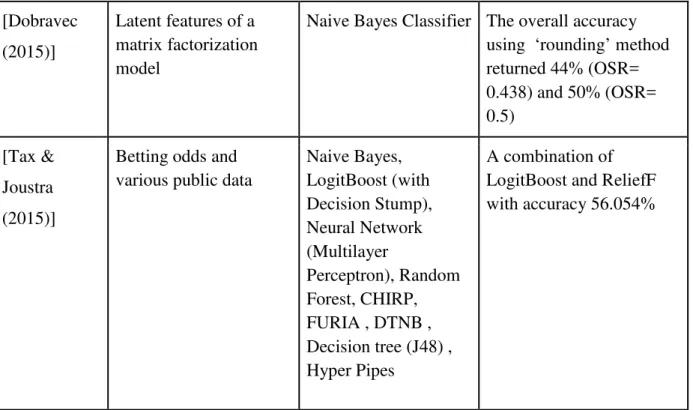
Prasetio and Harlili conducted a research to predict EPL season 2011/2012 matches by using all matches in EPL season 2010/2011 until 2015/2016 as training data. They used a logistic regression model to predict with accuracy result 69.5% [Prasetio (2016)]. Stefan Dobravec uses Naive Bayes Classifier as model and latent features obtained from matrix factorization process as features to create a goal score prediction model in order to predict the outcome of the FIFA World Cup 2014. The overall accuracy using ‘rounding’ method returned 44% (OSR= 0.438) and 50% (OSR= 0.5) using Naive Bayes classifier [Dobravec (2015)].
Tax and Joustra build a prediction system to predict the FTR results of soccer matches in Eredivisie, the highest competition of professional soccer in the Netherlands. They have investigated the impact of the match based features by comparing a model with betting odds and a hybrid model of both betting odds and match based features. They use machine learning software called WEKA to experiment with 9 classification algorithms. According to their research, the highest performing classification algorithms are Naive Bayes with a 3- component PCA, and the ANN with a 3 or 7- component PCA which have achieved an accuracy of 54.7%. [Tax & Joustra (2015)].
Although lots of research has been done in this field, to our knowledge, there is no previous research that using weather condition as a feature on machine learning to predict soccer outcome. Most of those previous researches also only focus on predict FTR result. This research will use two different kind of weather data which are average temperature (ºC), and Daily Total Precipitation (mm), this research also not only predict FTR but also whether the match end with more than 2 goals or not(over/under 2.5 goals). Table 2.2 show the list of all previous works.
Author Features Models Results
[Joseph et al. (2006)]
The quality of the opponent, presence of of 3 important players, match location, and the playing position of key player. Expert Bayesian Network (BN) compare with MC4, Naive BN, Hugun BN, and KNN
Expert BN has better overall accuracy with 59.21%
[Esme & Team’s brand value,
market value of team’s
K-Nearest Neighbors (KNN)
57.52% accuracy for FTR (k=18) and 86.27%
Kiran (2018)]
players, Standard deviation and probability based on fixed odds, the
frequency percentage of the betting odds, etc.
accuracy for Double Chance (k=5)
[Constantino u et al. (2012)]
Team strength, Team form, Psychological impact, Fatigue,
Bayesian network The model successfully
gain profit when used to bet on bookmakers [Yezus (2014)] Form, Concentration, Motivation, Goal difference, Score difference, History. K-Nearest Neighbors (KNN) and Random Forest Accuracy using Knn is 55.8% while Random Forest 63.4% [Sujatha et al. (2018)] UEFA coefficient, Home advantage , League rank, amount of Transfer money, number of goals scored and conceded, Wins and losses, League points, and cost of the team
Artificial Neural Network
In the case of predicting the winner, the model RMS error is more than FRES but it is less than FRES when it comes to predicting goals.
[Petterson & Nyquist (2017)]
Lineups, position, goal, card, substitution, and penalty
LSTM neural network The accuracy is between 33-45% (depends on architecture) when the match at 0th minute and between 73-86% when the match already pass 90th minute.
[Danisik et al. (2018)]
Players stats and match history
LSTM classification and regression models
The best accuracy is 52.479% from LSTM regression model [Prasetio
(2016)]
Home Offense, Away Offense, Home Defense, and Away Defense.
[Dobravec (2015)]
Latent features of a matrix factorization model
Naive Bayes Classifier The overall accuracy using ‘rounding’ method returned 44% (OSR= 0.438) and 50% (OSR= 0.5) [Tax & Joustra (2015)]
Betting odds and various public data
Naive Bayes, LogitBoost (with Decision Stump), Neural Network (Multilayer Perceptron), Random Forest, CHIRP, FURIA , DTNB , Decision tree (J48) , Hyper Pipes A combination of LogitBoost and ReliefF with accuracy 56.054%
3.
METHODOLOGY
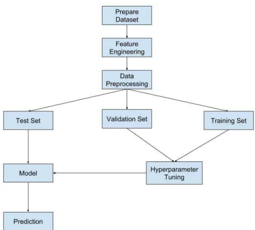
This chapter discusses every steps of the research implementation which include hardware and software, data gathering and preprocessing, create and select features that will be used for the models and develop the models. Figure 3.1 is the flowchart to visualize the methodology of this thesis.
Figure 3.1: Flowchart to visualize the methodology of the thesis
3.1.
Hardware and Software
Table 3.1 is list of all software used and Table 3.2 is the computer specification used for training the model. Python is chosen as programming language for this thesis because it has many options of inbuilt libraries that very useful for scientific computing. In this project, we used various libraries such as pandas for data manipulation and analysis, and seaborn for data visualization. phpMyAdmin also used to manipulate the dataset especially when created all necessary features. As for machine learning library, scikit-learn was used because it features various machine scikit-learning algorithms.
Programming Language Python version 3.6.6.
Database Administrator Tool phpMyAdmin version 4.8.4.
Integrated Development Environment Jupyter Notebook version 4.4.0.
Data Manipulation Pandas version 0.23.4.
Machine Learning Library Scikit Learn version 0.20.2.
Table 3.1: All software used during the thesis project.
CPU Intel(R) Core(TM) i7-7500 2.90 GHz
Motherboard Asus UX530UX
RAM 8 GB DDR4
Table 3.2: The computer specifications used for training the model.
3.2.
Data Sources
The historical matches dataset retrieved from football-data.co.uk contains matches of La Liga and Segunda division (also known as La Liga 2) from season 2013/2014 until 2016/2017. La Liga is men’s top professional soccer competition in spanish soccer league system, while Segunda division is 2nd behind La Liga. Every season since 2010-2011, top two teams and the play-off winner between teams rank 3rd - 6th promoted to La Liga for the next season replacing three lowest rank teams, this means every season the composition of teams played in La Liga and Segunda division always different from previous season.
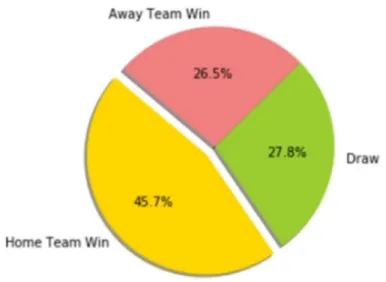
Totally there are 3830 matches from season 2013-2014 until 2016-2017, however for this thesis not all matches included in the final dataset since only matches with complete weather information will be eligible. In the end, only 3335 matches are eligible for final dataset. Figure 3.2 show the FTR distribution of the dataset and figure 3.3 show the over/under 2.5 goals distribution of the dataset.
Figure 3.2: Pie chart to visualize the distribution of FTR of the dataset
Figure 3.3: Pie chart to visualize the distribution of over/under 2.5 goals of the dataset
The weather dataset is from the Agencia Estatal de Meteorología(AEMT). The data format is in csv file and it has the temperature and rain information from 832 weather stations all across Spain. Below are the list of fields of AEMT csv files.
● Station Identifier ● Date
● Maximum Temperature (ºC) ● Maximum Temperature Hour ● Minimum temperature (ºC) ● Minimum Temperature Hour ● Average Temperature (ºC) ● Maximum wind streak (Km / h)
● Maximum Time of Streak ● Average Wind Speed (Km / h) ● Maximum Wind Speed Time ● Daily Total Precipitation (mm) ● Precipitation from 0 to 6 hours (mm) ● Precipitation from 6 to 12 hours (mm) ● Precipitation from 12 to 18 hours (mm) ● Precipitation from 18 to 24 hours (mm)
For this thesis, only daily total precipitation and average temperature are used in the ML models. AEMT also provide the ID of all stations complete with exact detail location, this information is useful to find the nearest weather station from each stadium. Figure show the screenshot of AEMT csv file.
Figure 3.4: The screenshot of AEMT csv file.
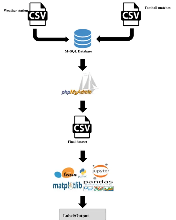
The way to find the exact weather situation for every matchday is by get the longitude and latitude of every team stadium from google map and then calculate the distance of every stadiums to every weather stations to find the closest weather station for each stadium using google sheet formula. After that, join both datasets based on weather station ID and the date of matchdays.
The join process happen in MySQL database since it is easy to do all data manipulation task using SQL query. Both csv files of spanish football matches and weather stations are converted into MySQL table and accessed using phpMyAdmin. Beside joining tables, SQL query also used to calculate total number of points gained and goal difference of each team in the last 4 home/away matches. The final dataset which consist of matches with complete weather information then reconverted into csv files, the final data then normalized and split into training/validation to train the model and
test dataset to check the capability of the model. Figure 3.5 show the process from raw data into classification result.
Figure 3.5: The process from raw data into classification result
3.3.
Features and Labels
Machine learning classification algorithms basically try to map input to an output based on correct input-output pairs of the unseen data [Russell & Norvig (2016)]. Before the model able to make prediction, it has to be “trained” with a correct input-output pairs
Weather station Football matches
MySQL Database
Label/Output
dataset, this step called the training phase. In this case, the input(features) consists of weather information and other soccer statistics from the match while the output(labels) is the outcome of the match that the model try to predict.
For this research, the label is the final outcome of the match (home team win, draw, or away team win) and over/under 2.5 goals. Set of features are divided into two groups: historic and weather. Table 3.3 is list of historic features with description and table 3.4 is list of weather features with description.
Name of Features Description
HTP4M The total points of home team in the last 4 home matches
ATP4M The total points of away team in the last 4 away matches
HTGOALDIFF The difference between number of goal scored and
conceded of the home team in the last 4 home matches.
ATGOALDIFF The difference between number of goal scored and
conceded of the away team in the last 4 away matches. Table 3.3: List of historic features with description.
Name of Features Description
TMED_DIFF Temperature difference between home and and away team
location
TPREC_HOME Total rain precipitation on the matchday
Table 3.4: List of weather features with description.
Historic features are the historical statistic for each team and do not depend on the rival while weather features represent the weather condition. The way of calculating the value of feature TMED_DIFF is by finding the difference between the temperature on the match location with the average temperature in the city of away team of in the last 6 days
Since not every city has complete information of the temperature, therefore we decide to only include matches where the temperature in the match location is not empty or 0 and the away team have temperature data at least 4 days in the last 6 days before the matchday. For example, if the away team have a match on Sunday but in the last 6 days
(Monday-Saturday) it only have weather information on Saturday, Friday, Tuesday, and Monday, therefore average temperature on those days will be added up and divide by 4 instead of 6.
3.4.
Data Preprocessing
Data preprocessing process is very essential to make sure the data is in a good quality to be used for machine learning algorithm, a data with a lot of noise and irrelevant input can lead to misleading results when predicting unseen data. This step requires a lot of time since it involves not only cleaning and normalizing the data but also transforming and extracting feature.
Some machine learning algorithm can really be affected by the different scale of the features. For example, KNN classifier tries to measure the distance between data points when trying to predict the label, this means features on large scale will dominate the prediction. To solve this issue, features need to be re-scaled as an initial step. All features used for this thesis are normalized, so the original value converted into number between 0 and 1.
3.5.
Data Splitting and K-Fold Cross-Validation
There are many ways to split the dataset, but due to the fact that there is a time-element in the professional soccer dataset then it is better to split data between training and testing historically. Table 3.5 show the overview of how the data is partitioned.
Season
Training/Validation 2013-2014
2014-2015 2015-2016
Test 2016-2017
Table 3.5: Overview of how the data is partitioned.
After performing the training process, the final model should be able to predict the label/output of testing dataset correctly, but most of the time the final model learn the detail and noise in the training data too well which make the model just memorizes the
training dataset so it unable give correct prediction to the pattern that was not in the training dataset, this problem called overfitting [Reitermanova (2010)].
One of the solutions to avoid overfitting is to implement k-fold cross-validation. The way it works is by separate the data into K parts of the same size. The Kth part of the dataset is used for validation and the rest of the dataset used to train the model, In most cases k = 10 is chosen which mean this process is repeated 10th times for each part of the data. This process able to reduce the risk of overfitting because for each iteration the final model is using a different combination of training and validation dataset. Figure 3.6 show K-fold cross-validation visualization with k=10
.
Figure 3.6: K-fold cross-validation visualization with k=10
3.6.
Hyperparameter Optimization
Beside data splitting, another factor besides that need to be considered to find the best algorithm is the choice of parameters values, or famously known as hyperparameter optimization. Every algorithm has different hyperparameters, for example in KNN algorithm it will be the value of K while for SVN it will be the type of kernel.
Usually, the value of hyperparameters is choosing randomly and then pick the hyperparameters value with the best accuracy result. But it can be a very exhausting process especially there is more than one hyperparameter for each algorithm, therefore it is better to use an algorithm to find the best hyperparameter combination automatically such as grid-search.
By using scikit-learn library, Grid Search algorithm can be implemented by importing a class called GridSearchCV. The first step to do after importing the class is to create a
list of parameters and their possible values for the algorithm. Table 3.6 show the dictionary of parameters and their possible values for KNN, SVM, and RF algorithms.
Algorithm Hyperparameters Value
KNN Neighbors Numbers between 3 to 50
Weight ['uniform','distance'] Metric ['manhattan','minkowski','euclidean'] SVM Kernel ['linear', 'rbf'] Gamma [0.1, 1, 10, 100 ,500, 1000] C [0.1, 1, 10, 100 ,500, 1000] RF Estimators [10,50,100,150,200]
Minimum Samples Leaf [1,5,10,50,100,200,500]
Maximum Features ['auto', 'sqrt', 'log2']
Table 3.6: The list of parameters and their values for KNN, SVM, and RF algorithms.
The way grid Search algorithm work is by execute all possible combinations of parameter values and after that choose the combination with the best accuracy score. For example, to find the best combination between the value of k (1 to 50), weight (uniform or distance), and metric (manhattan, minkowski, or euclidean) for KNN algorithm then it will check 300 combinations (50 x 2 x 3 = 300).
The next step after creating a parameter dictionary is to pass the algorithm, parameters dictionary, and the number of folds for cross for cross-validation to . And the last step is to call fit method and pass the training/validation dataset. The algorithm will be executed 3000 times since there are 10-fold cross validation and 300 combinations of parameters (300x10 = 3000).
This process definitely takes a lot of time. But even though the grid-search process takes a lot of time, it is pretty straightforward and safer compare to other methods which avoid doing an exhaustive parameter search [Hsu et al. (2003)].
4.
EVALUATION
This chapter shows the prediction result using chosen algorithms. In order to see how temperature difference and rain precipitation can affect the prediction accuracy, the dataset will divide into two part for each category(Rain and temperature). The weather category divide the dataset based on the value of temperature different feature where one part will be matches with temperature difference below 5° and another one with temperature difference above 5°. The rain category divide the dataset based on the value of rain precipitation feature where one part will be matches with rain precipitation below 5 mm and another one with rain precipitation above 5 mm.
4.1.
Dataset and Features
In order to really understand the impact of the weather into soccer outcome, we decide to split dataset based on temperature difference (TMED_DIFF) and rain precipitation (TPREC_HOME). The dataset is split into two dataset between temperature difference below 5° and above 5° because the assumption is matches with extreme temperature difference will increase the accuracy of prediction. Table 4.1 show total number of matches for datasets with temperature difference below and above 5°. It is not surprise that number of data points are unequal since most of cities in Spain having similar climate. The average temperature difference of every match is 4.41°.
Temperature Difference Dataset Data Points
Below 5° Training/Validation 1578
Test 567
Above 5° Training/Validation 773
Test 208
Table 4.1: Number of matches for dataset with temperature difference below and above 5°
Next is to split the dataset based on rain precipitation. The dataset is split into two dataset between rain precipitation below 5 mm and above 5 mm because the assumption
is matches with high rain precipitation will decrease the number of goals. Table 4.2 show total number of matches for datasets with rain precipitation below and above 5 mm.
Rain Precipitation Dataset Data Points
Below 5 mm Training/Validation 2149
Test 702
Above 5 mm Training/Validation 226
Test 77
Table 4.2: Number of matches for dataset with rain precipitation below and above 5 mm.
Beside split the dataset based on temperature difference and rain precipitation, the data also split into two different case study based on features used, case study 1 only use weather features while case study 2 use both weather and historical statistics features. Table 4.3 show the list of features for both case studies.
Case study 1 and 2 TMED_DIFF
TPRE_HOME
Case study 2 HTP4M
ATP4M
HYGOALDIFF
ATGOALDIFF
Table 4.3: List of features for case study 1 and 2
specifically for features HT4M and ATP4M, both are not applicable to predict over/under 2.5 goals since both are total accumulated point from previous home/away matches which have no correlation with number of goals.
4.2.
Best Hyperparameters
Table 4.4, 4.5 and 4.6 show the result of hyperparameter optimization of each algorithm for matches above and below 5° temperature difference and table 4.7, 4.8 and 4.9 show the result of hyperparameter optimization of each algorithm for matches above and below 5 mm rain precipitation. The best hyperparameters value is determined by Grid Search method join with 5-Fold Cross-Validation. The best hyperparameters value combination are picked based on the accuracy score.
Dataset Features Hyperparameters Best Value
Below 5° Case study 1 Metric Manhattan
Neighbors 11
Weight Distance
Case study 2 Metric Manhattan
Neighbors 26
Weight Distance
Above 5° Case study 1 Metric Manhattan
Neighbors 3
Weight Distance
Case study 2 Metric Manhattan
Neighbors 12
Weight Distance
Table 4.4: Result of hyperparameter optimization of KNN model for matches above and below 5° temperature difference
Below 5° Case study 1 C 100 Gamma 10 Kernel RBF Case study 2 C 1 Gamma 500 Kernel rbf
Above 5° Case study 1 C 500
Gamma 1000
Kernel rbf
Case study 2 C 1
Gamma 500
Kernel rbf
Table 4.5: Result of hyperparameter optimization of SVM model for matches above and below 5° temperature difference
Dataset Features Hyperparameters Best Value
Below 5° Case study 1 Estimators 50
Maximum Features log2 Minimum Samples Leaf 1
Case study 2 Estimators 150
Maximum Features
min_samples_leaf 1
Above 5° Case study 1 estimators 100
Maximum Features Auto Minimum Samples Leaf 1
Case study 2 estimators 100
Maximum Features sqrt Minimum Samples Leaf 1
Table 4.6: Result of hyperparameter optimization of RF model for matches above and below 5° temperature difference
Dataset Features Hyperparameters Best Value
Below 5 mm Case study 1 Metric Manhattan
Neighbors 8
Weight Distance
Case study 2 Metric Minkowski
Neighbors 9
Weight Distance
Above 5 mm Case study 1 Metric Manhattan
Neighbors 45
Weight Distance
Neighbors 47
Weight Distance
Table 4.7: Result of hyperparameter optimization of KNN model for matches above and below 5 mm rain precipitation.
Dataset Features Hyperparameters Best Value
Below 5 mm Case study 1 C 100
Gamma 10
Kernel RBF
Case study 2 C 500
Gamma 500
Kernel rbf
Above 5 mm Case study 1 C 10
Gamma 100
Kernel rbf
Case study 2 C 10
Gamma 100
Kernel rbf
Table 4.8: Result of hyperparameter optimization of SVM model for matches above and below 5 mm rain precipitation.
Dataset Features Hyperparameters Best Value
Below 5 mm Case study 1 Estimators 10
Maximum Features sqrt Minimum Samples Leaf 1
Case study 2 Estimators 50
Maximum Features
sqrt
min_samples_leaf 1
Above 5 mm Case study 1 estimators 100
Maximum Features Auto Minimum Samples Leaf 1
Case study 2 estimators 150
Maximum Features auto Minimum Samples Leaf 1
Table 4.9: Result of hyperparameter optimization of RF model for matches above and below 5 mm rain precipitation.
4.3.
Confusion Matrix
Figure 4.1 is the confusion matrices of FTR prediction and figure 4.2 is the confusion matrices of over/under 2.5 goals prediction. Cells with black background show the number of samples correctly predicted.
Figure 4.1: Confusion Matrices of FTR prediction using KNN, SVM, and RF models.
b) Case study 2
Figure 4.2: Confusion Matrices of over/under 2.5 goals prediction using KNN, SVM, and RF models
4.4.
Model Accuracy
Table 4.10 show the accuracy score of FTR prediction and table 4.11 show the accuracy score of over/under 2.5 goals prediction using KNN, SVM, and RF algorithms. As said before on chapter 2, the way to calculate the accuracy is by sum total number of samples correctly predicted divided by total number of samples in dataset.
Features KNN(%) SVM(%) RF(%)
Below 5° Above 5° Below 5° Above 5° Below 5° Above 5°
Case study 1 42.68 47.11 44.79 47.59 43.73 46.63
Case study 2 43.38 41.82 45.32 49.51 41.62 43.26
Figure 4.3: Bar chart to visualize accuracy of each model for FTR prediction.
For FTR prediction, In the experiment where only TMED_DIFF and TPREC_HOME used as features (case study 1), all models showing better accuracy score for dataset with temperature difference above 5° compare to below 5°. SVM model show the best accuracy with 47.59% but KNN is better in terms of accuracy improvement from below 5° to above 5°. KNN model show the best improvement of accuracy (4.43%), followed by RF (2.9%), and SVM (2.8%). In the experiment where all features are used to predict surprisingly SVM is the only model to show improvement of accuracy prediction for both below and above 5°, this results are unexpected since it was assume that by adding historical statistics as features it will improve the prediction accuracy for every model. KNN model is even show decrease of accuracy prediction from below 5° to above 5° (-1.56%), SVM accuracy for dataset above 5° is 49.51% which is an improvement of 4.19% compare to dataset below 5°.
Features KNN(%) SVM(%) RF(%) Below 5 mm Above 5 mm Below 5 mm Above 5 mm Below 5 mm Above 5 mm Case study 1 47.35 49.33 53.07 53.33 52.78 54.66 Case study 2 47.78 53.33 51.21 56 51.78 54.66
Table 4.11: Proportion of over/under 2.5 goals correctly predicted for each model.
Figure 4.4: Bar chart to visualize accuracy of each model for over/under 2.5 goals prediction.
For over/under 2.5 goals, every models show the increase of accuracy from rain precipitation below 5 mm to above 5 mm. In case study 1 where only rain and temperature difference used as features, KNN show the best improvement from 47.35% to 49.33% (+1.98%) followed by RF(+1.88%) and SVM (+0.25%). In case study 2, KNN show the best improvement(+5.58%) followed by SVM(+4.79%) and RF(+2.28%). KNN also show better accuracy in case study 2 compare to case study 1. Overall, the best accuracy is coming from SVM in case study 2 with 56%.
4.5.
Misclassification Rate
Choose the best model based solely on accuracy score can be misleading because in many situations where the dataset have large class imbalance, a model can predict the value of the majority class for every predictions and achieve a high classification accuracy. Chapter 3 is show the class distribution of the dataset where most of the times home team win the match. So in order to find an ideal model, misclassification rate also need to be calculated. Table 4.12 show the misclassification rate for FTR classes and table 4.13 show the misclassification rate for over/under 2.5 goals classes.
Models Labels
Case study 1 Case study 2
Below 5° Above 5° Below 5° Above 5°
KNN Home Team Win 15.44 11.76 23.93 30.39
Draw 94.51 88.88 85.97 83.33
Away Team Win 90.27 96.15 81.94 86.53
SVM Home Team Win 3.86 9.8 3.86 0.98
Draw 100 94.44 85.97 96.29
Away Team Win 96.52 92.30 81.94 100
Draw 95.12 88.88 80.48 83.33
Away Team Win 88.88 94.23 79.16 78.84
Table 4.12: Misclassification rate of FTR prediction for each models
It can be observed from the results of classification shown in Table 4.12 that SVM classifier gives the best performance in terms of classification accuracy but it also gives high misclassification rate on both draw and away team win. Further, in one case SVM classifiers even show 100% misclassification rate on away team win class: which mean it failed to predict every sample in that class. Based on solely on misclassification rate, we can say that RF model is more balance since only two times it has class with more than 90% misclassification rate.
Models Labels
Case study 1 Case study 2
Below 5 mm Above 5 mm Below 5 mm Above 5 mm KNN Below 2.5 87.43 42.85 54.81 9.52 Over 2.5 12.61 60.60 49.23 93.93 SVM Below 2.5 5.61 11.90 31.28 33.33 Over 2.5 94.46 90.90 68.92 57.57 RF Below 2.5 9.09 45.23 30.74 33.33 Over 2.5 91.02 45.45 68.30 60.60
Table 4.13: Misclassification rate of over/under 2.5 for each models
From table 4.13 we can see that SVM have class with more than 90% misclassification rate on both below and above 5 mm rain precipitation on case study 1, It is prove that
the training process of the model is not very well since it predict the same class most of the times. Same thing can be said for RF when predict the label using dataset below 5 mm (case study 1) and KNN when predict the label using dataset above 5 mm (case study 2).
4.6.
Comparison with betting odds
Bookmarker always put the lowest odds to the most likely outcome according to them. Table 4.14 show the percentage of correct prediction from Bet365 and Betbrain.
FTR Over/Under 2.5
Correct Prediction Temperature
difference above 5°
52.88% Rain Precipitation
above 5 mm
69.33%
Incorrect Prediction 47.11% 30.66%
Correct Prediction Temperature
difference below 5°
50.08% Rain Precipitation
below 5 mm
60.51%
Incorrect Prediction 49.91% 39.48%
Table 4.14: Prediction accuracy of bookmarkers.
Unfortunately there is no model from this thesis that have better accuracy than those two bookmarkers. The accuracy of Bet365 on predicting FTR for dataset with temperature difference above 5° is 52.88% (compare to SVM with 49.51%) and for dataset with temperature difference below 5° is 50.08% (compare to SVM with 45.32%). The accuracy of Betbrain on predicting over/under 2.5 goals for dataset with rain precipitation above 5 mm is 69.33% (compare to SVM with 56%) and for dataset with rain precipitation below 5 mm is 60.51% (compare to SVM with 53.07%).
5.
CONCLUSION
Weather condition show a good potential to improve predictions of the outcome of soccer games. In case of FTR prediction, SVM show better result with 44.79% for matches with temperature difference below 5° and 47.59% for temperature difference above 5°, When other historical statistics features also used the accuracy rate improve significantly with 45.32% for temperature difference below 5° and 49.51% for temperature difference above 5°. In case of over/under 2.5 goals prediction, SVM show 53.07% for rain precipitation below 5 mm but for rain precipitation above 5 mm RF has better result with 54.66%, When other historical statistics features also used SVM show better result than KNN and RF for both below and above 5 mm with 51.21% and 56%. However, the accuracy result of all models in this thesis is unable to beat bookmakers prediction. The misclassification rate calculation also show in many cases the model have more than 90% misclassification rate on certain class. There are many things that still can be done by the future research to improve this thesis; for example, other weather data could be used beside rain and temperature difference, the weather data during the exact timespan of the match also could improve the accuracy of the model, and more variation on dataset samples such as match between two team from different country or continent could also improve the accuracy since the temperature difference can be more significant, and since the final dataset is available in MySQL database, the future research can create REST hosted services with a underlying MySQL database so the ML model can do the prediction on real-time .
REFERENCES
Bunker, R. P., & Thabtah, F. (2017). A machine learning framework for sport result prediction. Applied Computing and Informatics.
Byrne, K. (2016). Coaches explain ideal weather conditions for a World Cup soccer match. https://www.accuweather.com/en/weather-news/how-does-weather-impact-the-sport-of-soccer/70005170. [Online; accessed 28-12-2018].
Constantinou, A. C., Fenton, N. E., & Neil, M. (2012). pi-football: A Bayesian network model for forecasting Association Football match outcomes. Knowledge-Based Systems, 36, 322-339.
Cortes, C., & Vapnik, V. (1995). Support-vector networks. Machine learning, 20(3), 273-297.
D. Petterson & R. Nyquist (2017). Football match prediction using deep learning Master’s thesis, Chalmers University of Technology.
Danisik, N., Lacko, P., & Farkas, M. (2018, August). Football Match Prediction Using Players Attributes. In 2018 World Symposium on Digital Intelligence for Systems and Machines (DISA) (pp. 201-206). IEEE.
Data School (2014). Simple guide to confusion matrix terminology.
https://www.dataschool.io/simple-guide-to-confusion-matrix-terminology/. [Online; accessed 28-12-2018].
Dobravec, S. (2015, May). Predicting sports results using latent features: A case study. In Information and Communication Technology, Electronics and Microelectronics (MIPRO), 2015 38th International Convention on (pp. 1267-1272). IEEE.
Esme, E., & Kiran, M. S. (2018). Prediction of Football Match Outcomes Based on Bookmaker Odds by Using k-Nearest Neighbor Algorithm. International Journal of Machine Learning and Computing, 8(1).
FIFA (2018). Laws of the Game. https://resources.fifa.com/image/upload/Laws-of-The-game-2018-19.pdf?cloudid=khhloe2xoigyna8juxw3. [Online; accessed 28-12-2018].
FIFA (2018). More than half the world watched record-breaking 2018 World Cup.
https://resources.fifa.com/image/upload/2018-fifa-world-cup-russia-global-broadcast-and-audience-executive-summary.pdf?cloudid=njqsntrvdvqv8ho1dag5. [Online; accessed 28-12-2018].
Hsu, C. W., Chang, C. C., & Lin, C. J. (2003). A practical guide to support vector classification.
James, G., Witten, D., Hastie, T., & Tibshirani, R. (2013). An introduction to statistical learning (Vol. 112). New York: springer.
Joseph, A., Fenton, N. E., & Neil, M. (2006). Predicting football results using Bayesian nets and other machine learning techniques.Knowledge-Based Systems, 19(7), 544-553.
Karthikeyan, T., Ragavan, B., & Poornima, N. A comparative study of algorithms used for leukemia detection (2016). International Journal of Advanced Research in Computer Engineering & Technology (IJARCET) Volume, 5.
Keogh, F. & Rose, G. (2013). Football betting - the global gambling industry worth billions. https://www.bbc.com/sport/football/24354124. [Online; accessed 28-12-2018].
Kurama, V. (2018). Unsupervised Learning with Python.
https://towardsdatascience.com/unsupervised-learning-with-python-173c51dc7f03. [Online; accessed 28-12-2018].
Mitchell, T. M. (1997). Machine learning (mcgraw-hill international editions computer science series).
Mulak, P., & Talhar, N. (2015). Analysis of Distance Measures Using K-Nearest Neighbor Algorithm on KDD Dataset. International Journal of Science and Research, 4(7), 2101-2104.
Online-Betting.me.uk (n.d.). Understanding betting odds to beat them.
https://www.online-betting.me.uk/articles/betting-odds-explained.php. [Online;
accessed 21-02-2019].
Prasetio, D. (2016, August). Predicting football match results with logistic regression. In Advanced Informatics: Concepts, Theory And Application (ICAICTA), 2016 International Conference On (pp. 1-5). IEEE.
Reitermanova, Z. (2010). Data splitting. In WDS (Vol. 10, pp. 31-36).
Russell, S. J., & Norvig, P. (2016). Artificial intelligence: a modern approach. Malaysia; Pearson Education Limited,.
Shalev-Shwartz, S., & Ben-David, S. (2014). Understanding machine learning: From theory to algorithms. Cambridge university press.
Sujatha, K., Godhavari, T., & Bhavani, N. P. (2018). Football Match Statistics Prediction using Artificial Neural Networks. International Journal of Mathematical and Computational Methods, 3.
Tax, N., & Joustra, Y. (2015). Predicting the Dutch football competition using public data: A machine learning approach. Transactions on Knowledge and Data Engineering, 10(10), 1-13.
Total Sportek (2016). 25 World's Most Popular Sports (Ranked by 13 factors). https://www.totalsportek.com/most-popular-sports/. [Online; accessed 28-12-2018].
Verikas, A., Gelzinis, A., & Bacauskiene, M. (2011). Mining data with random forests: A survey and results of new tests. Pattern recognition, 44(2), 330-349.
Vuk, M., & Curk, T. (2006). ROC curve, lift chart and calibration plot. Metodoloski zvezki, 3(1), 89.
Merriam-Webster (n.d.). Weather.
http://www.merriam-webster.com/dictionary/weather. [Online; accessed 28-12-2018].
Yezus, A. (2014). Predicting outcome of soccer matches using machine learning. Saint-Petersburg University.
Zipperman, M. A. (2014). Quantifying The Impact Of Temperature And Wind On NFL Passing And Rushing Performance.
ANNEX
● Query to calculate total number of points for each team in the last 4 home and away matches.
BEGIN
SET @matchday1 := 1; SET @matchday2 := 4;
while @matchday2 < matches do
UPDATE `FINAL_DATASET` as t1 INNER JOIN (SELECT MAX(RowHome)
as RowHome, IDDIVISION, IDSEASON, IDHOMETEAM, HOMETEAM, MAX(DATE) AS MaxDate,sum(HP) AS SumFTHP FROM `FINAL_DATASET` WHERE RowHome >= @matchday1 AND RowHome <=@matchday2 AND IDSEASON = idseasons AND IDDIVISION = iddivisions GROUP BY IDHOMETEAM) as t2 ON
t1.IDHOMETEAM = t2.IDHOMETEAM AND t1.RowHome = t2.RowHome+1 AND
t1.IDSEASON = t2.IDSEASON AND t1.IDDIVISION = t2.IDDIVISION
SET t1.HTP5M = t2.SumFTHP;
UPDATE `FINAL_DATASET` as t1 INNER JOIN (SELECT MAX(RowAway) as
RowAway, IDDIVISION, IDSEASON, IDAWAYTEAM, AWAYTEAM, MAX(DATE) AS MaxDate,sum(AP) AS SumFTAP FROM `FINAL_DATASET` WHERE RowAway >= @matchday1 AND RowAway <=@matchday2 AND IDSEASON = idseasons AND IDDIVISION = iddivisions GROUP BY IDAWAYTEAM) as t2 ON
t1.IDAWAYTEAM = t2.IDAWAYTEAM AND t1.RowAway = t2.RowAway+1 AND
t1.IDSEASON = t2.IDSEASON AND t1.IDDIVISION = t2.IDDIVISION
SET t1.ATP5M = t2.SumFTAP;
SET @matchday1 := @matchday1+1; SET @matchday2 := @matchday2+1; end while;
END
● Query to calculate number of goal scored and conceded for each team in the last 4 home and away matches
BEGIN
SET @matchday1 := 1;
SET @matchday2 := 4;
![Figure 2.1: RF architecture [Verikas et al. (2011)]](https://thumb-eu.123doks.com/thumbv2/123dok_br/15570702.1047983/15.892.230.682.130.376/figure-rf-architecture-verikas-et-al.webp)