Coupled modelling of the Tagus and Sado estuaries and their associated mesoscale patterns

(1)

Universidade de Aveiro 2015

Departamento de Física

Américo Soares Ribeiro

Coupled Modelling of the Tagus and Sado estuaries

and their Associated Mesoscale Patterns

Modelação Acoplada dos Estuários do Tejo e do

Sado e Padrões de Mesoescala Associados

(2)

(3)

Universidade de Aveiro 2015

Departamento de Física

Américo Soares Ribeiro

Coupled Modelling of the Tagus and Sado estuaries

and their Associated Mesoscale Patterns

Modelação Acoplada dos Estuários do Tejo e do

Sado e Padrões de Mesoescala Associados

Dissertação apresentada à Universidade de Aveiro para cumprimento dos requisitos necessários à obtenção do grau de Mestre em Ciências do Mar e das Zonas Costeiras, realizada sob a orientação científica do Doutor João Miguel Sequeira Silva Dias, Professor Auxiliar com Agregação do Departamento de Física da Universidade de Aveiro e co-orientação do Doutor João Daniel Alonso Antão Lencart e Silva, Bolseiro em gestão de Ciência e Tecnologia no Instituto Português do Mar e da Atmosfera (IPMA).

Este trabalho foi desenvolvido no âmbito do projeto BioChangeR (PTDC/AAC-AMB/121191/2010).

(4)

(5)

o júri

Presidente

_{Doutora Filomena Maria Cardoso Pedrosa Ferreira Martins}

Professora Associada do Departamento de Ambiente e Ordenamento da Universidade de Aveiro

Arguente

_{Doutora Magda Catarina Ferreira de Sousa}

Investigadora de Pós-Doutoramento do CESAM da Universidade de Aveiro

Orientador

_{Doutor João Miguel Sequeira Silva Dias}

(6)

(7)

acknowledgements I could not have accomplished this MSc thesis without the support and friendship of a great number of people.

To Prof. João Miguel Dias, who has been my supervisor since the beginning of my academic path and has been a great contributor to my development, both as person and as a researcher. It would not have been possible to complete my MSc degree without his suggestions and comments, and above all the important advices and friendship during the course of this work.

To João Daniel Lencart e Silva for the help during the Delft3D introduction, to solve several problems, also for the valuable suggestions, especially in the numerical model setup.

No word is big enough to express my gratitude to Magda C. Sousa, for being always there as a friend and dedicated “mentor”, who has given me an enormous and valuable help during my academic path.

To the NMEC (Estuarine and Coastal Modeling Group) for providing me all the conditions to keep carrying my work, namely Nuno Vaz, Renato Mendes, Ana Picado, Carina Lopes and João Rodrigues for the help and when needed the availability for the doubts.

To HIDROMOD, specially to João Ribeiro for providing the PCOMS data.

A special thanks to my friends André Pinto, Rita Longo and Vanessa Andreso, for sharing my frustrations, as well as my victories.

To my parents, Henrique and Filomena for their unconditional support I could always count on.

To all of them I owe the achievement of my MSc degree and to them I dedicate this thesis.

(8)

(9)

palavras-chave Dinâmica estuarina; Tejo; Sado; Delft3D; Traçador; Descarga; Pluma estuarina, Advecção.

resumo Dada a proximidade entre os estuários do Tejo e do Sado, é reconhecido que as descargas destes estuários ocorrem na mesma região costeira. O conhecimento atual relativo à hidrodinâmica dos estuários do Tejo e do Sado resulta maioritariamente da exploração de resultados de modelos numéricos, que descrevem as propriedades físicas e padrões gerados pelas correntes de maré e descargas fluviais. Não obstante, verificou-se que a interação entre estes dois sistemas não é considerada, não havendo esforços no sentido de estudar os dois sistemas simultaneamente, bem como de descrever as relações que partilham e identificar as mútuas influências a nível dinâmico. Com este objetivo, foi implementado o modelo numérico tridimensional Delft3D-Flow, de forma a investigar a dinâmica do estuário do Tejo, do Sado e da região costeira adjacente. O modelo numérico foi calibrado e validado com a altura de maré, correntes, salinidade e temperatura da água, sendo aplicado para a investigação do efeito das descargas fluviais e do efeito do vento na interação das plumas destes estuários. O período escolhido para as simulações foi o Inverno de 2009-2010. Foram impostos dois tipos de forçamentos na fronteira aberta oceânica, um que comtempla as correntes de mesoescala e outro apenas a dinâmica costeira. Foram considerados cinco cenários para ventos moderados nos quatro principais quadrantes e para a ausência deste. Através do uso de dois traçadores distintos, foram escolhidos três cenários idealizados com descargas baixas, moderadas e altas dos rios Tejo e Sado.

Os resultados evidenciaram a presença de plumas estuarinas, filamentos e eddies causados pela interação entre os estuários e a região costeira. Os resultados obtidos revelam ainda uma intrusão da pluma estuarina do Sado no estuário do Tejo após descargas fluviais significativas durante dez dias, contudo, este padrão não foi observado na pluma estuarina do Tejo. Foi ainda observado que a água estuarina do Sado se propaga para o estuário do Tejo em apenas 36 horas com apenas a dinâmica costeira, ao passo que com as correntes de mesoescala só se observou a intrusão após 120 horas.

Sumariamente, o modelo desenvolvido para este estudo contribuiu para a caracterização e compreensão da interação entre os estuários do Tejo e Sado, e definição das condições em que esta ocorre.

(10)

(11)

keywords Estuarine dynamics; Tagus; Sado; Delft3D; Tracer; freshwater flow; Estuarine plume; Advection.

abstract Given the close proximity between the Tagus and Sado estuaries, it is understandable that these two hydrodynamic systems have their discharges on the same coastal region. Several studies focus on the investigation of the complex circulation at the mouth of Tagus or Sado estuaries, however, the interaction between these two systems is not taken into account and there are no studies which contemplate the interaction between the two estuaries. With this objective, the three-dimensional model Delft3D-Flow was implemented in order to investigate the complex flows in Tagus and Sado estuaries and adjacent shelf. The numerical model was calibrated and validated using sea surface height, currents, salinity and water temperature data, and then applied to research the role of river discharge and wind effects under mesoscale currents and coastal dynamics at open ocean boundaries on the plumes interaction. The chosen period was the winter of 2009-2010. To examine the response of the estuarine plumes to different wind directions, five scenarios of moderate winds were considered blowing from each of the main four compass points, and with the absence of wind. Through the use of two distinct tracers, three different idealized scenarios were chosen: low, moderate and high Tagus and Sado river discharges.

The results showed an evidence of estuarine plumes, filaments and mesoscale eddies caused by the interactions between the estuaries and the nearby coastal region. The obtained results also reveal a intrusion caused by the Sado plume in Tagus estuary after a 10-day simulation. This pattern was not observed for Tagus plume. It was also observed that the Sado estuarine water propagates to Tagus estuary in just 36 hours with coastal dynamics, when compared to the mesoscale currents forcing took around 120 hours.

In summary, the model application developed in this study contributed to the characterization and understanding of the interaction between Tagus and Sado estuary’s, and in which conditions these occur.

(12)

(13)

Contents|xi

List of Figures

Figure 2.1: Study area: Geography of the Western Iberian System, showing the main features referred

in the text. 10

Figure 2.2: Location and bathymetry of Tagus estuary and the three freshwater inflows: Tagus river,

Sorraia river and Vale Michões tributary. 11

Figure 2.3: Tagus River basin location. 12

Figure 2.4: Location and bathymetry of Sado estuary and the two freshwater flows: Sado River and

Marateca tributary. 13

Figure 2.5: Sado River: Basin location; Mean annual flow. 15

Figure 2.6: The eastern North Atlantic region. Principal currents in the eastern North Atlantic. 17 Figure 3.1: Numerical grid and the location of the tide gauge, water temperature and salinity stations

used in the model calibration. 20

Figure 3.2: Local wind for the study area: wind vector for the period of 2009 and 2012. 22

Figure 4.2: Example of σ and Z-grid. 26

Figure 4.1: Numerical grid and the location of the tide gauge, water temperature and salinity stations

used in the model calibration. 26

Figure 5.2: Study area numerical bathymetry. 38

Figure 5.1: Horizontal grid: multi-domain and single-domain. 38

Figure 5.3: Location of the stations used for visual comparison between the observed and predicted

water levels. 42

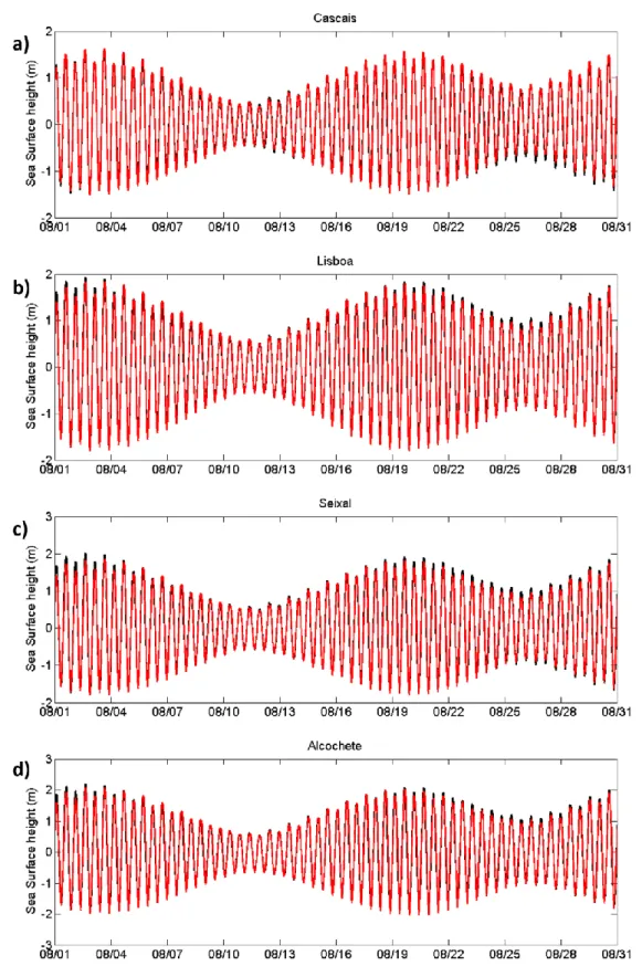
Figure 5.4: Comparison between predicted and observed sea surface height for Tagus: Cascais;

Lisboa; Seixal and Alcochete stations. 43

Figure 5.5: Comparison between predicted and observed sea surface height for Sado: Baliza; Tróia;

Desmagnetização and Setenave stations. 44

Figure 5.6: Harmonic comparison for the 20 tidal stations spatially distributed in the Tagus and Sado

estuaries. 47

Figure 5.7: Horizontal velocities: RMSE values for u and v direction, and skill values for u and v

direction. 48

Figure 5.8: Observations and predictions for salinity vertical profiles for the sampling stations P10 and

P12. 49

Figure 6.1: Monthly mean of Tagus and Sado discharge. Probability distributions for Tagus and Sado

discharge. 52

Figure 6.2: Mask applied to the grid area to calculate the propagation of the estuary plume of Tagus and Sado. Cross-section to measure the advected tracer from Tagus estuary and Sado estuary. 54 Figure 7.1: Initial instant for Tagus and Sado in all scenarios, for all the layers. Cross-section to

measure the advected tracer from Tagus estuary and Sado estuary. 58

Figure 7.2: Tagus scenarios after 10 days for the surface layer and bottom layer, under high river discharges of 0.95 non-exceedance probability for mesoscale currents. 59 Figure 7.3: Sado scenarios after 10 days for the surface layer and bottom layer, under high river

discharges of 0.95 non-exceedance probability for mesoscale currents. 60 Figure 7.4: Cumulative advective transport of Sado tracer in Cross-section II and Tagus tracer in

(16)

xiv| List of Figures

Figure 7.5: Tagus scenarios after 10 days for the surface layer and bottom layer, under moderate river discharges of 0.80 non-exceedance probability for mesoscale currents. 63 Figure 7.6: Sado scenarios after 10 days for the surface layer and bottom layer, under moderate river

discharges of 0.80 non-exceedance probability for mesoscale currents. 64 Figure 7.7: Tagus scenarios after 10 days for the surface layer and bottom layer, under low river

discharges of 0.50 non-exceedance probability for mesoscale currents. 66 Figure 7.8: Sado scenarios after 10 days for the surface layer and bottom layer, under low river

discharges of 0.50 non-exceedance probability for mesoscale currents. 67 Figure 7.9: Tagus scenarios after 10 days for the surface layer and bottom layer, under high river

discharges of 0.95 non-exceedance probability for coastal dynamics. 69 Figure 7.10: Sado scenarios after 10 days for the surface layer and bottom layer, under high river

discharges of 0.95 non-exceedance probability for coastal dynamics. 70 Figure 7.11: Cumulative advective transport of Sado tracer in Cross-section II and Tagus tracer in

Cross-section I. 71

Figure 7.12: Tagus scenarios after 10 days for the surface layer and bottom layer, under moderate river discharges of 0.80 non-exceedance probability for coastal dynamics. 72 Figure 7.13: Sado scenarios after 10 days for the surface layer and bottom layer, under moderate river discharges of 0.80 non-exceedance probability for coastal dynamics. 73 Figure 7.14: Tagus scenarios after 10 days for the surface layer and bottom layer, under low river

discharges of 0.50 non-exceedance probability for coastal dynamics. 75 Figure 7.15: Sado scenarios after 10 days for the surface layer and bottom layer, under low river

discharges of 0.50 non-exceedance probability for coastal dynamics. 76 Figure 7.16: Vertical profile of cumulative advective transport of Tagus tracer and Sado tracer in

Cross-section II, for 240 h after the simulation start. 79

Figure 7.17: Tagus scenarios for the 10-day simulation under discharges of 0.95, 0.80 and 0.50 non-exceedance probability for the surface layer, with Riemann forcing. 81 Figure 7.18: Sado scenarios for the 10-day simulation under discharges of 0.95, 0.80 and 0.50

non-exceedance probability for the surface layer, with Riemann forcing. 82 Figure 7.19: Tagus scenarios for the 10-day simulation under discharges of 0.95, 0.80 and 0.50

non-exceedance probability for the surface layer, with Harmonic forcing. 84 Figure 7.20: Sado scenarios for the 10-day simulation under discharges of 0.95, 0.80 and 0.50

(17)

List of Tables |xv

List of Tables

Table 3.1: Sample Stations for water level. 21

Table 3.2: Sample Stations for salinity and temperature. 21

Table 5.1: Percentage of Depth per layer, with layer 1 representing the surface and layer 15 the

bottom. 39

Table 5.2: Bottom friction coefficients. 40

Table 5.3: Error values for tidal water levels. 45

Table 6.1: Modelling configuration for the study area. 51

Table 6.2: Non exceedance Probability (NEP). 53

(18)

(19)

Introduction|1

1. Introduction

1.1. Background and motivation

For centuries, estuaries have been regions of extremely high importance to human kind. These regions are characterized by their high productivity due to river discharges, through their role as nurseries for several animal species and by providing sheltered anchorages and easy navigational access to the ocean.

Here, small and large-scale mixing processes act to produce high mixing rates and spatially inhomogeneous concentration distributions, namely the river plumes. The river plumes have higher concentration of nutrients than the ocean waters, affecting the biomass accumulation and productivity in the plume-influenced region, leading to a higher accumulation of larval fish in plume frontal zones (Govoni et al., 2000; Gray, 1996).

Despite the river plumes been receiving high interest in literature (Flather, 1976; García Berdeal, 2002; Garvine, 1984, 1982; Horner-Devine et al., 2009), insight into how the buoyancy, momentum, chemical constituents and sediment inputs provided by rivers affect the coastal ocean is vitally important for further understanding of regional productivity. The most distinguishing property of a river plume is its buoyancy. Additionally, plumes provide a mechanism for horizontal redistribution of nutrients and pollutants, because they spread and can advect material across long distances as coastal currents (Anderson et al., 2005) and are susceptible to wind and tidal forcing (Choi and Wilkin, 2007; Otero et al., 2008). These conditions determine the pattern of horizontal freshwater dispersal of estuarine plumes (McCabe et al., 2009; Walker, 1996).

All these particularities lead to the establishment of populations and industries in the vicinity of estuaries which, due to the associated anthropogenic pressure, turn the estuaries into vulnerable systems. Thus, the correct management and protection of this important natural and strategic resource require well supported decision making. Robinson (1987) stated “science is now a tripartite endeavour with simulation added to the two classic components, experiment and theory, simulation in scientific research – numerical experimentation, sensivity and process studies – is thought by many to represent the first major step forward in the basic scientific method since the seventeenth century”.

The results generated by numerical models are then highly useful but their reliability depends on the adequacy of the numerical model to the domains characteristics as well as to the physical processes not resolved by the models, to solve this, both space and time scales must be correctly parameterized. In addition, a correct knowledge of the estuarine physical processes such as

(20)

2| Introduction

circulation and mixing is fundamental for a proper use of numerical models as a support for the better comprehension of the processes in the estuaries.

The western Iberian Peninsula coast has the presence of several estuaries, such as Tagus and Sado estuaries. Given the close relationship between the Tagus and Sado estuaries, it is understandable that these two hydrodynamic distinguished systems have their discharges on the same coastal region. The Sado estuary is located south of the Tagus estuary, which is the most important freshwater source flowing into this coastal region. Therefore, a deep understanding of the hydrodynamic circulation patterns in this region is important, especially when dealing with a complex local topography and the presence of multiple rivers.

In fact, the Tagus and Sado estuaries have different characteristics and dynamics, such as the topography, freshwater volume discharged and the shape of the estuary. For this reason, there are various studies using numerical models focusing on the investigation of the complex circulation of the Tagus or the Sado estuaries (Neves and Martins, 2004; Vaz et al., 2009). However, the interaction between these two systems was never taken into account and there were no previous studies dedicated to this topic.

Numerical models contemplating both Tagus and Sado estuaries as one system, it is a real scientific state-of-the-art challenge. This model implementation has the ability to show plume interaction patterns over shelf or even giving some insights about punctual water intrusions from the neighbor river.

1.2. Aims

The main objective of this work is to study the propagation patterns of the Tagus and Sado estuarine plumes on the coastal region, and its interaction on the circulation and hydrography on the Tagus and Sado estuaries. To achieve this objective, some specific objectives are established for this work:

 Characterize the hydrography and dynamics of the Tagus estuary and Sado estuary and adjacent coastal region;

 Develop a numerical model application to reproduce the joint propagation of the Tagus and Sado estuarine plumes;

 Evaluate different open ocean boundaries to test how mesoscale affect the transport of the estuarine plumes;

 Characterize the influence of different discharges of the Tagus and Sado rivers into the coastal zone;

(21)

Introduction|3

 Characterize the influence of the wind direction in the propagation of the Tagus and Sado estuarine plumes;

 Investigate the necessary conditions to observe the intrusion of water from the neighbouring estuary in the Tagus estuary and Sado estuary;

 Analyse the propagation path of estuarine tracers in the coastal region.

1.3. State of the Art

In this chapter a brief literature survey on estuarine plumes, the characteristics of study region and numerical modelling of coastal regions is presented.

1.3.1. Estuarine plumes

Rivers often discharge in the coastal zone in the form of plumes and are essential for the exportation of fine sediments, nutrients and organic material from land to the coastal ocean. They can directly influence coastal budgets, ocean biogeochemistry and circulation in coastal waters (Garvine, 1984; Kourafalou, 1999).

Here the fate of the buoyant plumes are addressed to the topography and meteorological conditions in the boundaries between estuarine and Region of Freshwater Influence (ROFI) regimes. Simpson (1997) defined ROFI as a “region between the shelf sea regime and the estuary where the local input of freshwater buoyancy from the coastal source is comparable with, or exceeds, the seasonal input of buoyancy as heat which occurs all over the shelf”. This author also state that a gulf type ROFI is characterized by the coastal topography, where the effect of freshwater buoyancy input together with rotational and tidal rectification aspects turns these basins into more complex systems.

Garcia et al. (2002) observed the dispersal of the Columbia river plume in response to an alongshore ambient flow and wind forcing using a three-dimensional model. The same methodology was applied by Choi and Wilkin (2007), to study the response of an idealized wind forcing and ambient flow in Hudson River plume. Through the model application, these authors provided an explanation for the observation that the plume rarely tends southward during winter season, in contrast to summer conditions when the rotational tendency of the plume and the ambient flow are in the same direction, so that wind stress must be significant to reverse the plume direction.

Sousa et al. (2014a) studied the propagation of Minho estuarine plume to the Rias Baixas, establishing the wind and river discharge conditions in which this plume affects the circulation and hydrography features of these coastal systems as well as the plume characteristics under most

(22)

4| Introduction

probable forcing conditions, through the application of the numerical model MOHID. These authors simulated several scenarios with different river discharges and wind stress. In other study, Sousa et al. (2014b) observed that the intrusion of the Minho River plume inside these Rias can reverse their normal circulation pattern and affect the macronutrient concentrations, imposing a control on new production within the estuarine environment.

1.3.2. Tagus estuary

The Tagus Estuary has been widely studied over the last century. The first important study, as cited by Rodrigues da Silva (2003), was the one carried out by Baldaque da Silva (1893),motivated by the need to assure the easy and safe navigability within the estuary.

The first integrated study on this estuary was performed by Arantes e Oliveira (1941), who analysed the hydrodynamic and salinity distribution processes and the water quality in the Tagus Estuary. These two studies are worth mentioning due to their historical importance.

Vaz et al. (2009) analysed the dispersal of the Tagus estuarine plume, for winter case scenario, induced by wind and river flow forcing through the use of three-dimensional nested models. The authors observed near the Tagus mouth that the export of estuarine waters forms a plume which is highly influenced by the geometry of the coastline, inducing a plume trajectory very close to the coast shore. The authors also observed that northern winds events cause a displacement of the coastally trapped plume, driving a new offshore plume. Similarly, in the study performed also by Vaz et al. (2015), the authors described the main physical and biogeochemical processes in the Tagus ROFI, under strong freshwater inflow from the Tagus river, which in turn modulates the estuarine outflow to the Tagus ROFI.

Neves (2010) described some aspects of the physical oceanography of the Tagus estuary, in what concerns the propagation of the tide within the estuary, the termohaline and circulation patterns and the role of the principal forcing mechanisms of the estuarine dynamics. This analysis was accomplished researching of several monitoring programs performed along the Tagus estuary. The results indicate that the Tagus dynamics and hydrology is strongly dependent on the tidal forcing and seasonal changes of the river inflow. The author also concluded that the bottom topography and the coastline geometry play an important role on the estuarine circulation, complementing the fortnightly tide on the establishment of different residual circulation patterns.

Dias et al. (2013) applied a non-linear two-dimensional vertically integrated hydrodynamical model to simulate the tidal propagation along the estuary. The results showed that Tagus estuary tidal dynamics is extremely dependent on an estuarine resonance mode for the semi-diurnal constituents that induce important tidal characteristics. In particular, the estuarine coastline features

(23)

Introduction|5

and topography determines the changes in tidal propagation along the estuary, which result essentially from a balance between convergence/divergence and friction and advection effects, in addition to the resonance effects.

These, and several other projects have been carried out on the Tagus Estuary, using in situ measurements, physical and numerical modelling or remote detection, which resulted on publications about pollution (Andreae et al., 1983; Duarte et al., 2014), suspended sediments (Vale and Sundby 1987; Jouanneau et al. 1998; Silva et al. 2004), circulation and tidal propagation (Fortunato et al. 1997; Fortunato et al. 1999), morphodynamics (Freire and Andrade 2008), chlorophyll (Sousa-Dias and Melo 2008; Vaz et al. 2015), estuary’s plume (Valente and da Silva 2009; Vaz et al. 2009), flooding (Salgueiro et al., 2013; Tavares et al., 2015), hydrodynamics (Dias et al., 2013a) and sea level rise hazards (Valentim et al., 2013). Despite of the several studies found in literature, were not found any study devoted to the hydrodynamic features and the interaction of the Tagus estuary water in Sado estuary.

1.3.3. Sado estuary

Some studies have been made for Sado estuary to evaluate its dynamics and to study the environmental impacts.

Martins et al (2001) applied a three-dimensional model, to study the Sado estuary hydrodynamics. The results showed the influence of the main channel’s strong curvature on the generation of secondary flows inside the estuary. The steep bathymetry of the outer platform gives rise to a recirculation flow in the vertical plane that lasts for most of the tidal cycle. These authors also the numerical model to study the environmental impact associated to dredging works in Setubal Harbour, and the use of sedimentary transport coupled to the hydrodynamical model.

INAG/MARETEC/IST (2002) conducted a study in the Sado estuary in order to evaluate the water quality and concluded that modelling proved to be a useful tool to overcome the difficulties associated with the lack of information and to its uneven distribution in space and time. Model results were also very useful for assessing the representativeness of data for explaining the ecological functioning of the estuaries and the spatial meaning of the average values defined for the Sado estuary.

Neves and Martins (2004) applied a three-dimensional baroclinic hydrodynamic model coupled to two transport models, one with langrangian formulation and the other with eulerian, to study the impact produced by the raise of nutrients on the primary production, assuming that the estuary has some sensivity to the raise of nutrients introduced by the Sado River producing eutrophication.

(24)

6| Introduction

These and several other studies have been carried out on the Sado Estuary, using in situ measurements, physical and numerical modelling, which resulted on publications about circulation and tidal propagation (Sobral, 1995; Wollast, 1978), morphodynamics (Monteiro et al., 2004; Neves, 1982) and management (Caeiro et al., 2001). Despite of the several studies found in literature cited above, were not found any study devoted to the hydrodynamic features and the interaction of the Sado estuary water in Tagus estuary.

1.3.4. Numerical modelling

In this work the numerical model DELFT3D-Flow was used. Delft3D-Flow is a multi-dimensional (2D or 3D), finite differences hydrodynamic and transport model which calculates non-steady flows and transport phenomena that result from tidal and meteorological forcing on a rectangular or a curvilinear, boundary fitted grid. In 3D simulations, the vertical grid is defined following the Sigma or Cartesian coordinate approach.

The Navier-Stokes shallow water equations are solved with hydrostatic and Boussinesq approximations (Deltares, 2011a). Delft3D-Flow uses a horizontal Arakawa-C grid with control volumes and for the most applications an Alternating Direction Implicit (ADI) integration method (Deltares, 2011a; Lencart et al., 2013).

DELFT3D has previously been applied to study several estuarine systems worldwide, e.g. the Rhine ROFI (De Boer et al., 2000), Tomales Bay in California (Harcourt-Baldwin and Diedericks 2006),the Ria de Muros in North-West Spain (Carballo et al., 2009), Maputo Bay (Lencart e Silva et al., 2010; Markull et al., 2014), Meilang Bay of Taihy lake (Li et al., 2014) and in Tieshangang Bay in China (Li et al., 2015), Santa Marinella in Latium – Italy (Bonamano et al., 2015) and in Arabian Gulf (Elhakeem et al., 2015).

All this extensive number of studies in several coastal environments with different resolutions indicates that the numerical model DELFT3D-Flow has capabilities to simulate the hydrodynamics of coastal systems such as Tagus and Sado estuaries and the nearby coastal region.

1.4. Work structure

Concerning its structure, this dissertation is arranged in eight chapters. Chapter 1 presents a brief introduction which includes the motivation and the literature review. In Chapter 2, the characterization of the study area is presented, including the hydrography of the Tagus, Sorraia and Sado Rivers and Vale Michões and Marateca tributaries. In Chapter 3, the observational data used in this work is presented. Chapter 4 is devoted to the numerical model DELFT3D-Flow, and Chapter 5 to its implementation on this work. Chapter 6 presents the model application with the

(25)

Introduction|7

description of the scenarios. Finally, Chapter 7 presents an overview of the results, followed by Chapter 8 with a summary of the conclusions and some suggestions of future work.

(26)

(27)

Study area: characterization of the Tagus estuary, Sado estuary and nearby coastal zone|9

2. Study area: characterization of the Tagus estuary, Sado estuary and

nearby coastal zone

2.1. Introduction

The topography associated with atmospheric processes, tides and river plumes are important factors to the ocean circulation. The present chapter is focused on the mesoscale physical processes identified in the Western Iberia System.

In the case of the North Eastern Atlantic system, the Canary and Iberian regions form two distinct subsystems (Barton et al., 1998). The separation is not simply geographical, but is a consequence of the distinctive characteristic of this Northeastern region: the discontinuity imposed by the strait of Gibraltar, allowing the exchange between two different water masses with a profound impact not only in the slope dynamics but also in the regional circulation (Relvas et al., 2007).

The Iberian Upwelling System (IUS) is located in western Iberia System, corresponding to the northern limit of the Eastern North Atlantic Upwelling System, prolonged to the south by the Canary Upwelling System (Barton et al., 1998). Coastal upwelling is a phenomenon that occurs at the western coasts of continents due to the presence of the mid-latitude high-pressure systems over the ocean that generate equatorward winds along the eastern boundary of the ocean basin. In the northern Hemisphere, southward winds along any continental western coast can induce, through the Coriolis effect, an offshore advection of water from the upper layers (Ramos et al., 2013). This flow in turn gives origin to an equatorward current due to the tilt of the sea level and consequent coastal divergence, giving rise to the upwelling of colder and nutrient-rich waters from deeper layers (Wooster et al. 1976). During periods without favourable winds for upwelling, the prevailing circulation at the western Iberian Peninsula coast is a northward current in the upper layers (Frouin et al., 1990). The upwelling events highly depend not only on large-scale atmospheric circulation, but also on the coastal ocean mesoscale variability (Relvas et al., 2009, 2007).

The region has various submarine canyons (Nazaré, Cascais and Setúbal-Lisbon), which cut the Western Iberia margin in an east-west direction from the continental shelf at water depths shallower than 50 m, down to the Tagus and Iberian abyssal plains at water depths exceeding 5000 m (Lastras et al., 2009).

(28)

10| Study area: characterization of the Tagus estuary, Sado estuary and nearby coastal zone

The continental shelf and the coastal region morphology can influence the local ocean dynamics, in particular the patterns that are registered in region (Fiúza et al., 1982) under analysis in this work. The study site is located on the North Eastern Atlantic System as shown in 2.1a.

2.2. Tagus estuary

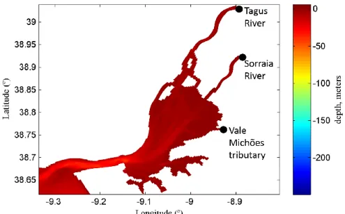
The Tagus estuary is one of the largest estuaries of the west coast of Europe and the largest of the Iberian Peninsula, having an East-West direction (Figure 2.1a), with a total area of 320 km2 (Valente and da Silva 2009) and with a mean volume of 1.8 km3_{(Freire and Andrade 1999). Its} mouth opens to a large bay in the adjacent coastal ocean, between Cape of Roca and Cape Espichel.

A deep, narrow inlet channel and a shallow inner bay compose the estuary. The inlet channel is 15 km long, 2 km wide and reaches depths of 40 m in some places (Figure 2.2), constituting the deepest part of the estuary (Fortunato et al, 1997). The inner bay is about 25 km long and 15 km wide, being the shallowest part of the estuary and has complex bottom topography with narrow channels, tidal flat areas and small islands on the inner most part of the estuary. Tidal flats corresponds to approximately 40% of the estuary’s total area, and are known to have an important role in Tagus estuary’s hydrodynamics by modifying the characteristics of the tidal wave (Fortunato et al. 1999; Fortunato and Oliveira 2005). The estuary is also characterized by the

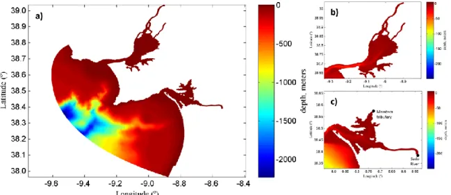
Figure 2.1: Study area: a) Geography of the Western Iberian System, showing the main features referred in the text. The 200 m bathymetric contour is shown, delimiting the continental shelf. From north to South: CO - Cape Ortegal; CF – Cape Finisterre; OC – Oporto Canyon; AC – Aveiro Canyon; CC – Cape Carvoeiro; CR – Cape Roca; CE – Cape Espichel; SB – Setubal Bay; CS – Cape Sines; CSV – Cape São Vicente; PC – Portimão Canyon; CSM – Cape Santa Maria. Adapted from Relvas et al. (2007); b) Bathymetries of Tagus and Sado estuaries and nearby coastal region.

(29)

existence of sand beaches, both in the inlet channel (northern margin) and in the inner bay (southern margin) (Freire and Andrade 2008).

The combined effects of low average depth, strong tidal currents, and high input river water make the Tagus a globally well-mixed estuary, with stratification being rare only in specific situations such as neap tides or after heavy rains. The Tagus estuary is meso-tidal and its circulation is mainly tidally driven. The amplitude of the tide is the controlling variable of the flow and is responsible largely for the turbidity of the Tagus, which in shallow areas of upstream part of the estuary is enhanced by small high frequency wind waves.

The tides are semi-diurnal, and the M2 harmonic constituent is dominant with amplitudes of 1 m (Fortunato et al., 1999), with tidal ranges varying from 0.75 m in neap tides in Cascais to 4.3 m in spring tides in upper estuary (Fortunato et al., 1997; Portela and Neves, 1994). The amplitudes of astronomic constituents grow rapidly in the lower estuary and more steady in the upper estuary and then decrease up to Vila Franca de Xira (Fortunato et al., 1999). The tidal amplitude is larger than offshore as a result of a small resonance effect (Oliveira, 1992). The surface velocities present typical values around 1 m s-1 _{and the salinity above 20 m depth is about 34 psu. At the bottom,} present salinity values of about 36 psu (typical oceanic values), except during high river runoff events, when lower salinity (around 34-35 psu) can be found(Vaz et al., 2009).

The influence of the river discharge seasonal variability is evidenced by several estimates for the water residence time within the Tagus estuary (Neves, 2010). As an example, Martins et al. (1983) reported a residence time between 6 and 65 days, respectively, for a river discharge between 2200 and 100 m3 _s-1_{, and 23 days for a mean river discharge of 350 m}3 _s-1_.

Figure 2.2: Location and bathymetry of Tagus estuary and the three freshwater inflows: Tagus river, Sorraia river and Vale Michões tributary.

(30)

In summary, the hydrography of the estuary is modulated by the tidal propagation and fluvial discharge from the major rivers, Tagus and Sorraia and Vale Michões tributaries.

2.2.1. Tributaries

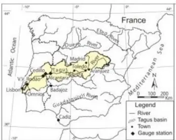
The Tagus River is the main source of freshwater of the estuary. The Tagus River is about 1038 km long, where 230 km are in Portugal, having a northeast-west direction as shown in Figure 2.1a. The river has a total catchment area of 80630 km2_{(Figure 2.3) (Vis et al., 2010).}

The discharge usually shows a pronounced dry/wet season signal and a large inter-annual variation (Valente and da Silva 2009). According to Macedo (2006), the Tagus River discharge regime has been modulated since the fifties, due to the building of the most important dams of the Tagus hydrographic basin. This author presented a study on the Tagus river discharge during the period between 1974 and 2001 at Almourol – about 130 km upstream of the estuary’s mouth - which showed a mean annual river discharge of 331 m3 _s-1_{and identified the year 1992 as a dry} year and 1979 as a wet year.

The river has an annual average discharge of 350 m3 _s-1_{, but varies greatly from summer to} winter between approximately 30 m3 _s-1_{in a dry summer and 2000 m}3 _s-1_{in a wet winter (Neves,} 2010), instantaneous records can reach flows of about 15000 m3 _s-1_{(Vaz et al., 2009).}

The river runoff can be calculated through the rainfall, this methodology is useful when the river discharge data is not available. Thus, a brief characterization of the rainfall is also presented. The mean annual rainfall in the Spanish Tagus basin for the 1949-2000 period was estimated at 655 mm (Egido et al., 2007), with a surface runoff of 11235 mm3_{. A mean rainfall for the total Tagus} basin for the period between 1940/1941 and 1992/1993 can be found in Appendix A (Serra, 2008).

(31)

The other two sources of freshwater of the Tagus estuary are the Sorraia River and the Vale Michões tributary.

The Sorraia River drainage system, an area measuring 7556 km2_{, is the largest basin inside the} Tagus River basin. The River forms at the confluence of Sor and Raia tributaries in Couço, flowing in a west direction towards the Tagus estuary. The Sorraia River has a length of 60 km from its source at Couço and a total length of 155 km from its longest source in Alentejo. The mean flow is about 39.5 m3 _s-1 _{(http://www.maretec.mohid.com/portugueseestuaries).}

The Vale Michões drainage system, an area measuring about 502 km2 _{is located in Tagus} River basin, flowing in a northwesterly direction from its source in Pegões until its confluence with Frio River, and flows directly in the Tagus estuary. The tributary has a total length of 36 km and it is characterized for the presence of four dams, used for irrigation and flood control. The flow of Vale Michões tributary is highly dependent of the rainfall.

2.3. Sado estuary

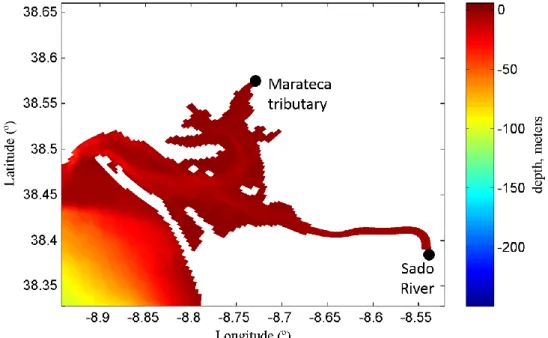
The Sado estuary is located 40 km south of Lisbon, Portugal, as shown in Figure 2.1b, with a South-West direction alignment in the Atlantic Ocean coast, with a total area of approximately 100 km2_{. It is about 20 km long and 4 km wide. The maximum depth is higher than 50 m and it has an} average depth of 8 m (Figure 2.4).

Several studies (Neves, 1982; Sobral, 1995; Wollast, 1979, 1978) highlighted the main processes controlling the circulation in the estuary and gave a first idea of its environment state.

Figure 2.4: Location and bathymetry of Sado estuary and the two freshwater flows: Sado River and Marateca tributary.

(32)

The flow is mainly tidally driven and very strong residual eddies exist inside the estuary associated with the curvature of the main channels. The lower estuary is occupied by two major eddies, while in the upper estuary the residual flow is more complex. This circulation supports the subdivision of the estuary in its upper and lower parts as suggested by Wollast (1979) based on temperature and salinity distributions.

The estuary has intertidal sandbanks that individualize a northern and a southern channel. The lower estuary behaves as a coastal lagoon with small freshwater influence, while the upper estuary has a freshwater dependent behavior (Martins et al., 2001).

The upper estuary has two main channels: the Alcácer channel on southeast and the Marateca channel on the north side, with 80% and 10% of total freshwater input to the estuary respectively, being the most important freshwater entrances to the estuary.

The tide is semidiurnal, with an amplitude of about 1.6 m in spring tides, and 0.6 m in neap tides. The most important harmonic constituents are M2 and S2. At the mouth, their amplitudes are 0.98 m and 0.35 m respectively, both being amplified inside the estuary. The low average depth, strong tidal currents and low freshwater discharge make the Sado a well-mixed estuary, which is stratified only rarely in specified situations such as high river discharges (Barton et al., 1998).

In summary, the tidal propagation and fluvial discharge from the Sado River and the Marateca Tributary modulate the hydrography of the estuary.

2.3.1. Tributaries

The Sado River drainage system, an area measuring 8341 km2_{, is bordered to the north by the} Tagus River basin and by the Guadiana and the Mira River basins to the south and east respectively. The Sado River basin excluding the estuary has a total catchment of 7692 km2 _{with a} mean altitude of 127 m (Figure 2.5a). The Sado River is approximately 180 km, initially flowing in a northwestward direction from its source in the Serra da Vigia (altitude of 230 m), then northward along the western coast of Portugal until its confluence with the Odivelas River, where it changes its course and flows in a more westward direction towards the Atlantic Ocean (Burke et al., 2011).

Following the same methodology for the calculation of the river runoff, through the rainfall, a brief characterization of the rainfall is also presented: the mean annual rainfall in the Sado River basin for the period between 1941/42 and 1990/91 was estimated is 621 mm, from which only 175 mm is surface runoff (with mean annual flow volume of 1350 hm3_).

The highest instantaneous peak flow was 2008 m3 _s-1_{in December of 1949 [Appendix B]. The} flow regime is very irregular being characterized by several months with very low flows or even without any flow (0.0 m3 _s-1_{in dry years) (Figure 2.5b).}

(33)

In summary, the Sado river flow displays a strong seasonal variability. In summer, monthly average values are lower than 1 m3 _s-1_{, while in winter the average values are about 60 m}3 _s-1_.

The other important freshwater source is the Marateca Tributary, located in Sado River basin (Figure 2.5a), flows directly into Sado estuary, having a total catchment of 134.07 km2_{and with a} length of 17.79 km. The flow is highly dependent of the rainfall, with observations from 2660 (1980/81) to 0.002 m3 _s-1 _{(1981/82) [Appendix B]}

2.4. Circulation patterns

The preferential north-south orientation of the continents that bound the Atlantic Ocean lead to meridional eastern and (intensified) western boundary currents which, together with the wind-induced zonal currents – westward flow under the trade winds, and eastward flow under the mid-latitude westerly winds, centred about a large sub-tropical atmospheric high-pressure cell – form the closed oceanic gyres. The ocean circulation system of the Iberian Basin is the result of different mechanisms of forcing and interactions with the open ocean circulation. An overview of some of these mechanisms, their importance and their consequences for the ocean circulation will be enounced.

The prevailing weather conditions in the Western Iberia Peninsula are conditioned by permanent factors, such as latitude, topography, influence of the Atlantic Ocean and the continental influence. The shoreline is also an important factor (Instituto de Meteorologia, 2004).

The western Iberia System is located in the northern limit of the Eastern North Atlantic Upwelling system (Peliz et al., 2002). The Iberian Peninsula is located in the Northern Hemisphere

Figure 2.5: Sado River: a) Basin location; b) Mean annual flow (mm). Adapted from http://www.peer.eu/about_peer/euraqua_collaboration/network_of_hydrological_observatories/.

(34)

Climatic Subtropical High-pressure Belt, in this particular case in the Azores Anticyclone (Peixoto and Oort 1992). The variability in the positioning of the Azores Anticyclone is closely related to the climatic variability of the West Iberia Peninsula.

The monthly regime of the winds is strongly dependent on the evolution of the atmospheric circulation on regional scales, being related with the latitudinal migration of the subtropical front and with the dynamics of the Azores Anticyclone cell (Fiúza et al., 1982). From March to August, the anticyclone centre moves along the 38°W meridian from 27°N to 33°N, respectively. From November to February it moves eastwards from 38°W and reaches 27°W in January, as a consequence of the relative increase of the winter high pressures located over Europe and Africa (Fiúza et al., 1982).

According to Instituto de Meteorologia (2004), the annual average values of pressure are between 1016 and 1020 hPa. The higher values (1030 hPa) and the lower values of pressure (980 hPa) occur in winter, leading to a higher pressure gradient, caused by the Azores Anticyclone development.

The near-surface circulation in the west coast of the Iberian Peninsula is primarily driven by the wind (Relvas et al., 2007), that repeats a seasonal cycle induced by the differences of atmospheric pressure already referenced in section 2.4.1. The winds that blow near the ocean surface change the vertical and horizontal density distribution (Vieira et al., 2000). This current system in the west coast of Iberia Peninsula is the Portugal Current system (PC), and reveals a strong seasonality and variability of mesoscale patterns.

The PC extends from about 36°N to 46°N and from the Iberian shores to about 24°W (Martins, 2002; Pérez et al., 2001). The PC itself is poorly defined spatially because of the complicated interactions between coastal and offshore currents, bottom topography, and water masses.

The system is comprised of the following main currents:

 The PC, which is a broad, slow, generally southward-flowing current that extends from about 10°W to about 24°W longitude;

 The Portugal Coastal Counter-Current (PCCC), a southward flowing surface current along the coast during winter season (Frouin et al., 1990; Peliz et al., 2005). This current transports to north warm and saltier water, from tropical regions, mainly over the narrow continental shelf to about 10-11°W longitude and flow from about 41-44°N

 The Portugal Coastal Current (PCC), a generally poleward current that dominates over the PCCC during the Summer and like the PCCC extends to about 10-11°W from

(35)

shore, also is present mainly from 41-44°N, where flow is 13.5 ± 5.7 cms-1_{(Martins, 2002;} Pérez et al., 2001).

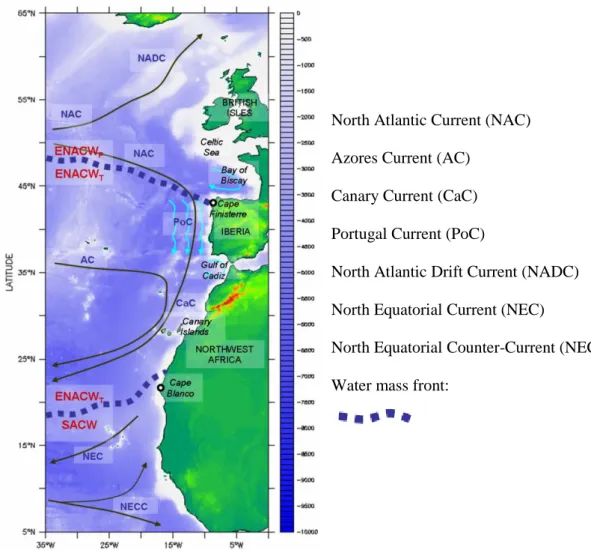
In Figure 2.6 are listed the main water masses and currents in the eastern North Atlantic region. The principal masses are Eastern North Atlantic Central Water of sub-polar (ENACWp) and sub-tropical (ENACWT) origins, and South Atlantic Central Water (SACW). The main large-scale surface currents are the North Atlantic Current (NAC), the Azores Current (AC), the Canary Current (CaC) and Portugal Current (PoC). Also shown are the North Atlantic Drift Current (NADC), the North Equatorial Current (NEC) and the North Equatorial Counter-Current (NECC).

The PC is supplied mainly by the intergyre zone in the North Atlantic, a region of weak circulation bounded to the north by the North Atlantic Current and to the south by the Azores Current (Pérez et al., 2001).

The PC System also suffers influence of seasonal winds, freshwater runoff from the Iberian

Figure 2.6: The eastern North Atlantic region. Principal currents in the eastern North Atlantic (Mason et al., 2010).

North Atlantic Current (NAC) Azores Current (AC)

Canary Current (CaC) Portugal Current (PoC)

North Atlantic Drift Current (NADC) North Equatorial Current (NEC)

North Equatorial Counter-Current (NECC) Water mass front:

(36)

Peninsula and the bottom topography (Ambar and Fiuza 1994; Pérez et al. 2001; Huthnance et al. 2002; Martins 2002). Meddies are also present, particularly in the region of the Tagus Abyssal Plain (about 11-13°W; 37-39°N) and along the shelf break, which are thought to be controlled mainly by the topography of the seafloor (Cherubin et al. 2000; Bower 2002; Coelho 2002; Huthnance et al. 2002).

According to Huthnance et al. (2002), the average flow of the top water column fluctuates according to season and varies more with increasing proximity to the shorecoast: northwards in autumn and winter, west and southwards in spring and summer (Martins, 2002; Pérez et al., 2001).

There are two major Rivers in the study area of west coast of Iberian Peninsula - Tagus and Sado. The river runoff is mainly dependent on rainfall (see section 2.2.1 and 2.3.1) and, therefore, is higher during winter. During this season, the slope and other shelf are under the influence of the Iberian Poleward Current (IPC) (Peliz et al., 2005). The IPC is a narrow (25-40 km) slope-trapped tongue – like structure that flows northerly along a distance exceeding 1500 km off the coasts of the Iberian Peninsula (DeCastro et al., 2011).

2.5. Summary of the characterization of the study area

In this chapter was presented a characterization of the topography, hydrography and dynamics of the Iberia Peninsula, with special attention to the Tagus and Sado estuaries and the nearby coastal region. This characterization allowed to identify and understand the role played by the major factors that establish the dynamics in this study area. A characterization of the hydrology of the rivers in terms of runoff was performed. The mean rainfall of the basins was also performed.

Thus, these factors will be taken into account in the next steps of this work, which aim the numerical model implementation.

(37)

Data presentation|19

3. Data presentation

The fate of a model simulation is largely determined by the inputs. These inputs reflect the accuracy on how to model certain physical processes. This section summarizes bathymetry, tide, wind and river discharge data used in the model.

3.1. Bathymetry

The bathymetry data used in the model was obtained from several sources. The coastal region bathymetry was constructed based on the General Bathymetric Chart of the Oceans (GEBCO). This bathymetric samples were given in format .xyz, the same format as Delft3D requires for bathymetry sample inputs, whereas the Tagus and Sado estuaries samples were obtained in Portuguese Hydrographic Institute (http://www.hidrografico.pt/) with shapefile format. The bathymetry of Tagus and Sado are a compilation of data surveys collected between 1964 and 2009, with spatial resolution of 100 m. Thus, it was necessary to use the software ArcGIS in order to convert the data to the format of .xyz.

3.2. Tidal forcing and initial conditions

Two different methods of tidal forcing are applied in the model implementation: one with the Portuguese Coast Operational Modelling System (PCOMS) (http://www.maretec.org/) and the other with TOPEX/POSEIDON data (MacMillan et al., 2004).

Transport conditions and tide propagation are calculated based on inputs from the Portuguese Coast Operational Modelling System (PCOMS) (http://www.maretec.org/). The tide propagation of PCOMS is given by FES2004 (Finite Element Solution). Two sets of data were collected, the year 2009-2010 and the year 2012. The system provides 3 days forecast of hourly ocean currents, sea surface height, water temperature and salinity. The year 2009-2010 (March 6 of 2009 to March 3 of 2010) comprise 50 vertical layers. The year 2012 (July 25 to December 31) comprise 47 vertical layers. The PCOMS domain has 0.06° (~6 km) of horizontal resolution.

The tide propagation for the second method are based in a global ocean tide model (NAO.99b model) representing the major 16 constituents with a spatial resolution of 0.25°, and have been estimated by assimilating about 5 years of TOPEX/POSEIDON altimeter data.

The propagation of the tide was interpolated across the open boundary using Matlab scripts, for a posterior implementation described in section 4.3.1.

(38)

20| Data presentation

3.3. Hydrographic

3.3.1. Water level

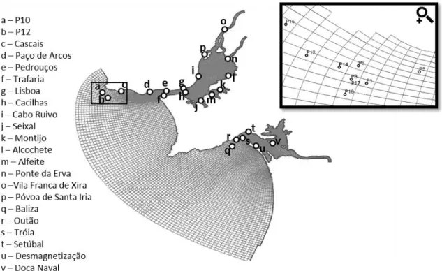
The data set available for this study are from three field surveys in Tagus estuary, one carried out in 1972, the second in 1981 and the third in 1986. The Sado estuary data are from six tidal stations placed along the estuary (Figure 3.1). Sea surface measurements presented in Table 3.1 were performed hourly during the period stated in the Time-series column, where Tagus data is given in water level value and Sado data in harmonics. This data set aims the calibration of the model.

In Figure 3.1 is also presented the location of stations referred in Table 3.1. The harmonic constituents used for Sado tide reconstruction were the M2, S2, N2, K2, K1, O1, P1, M4, MS4, L2, 2N2, NU2, MU2, T2, R2, Q1, 2Q1, RHO1, M3, S4 and 2SM2.

3.3.1. Salinity and water temperature

Water temperature and salinity offshore is described in several studies (Quintino et al., 2006; Santos et al., 2002; Silva et al., 2004) using a compilation of the available data surveys of 2009, on

Figure 3.1: Numerical grid and the location of the tide gauge, water temperature and salinity stations used in the model calibration (black square – grid zoom).

(39)

March 20, June 23, August 20 and October 15 and 16, obtained between 11 am and 4 pm, are summarised in Table 3.2.

Although more data were available for other stations, were not considered in this study due to the closest location between them, as shown in zoom area in Figure 3.1. The stations considered are shown in Figure 3.1. This data set aims the validation of the model.

Table 3.1: Sample Stations for water level.

Estuary Station Latitude (N) Longitude (W) Time-series

T agus Cascais 38°41’28.54’’ 9°25’02.35’’ 1986 Paço de Arcos 38°41’26.38’’ 9°17’37.29’’ 26-01-1972 31-12-1972 Pedrouços 38°41’36.40’’ 9°13’31.97’’ 28-09-1971 27-09-1972 Trafaria 38°40’32.07’’ 9°14’08.80’’ 1972 Cacilhas 38°41’59.64’’ 9°09’48.17’’ 1972 Lisboa 38°41’17.47’’ 9°08’53.25’’ 1972 Seixal 38°39’03.25’’ 9°04’38.73’’ 1972 Alfeite 38°40’05.34’’ 9°02’04.11’’ 09-04-1981 14-05-1981 Montijo 38°42’04.46’’ 8°58’36.36’’ 1972 Cabo Ruivo 38°45’56.26’’ 9°05’34.85’’ 1972 Alcochete 38°45’25.95’’ 8°57’57.84’’ 05-01-1972 31-12-1972 Ponta da Erva 38°49’35.68’’ 8°58’10.69’’ 1972

Póvoa de Santa Iria 38°51’23.39’’ 9°03’39.99’’ 04-08-1972 16-10-1972 Vila Franca de Xira 38°57’13.23’’ 8°59’09.59’’ 1972

Sad o Outão 38°29’32.80’’ 8°55’57.21’’ Harmonic constituents Baliza 38°27’02.59’’ 8°57’00.70’’ Tróia 38°29’37.53’’ 8°54’07.71’’ Setúbal 38°31’15.62’’ 8°53’05.39’’ Desmagnetização 38°28’00.19’’ 8°51’45.23’’ Setenave 38°28’18.94’’ 8°47’37.35’’

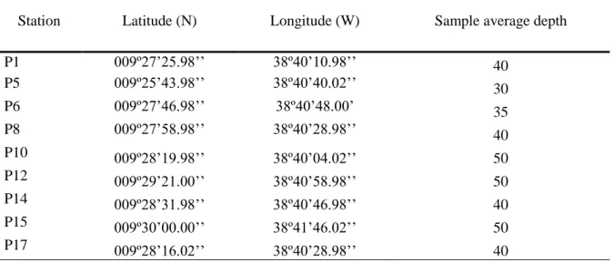
Table 3.2: Sample Stations for salinity and temperature.

Station Latitude (N) Longitude (W) Sample average depth

P1 009º27’25.98’’ 38º40’10.98’’ ₄₀ P5 009º25’43.98’’ 38º40’40.02’’ ₃₀ P6 009º27’46.98’’ 38º40’48.00’ ₃₅ P8 009º27’58.98’’ 38º40’28.98’’ ₄₀ P10 _{009º28’19.98’’} _{38º40’04.02’’} ₅₀ P12 _{009º29’21.00’’} _{38º40’58.98’’} ₅₀ P14 _{009º28’31.98’’} _{38º40’46.98’’} ₄₀ P15 _{009º30’00.00’’} _{38º41’46.02’’} ₅₀ P17 _{009º28’16.02’’} _{38º40’28.98’’} ₄₀

(40)

3.4. Meteorological

The atmospheric input used in this work was obtained from two different data sets, aiming the calibration of the model. The period obtained was June of 2009 to February of 2010 and July 27 to November 30 of 2012.

The air temperature, relative humidity and radiant heat flux was supplied by the National Center for Environmental Prediction (NCEP) model (http://www.ncep.noaa.gov/). The NCEP reanalysis (Kalnay et al., 1996) has a temporal resolution of 6 h. Several variables were obtained to calculate the radiant heat flux. This budget is composed of the net long and shortwave radiation flux across the atmosphere-ocean interface. Thus, the following variables were obtained: air temperature at 2 m; specific humidity; downwelling shortwave; upwelling shortwave and downwelling longwave.

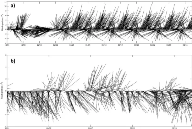
The wind and atmospheric pressure was supplied by Weather Research and Forecasting Model (WRF) (http://www.wrf-model.org). The WRF model version 3.6 (Skamarock et al., 2008) was applied for the study area. The application developed by Núcleo de Modelação Estuarina e Costeira (NMEC) comprises three two-way nested domains, where the parent domain has a horizontal resolution of 36 km, and the other two domains present 12 and 4 km of resolution, with a temporal resolution of 1 h. The vertical discretization was composed by 28 unequal spaced layers for each domain. The 4 km resolution domain was used between 37.414°N and 40.613°N and -12.709°W and -12.880°W, to generate the input for zonal and meridional wind at 10 m and the atmospheric

(41)

pressure. Figure 3.2a and 3.2b show the wind for the period of 2009/2010 and 2012, respectively. The wind direction tends to be northward for the period of 2009 – prescribing the winter pattern in this region, and southward for the period of 2012, characteristic of the summer season in the region.

3.5. River discharge

The daily river discharge data were obtained for the Tagus and Sado basin. The Portuguese Agency of Environment (http://www.apambiente.pt/), undertakes flow monitoring in a number of sites within Tagus and Sado River basin, with the longest series of records starting in the early 1930s, available in the internet at the Nacional System of Information of Hydric Resources (SNIRH) (http://snirh.apambiente.pt/).

According to APA there are 177 and 39 stream gauges stations in Tagus and Sado River Basin respectively, from which a significant number is presently inactive. Some stations have flow records, most of them during very short recording periods. From those stations, few are located in the Sorraia River and Vale Michões and Marateca tributaries, and most of them are presently deactivated. In this site it is also available other data, such as meteorological including rainfall.

After a brief analysis of the data available in SNIRH, it was observable numerous flaws, some days to months of data were missing for all the freshwater inflows and inexistence data for the Vale Michões and Marateca tributaries. Thus, a new search was needed to find time-series for the river discharges.

The Hydrological Predictions for the Environment (HYPE) (http://hypeweb.smhi.se/), from the Swedish Meteorological and Hydrological Institute (SMHI) has calculations of long-term series of several variables for the different basins in Europe, such as river discharges and rainfall. Through the HYPE v 2.1 was obtained time series of 30 years (01-01-1980 to 31-12-2010) for Tagus, Sorraia, Sado Rivers and Marateca and Vale Michões tributaries.

For a better approximation of the real freshwater temperature, the temperature of freshwater inputs is the air temperature provided by NCEP, due to the lack of information related to water temperature in both HYPE model and SNIRH database.

The missing discharge data for 2012 led to a research for methods that allow the prediction of discharges. Several documented methods for empirical formulas (Shaw, 1983) and cinematic formulas (Castiglioni et al., 2010) are limited to the hydrographic basin area, or require other variables on which there are no available data. According to Romano et al (2013), all approaches need long time series of rainfall as well as outflow of the basin during the year, in order to be calibrated and validated. Moreover, any methodology has been specifically developed to the

(42)

synthetic reconstruction of discharge time series, which is usually performed coupling methodologies devoted to the reconstruction of missing daily rainfall time series to one of the input-output models cited above. Thus, the main goal is to generate synthetic time series of discharge consistent with the observed precipitation regimen in the Tagus and Sado basins for 2012.

For this objective, in section 2 was made a research of the rainfall on the different basins of the five rivers. The datasets were obtained from the European Reanalysis and Observations for Monitoring, with a special resolution of 5 km and daily values of precipitation. Through the functional analysis, it was made a deconvolution of the discharge and precipitation time series for the 30 years (01-01-1980 to 31-12-2010), for all the five freshwater inputs, in order to filter the discharge time-series from the influence of the precipitation. Then, a convolution of the obtained signal was made with the precipitation time-series for the year 2012.

3.6. Summary of the inputs

This chapter presented the necessary inputs for the aims of this work: the bathymetry applied on the grid; the tidal forcing at the open boundaries; the hydrographic data such as water level, water temperature and salinity time series needful for the calibration and validation of the model; the atmospheric input used in the calibration and validation of the model, and in the spinups for the scenarios; and the river discharge used in this work.

Although several problems were encountered when acquiring the necessary data for the atmospheric and river discharge input, it was possible to set the necessary model runs to calibrate and validate the model, and to execute several scenarios.

Thus, these inputs will be taken into account in the next steps which aim the model calibration and validation, and further implementation of several scenarios.