Determinants of the Ex-dividend
day anomaly
The case of the London Stock Exchange
Eduardo Miguel Santos
Católica Porto Business School 2017
Determinants of the Ex-dividend
day anomaly
The case of the London Stock Exchange
Trabalho Final na modalidade de Dissertação apresentado à Universidade Católica Portuguesa
para obtenção do grau de mestre em Finanças
por
Eduardo Miguel Santos
sob orientação de
(PhD) Paulo Alexandre Pimenta Alves
Católica Porto Business School 2017
Acknowledgements
I would like to express my gratitude towards everyone who supported me throughout this research.
To my thesis advisor, Professor Paulo Alves, for all the guidance, availability and knowledge lent during this process.
To my parents, Artur and Fernanda, that always provided me with everything I needed and made me who I am today.
To my grandmother, Manuela, for her unconditional love.
To my girlfriend, Sofia, for always being there for me no matter what.
Abstract
This paper aims to investigate which are the determinants of the ex-dividend day anomaly, should it exist, and how they affect its outcome.
To study the characteristics of these determinants, a sample from the UK market was chosen for the period of 2007-2016. To explain the impact produced by these explanatory factors on ex-dividend day behaviour, a regression model was tested based on a similar methodology used by Barclay (1987), Boyd and Jagannathan (1994), Bell and Jenkinson (2002), amongst others.
The regression model suggests that, market capitalization, total assets growth rate and closely held shares are determinants of the ex-dividend day anomaly, having a positive relation with price-drop-to-dividend ratio. On the other hand price volatility and liquidity have a negative relationship with PDDR, being also significant explanatory factors of the ex-dividend day anomaly.
Abbreviation List
CE: Common equityCS: Closely held shares
CSO: Common shares outstanding DPR: Dividend payout ratio
MC: Market capitalization MTB: Market-to-book ratio NSGR: Net sales growth rate
PDDR: Price-drop-to-dividend-ratio PV: Price volatility
RE: Retained Earnings ROA: Return on assets TA: Total assets
TAGR: Total assets growth rate VO: Trading volume
Table of contents
Acknowledgements ... v
Abstract ... vii
Abbreviation List ... ix
List of Tables ... xiii
1. Introduction... 15
2. Literature Review ... 19
2.1. Ex-Dividend Day Anomaly ... 19
2.2. Dividend Policy Decision ... 22
3. Framework ... 34
4. Data and Preliminary Analysis ... 36
4.1 Sample Description ... 36
4.2. Preliminary Analysis ... 39
4.2.1. Spearman Correlation ... 39
4.2.2. Logarithmic transformation ... 39
4.2.3. Variable behaviour analysis ... 40
5. Methodology ... 45 6. Empirical Results ... 49 6.1. Regression ... 49 6.2. Discussion ... 51 7. Conclusion ... 56 Bibliography... 58
List of Tables
Table 1- Variable Description ... 37
Table 2 - Sample Descriptive Statistics ... 38
Table 3 - Relation of Explanatory Variables with PDDR ... 44
1. Introduction
The importance of dividends in the economical world is unquestionable, being utilized for different purposes. They can be used as a mechanism to mitigate agency cost, remunerate investors or simply signal a company’s future prospects. However dividends are one of the most intriguing things, especially when we relate them to ex-dividend price fluctuation. Dividend distribution causes stock price fluctuation between cum and ex-dividend day, but not always by the exact dividend amount.
The cum-dividend day is the last day a stock is tradable having its owner the right to receive the dividend amount. The ex-dividend-day, one day after the cum-dividend day, signalizes the first moment a stock trades after its dividend has been distributed.
Campbell and Beranek (1955) are the first two authors to observe the existence of an anomaly at the ex-dividend day. The authors state that the fall on the ex-dividend price at the ex-day isn’t equal to the amount of the distributed dividend. Contrarily, Miller and Modigliani (1961), assuming perfect market conditions, rational behaviour and perfect certainty, affirm that the fall on the ex-dividend price should be exactly the same as the dividend value.
Elton and Gruber (1970), Heath and Jarrow (1988) Boyd and Jagannathan (1994), and many others, prove by different theorems that the anomaly observed at the ex-dividend day exists, stating that the ex-dividend price fall is different than the dividend amount.
However, before dividends reach the pockets of investors, company managers have to decide whether or not to distribute them. In other words,
insiders have to decide, based on several factors, the company’s dividend distribution policy.
John Lintner (1956), elaborates a model which studies the behaviour of corporate dividend policy. The author points out the importance of building a target payout ratio, and that investment opportunities and retained earnings, play a major role on managers’ payout decision, regarding the timing and the amount of the distributed dividend.
Once again, Miller and Modigliani (1961), assuming specific market conditions, create a model in which they prove that dividend distribution policy has no impact on share price.
Several years’ later authors such as Rozeff (1982) and La Porta et al (2000) focus their research on the way transaction costs and agency costs contribute to dividend payout ratio.
Fama and French (2001), DeAngelo, H., DeAngelo, L. and Stulz (2004) investigate the likelihood of firm paying dividends, always controlling for firm characteristics, concluding that factors like size, profitability, growth perspective amongst other, have an impact on the probability of firms paying dividends.
The main reason for the execution of the present study focuses on the possibility to contribute to the financial literature, connecting two important matters: dividend policy and ex-dividend price behaviour. Hence the principal goal of this research relies on comprehending which are the ex-dividend anomaly determinants, based on the firm characteristics that influence managers’ decisions concerning dividend policy.
In order to test for the determinants of the ex-dividend day anomaly, a single well known methodology was applied, assuming however different explanatory variables.
Using an OLS regression model, several firm characteristics and other explanatory variables were regressed against the price-drop-to-dividend ratio. Analysing the outcome of the model we can conclude that price volatility, closely held shares, market capitalization, total assets growth rate and liquidity, are determinants of the PDDR.
The current dissertation has the following structure: Section 2 considers valuable literature regarding ex-day anomaly explanation and dividend policy decision; Section 3 describes and justifies the merge of both perspectives; Section 4 characterizes the sample data and gives an initial analysis; Section 5 presents the chosen methodology; Empirical results are discussed and presented at Section 6; Section 7 closes the current study with the main conclusions.
2. Literature Review
2.1. Ex-Dividend Day Anomaly
Campbell and Beranek (1955) were the first to question that a stock price should drop by approximately the amount of the dividend at the ex-dividend date. Let it be known that the ex-dividend date, represents the first day that a stock trades without dividend, and where the owner of the security will receive the amount of the expected dividend. The cum-dividend date is the last day a stock trades with owner/buyer of this stock, having the right to receive it.
They reached the conclusion that, the average stock price drop-off on the ex-dividend date was 90% of the ex-dividend amount.
Finally, the authors state that a tax-paying individual will have advantage in selling before the ex-dividend date, but in the case of buying, only after it. Although they could not find any evidence on why the stock behaved in this way, they were the first to question and point out that an anomaly existed.
Some years later came the first hypothesis that would try to explain this behavior on the ex-dividend date. Elton and Gruber (1970) explored the way in which tax rates would affect this stock price drop-off on the ex-dividend day. They start by stating that a stock, which is sold at the ex-dividend day, will allow the seller to receive the dividend previously, but will make him sell the stock at a much lower price than he would, if he sold it before it went ex-dividend. They also explain that in a rational market, the fall in price that results from the ex-dividend date, must show the dividends value.
The tax-effect, as called by the authors, consists on analyzing the differences between capital gains and dividends taxation. If the tax rate applied to capital gains is lower than the tax rate applied to dividends, then, for example, a dollar of capital gains is worth more than a dollar of dividends.
They claimed that when investors were thinking of selling a stock near to its ex-dividend date, they would calculate whether they were better off selling just before it goes ex-dividend, at the cum-dividend date, or just after. However, they state that, at equilibrium, the marginal investor should consider to be indifferent selling at either the ex-dividend date, or the cum-dividend date. The equation that translates this equilibrium, assuming risk neutral investors and no transaction costs, is given by:
, (1)
Where is the stock closing price at the cum-dividend day, is the stock closing price at the ex-dividend day, is the stock price at the time it is bought, represents the dividend value, is the tax rate for dividends and is the tax rate for capital gains.
However, if equation (1) is re-arranged, we have:
(2)
is a mathematical expression that was known as price-drop-to-dividend ratio, or PDDR.
However, if we use the ex-dividend rate return instead of PDDR we obtain:
(3)
the PDDR and the dividend yield are positively correlated. Hence, the bigger the dividend yield, the bigger the PDDR, and the closer the fall of the stock’s price is to the dividend’s value. The other explanatory variable included in the model, was the firm’s payout ratio. The evidence was in line with Modigliani’s and Miller’s clientele effect, suggesting that a variation in the company dividend policy will have consequences on shareholders wealth.
The clientele effect hypothesis consists on investors with high marginal tax rate preferring a high dividend yield.
However, other authors disagree with this explanation and present different hypothesis to explain this anomaly.
Kalay (1982) presents the short term-trading hypothesis. This author states that the transaction costs implicit in the dividend capturing strategy at the short-term, have an impact at the stock price variation on the ex-dividend day. On the other hand, Heath and Jarrow (1988), prove by a theorem, that in an economy without transaction costs (frictionless economy), there are no arbitrage opportunities, even though the change in the dividend stock price at the ex-dividend day, can be different from the ex-dividend value. They demonstrate that a short-term trader can’t build such an arbitrage position, unless he knows before the ex-dividend date (with 100% probability), if he should buy the stock and capture the dividend or short sell the stock and sell the dividend. It is impossible for the trader to know this, before the ex-dividend instant, unless he knows that the stock price drop is always above or below the dividend.
Eades, Hess and Kim (1984) study the relation of the ex-dividend day stocks that have a high dividend yield. It is pointed out by the authors that dividend-capturing strategies can be the main reason to influence the behavior of the stock price, at ex-dividend date price. Lakonishok and Vermaelen (1986) confirm this view and add that the number of transactions made between the
cum-date and ex-date (the abnormal trading volume) is associated with the dividend yield.
Boyd and Jagannathan (1994), reinforce the importance of the presence of transaction costs in the study of the pricing at the ex-dividend day. Moreover, both authors support the idea that we should not focus our research in assuming that all investors have a taxation preference for capital gains instead of dividends. Boyd and Jagannathan (1994) create a model that analyzes the relation between the dividend yield and the expected amount of the price drop at the ex-dividend date. The model includes three types of traders and gives a special emphasis to transaction costs. The authors conclude that there exists a nonlinear relation between a stock’s dividend yield and the percentage of the price drop, at the ex-date.
2.2. Dividend Policy Decision
Lintner (1956) studied the behavior of corporate dividend policy through a detailed field investigation, interviewing two to five high-ranked positions at the selected companies. Lintner (1956) centered his study on over 600 listed firms (where 28 were chosen for a more detail research), using fifteen traits that are related or are expected to be related to the decision of dividend policies and payments, hence building a theoretical model of corporate dividend behavior. In his model, a regression is created, including: the variation of dividends between the present year ( ) and the year before ( -1); the amount of dividends of the preceding year and the profits after taxes for the present year.
Throughout the investigation, the author characterizes the manager’s behavior as conservative, stating that the main issue is not in the dimension of the change of the dividend rate, but rather if it changes or not. This aversion to change and delay (speed of adjustment) concerning the dividend rate, forms a
be justified in a logical, safe, resounding way, for internal and external stakeholders. However, the author states that although dividend rate my go up with the rise of earnings, payout ratio tends to drop. Current net earnings were the best financial indicator to use in order to justify changes. Not only for their periodical updates through reporting documents, but also because stockholders had direct interest in them. Hence, Lintner (1956) concludes that big fluctuations in earnings, or at the level of earnings, were one of the most important determinants to dividend policy.
He also emphasizes the relevance of the dividend payout ratio. Companies would act based on the target payout ratio they had set up. Industry growth perspectives, management view on stockholders preferences, favorable access to capital markets, among others, help to build the perfect target payout ratio thanks to their predictive capacity. Creating an ideal payout ratio, which can predict future profits, is considered by the author to be one of the most powerful influences of dividend policy. Lintner (1956), also highlights the importance of current investment opportunities. Through his model, he claims that the amount of money directed towards investments has a high correlation with profits, volume of sales and company funds. The relationship between these variables is taken in count when corporate dividend policy is elaborated, allowing firms to create consistency in payments over long periods.
Modigliani and Miller (1961), produce a very well-known theory that defends the irrelevance of dividend policy, on stock’s price fluctuations at specific market conditions. The authors study this behavior assuming: perfect market conditions (where no investor’s action has impact on price formation, asymmetric information doesn’t exist, no tax cost nor transaction cost whether stock’s are bought, sold or issued, no tax differences between capital gains and dividends), rational behavior (investors only care about increases on their own
dividend increase), perfect certainty (where investors are fully sure about a firm’s investing program and future profits).
Modigliani and Miller (1961, p. 412) conclude, amongst other things, that “(…) the price of each share must be such that the rate of return (dividends plus capital gains per dollar invested) on every share will be the same throughout the market over any given interval of time.” They use this statement as a starting point, to further prove, analytically, the irrelevance of dividend policy on share price determination. The following equation demonstrates what the authors consider to be the composition of the share price:
independent of ; (3)
or equivalently,
(4)
Where = dividends per share paid by firm during period , = the price (ex any dividend in - 1) of a share in firm at the start of period (Modigliani and Miller, 1961, p. 412). In order to analyze the impact of dividend policy, the authors decide to restate equation (4) in terms of the total firm value:
= . (5)
Where = the number of shares of record at the start of , = the number of new shares (if any) sold during t at the ex dividend closing price so that, = + , = = the total value of the enterprise and = = the total dividends paid during to holders of record at the start of (Modigliani and Miller, 1961, p. 413).
The authors then present three possible ways that dividends can affect the firm’s share price. In order to make it easier to understand the three terms the authors suggest, we shall rearrange equation (5)
(6)
Modigliani and Miller (1961) recognize that current dividends have a direct influence on the firms total value (and equivalently, on the firm’s shares)
through the first term of the equation ( ). On the second term ( dividends have, supposedly, a indirect effect on the share’s price. However, this could only happen if was a function of future dividend policy and had information related to future dividend policy. Nevertheless, the investigators have very solid assumptions, stating that future dividend policy is known (as all the rest of the periods), being independent of the current dividend distribution choice. Therefore, , will be independent of the
actual dividend decision. Dividends have through the third term ( ), a
indirect effect on the company’s total value, related to the new shares sold to outside investors during . According to Modigliani and Miller (1961), these two ways affect in a contradictory form, ending up canceling out each other. By expressing in terms of , the authors demonstrate that does not constitute the equation’s arguments, directly. “Specifically, if is the given level of the firm's investment or increase in its holding of physical assets in t and if is the firm's total net profit for the period, we know that the amount of outside capital required will be:
Afterwards, if we substitute expression (7) into (6), we obtain:
(8)
Consequently, these authors conclude that the dividend payout policy used in , won’t affect the share price at .
Fama and Babiak (1968) work on top of Lintners’ (1956) model, making a few changes to it. The authors’ suppress the constant term from the regression, and add the amount of earnings for the previous year -1. They perform various statistical tests with different models, adding the lagged earnings and suppressing the constant variable, changing the sample and examining the estimation of the coefficients. After testing various alternative models, Fama and Babiak (1968) conclude that the model based on Lintner (1956), with the addition of the lagged earnings and the suppression of the constant term, is the one with more explanatory power.
Rozeff (1982), focuses his research on a different, yet related, subject. The dividend payout ratio. From 1974 to 1980 he calculates the average of seven payout ratios, over seven years, chosen from a pilot test for 200 firms. The author analyzes the patterns over these years concluding that such period was the most indicated one, as it smoothed the cases of earnings fluctuations and did not produce measurement errors related to constant variations the ratio’s mean value. His approach concerns the search for an optimal dividend payout ratio, and, which are the determinants of this variable. In order to examine what influences the dependent variable, Rozeff (1982) introduces the importance of transaction costs associated to the issuance of external financing, as well as agency costs related to the same matter. According to the author, dividends are used as a regulator between shareholders and managers interests, allowing the
investment are. This happens because normally, dividend distribution happens at the same time that the company is increasing its capital externally, to support current and future investment. Therefore, stockholders are aware that the firm is financing the dividend thanks to external funds, which have a cost. Although this can be costly, stockholders receive new information associated to management prospections, hence minimizing agency costs.
Rozeff (1982) uses three variables to form transaction costs: realized growth rate (from 1974-1979), forecast of the growth (1979-1984), and the beta coefficient. The author justifies the choice of the first two variables stating that if past growth were fast, ceteris paribus, the firm would hold the funds to avoid external financing which has a cost. The same thing holds for future growth perspectives, making the manager establish a lower payout ratio. As for the beta coefficient, the author hypothesis that a high operating and financial leverage, leaving all the rest constant, will lead to the choice of a lower dividend payout ratio, so that the firm is protected from external costs. The beta coefficient, as is popularly known in the financial theory thanks to the hamada model (Hamada, 1971), is a proxy for operating and financial leverage.
In order to build the agency costs variable, Rozeff (1982) uses: percentage of stock held by insiders and the number of common stockholders. According to the author, summing two opposing costs, will determine the optimal dividend payout.
Having as sample 1000 companies, Rozeff (1982) performs multiple regression tests. He corroborates the hypothesis considered in his research, concluding that higher growth rates, higher beta coefficients and higher inside ownership, lead to lower payout ratios. As for the stockholders, a great number of common stockholders is associated to a large dividend payout.
two models that relate agency costs, using shareholder protection as proxy, with higher or lower payout ratios, in a cross-section analyses that includes more than 4000 companies over 33 different countries. Shareholder protection is measured in the models by the use of 2 dummy variables. The first equals to one if: “(…) a country’s company law or commercial code is of civil origin, and zero for common law origin.” (La Porta et all, 2000, p.10). The second dummy is equals to one if: “(…) the index of antidirector rights is below the sample median.” (La Porta et all, 2000, p.10). Antidirector rights reflect voting rights, which allow minority shareholders to call an extraordinary shareholder meeting, vote for directors, amongst others.
The authors state that the way insiders control the companies’ operations determines the relationship between controlling shareholders and managers, and minority shareholders. If insiders wish to use their controlling power for personal benefit, making decisions that put at risk the firms’ future success by investing in non-value-maximizing opportunities, then the bond with minority shareholders will obviously degrade. Therefore, dividend distribution are a way to provide more internal information to outside investors, returning what was invested to outside stockholders, disabling insiders to use retained cash for personal benefits. Besides dividend distribution, the law can also give minority stockholders, through the right to receive the same dividend per share as inside stockholders, or the right to sue the firm for inappropriate actions, a legal mechanism of protection against insiders’ decisions.
The “outcome model”, as entitled by the authors, tests different shareholder quality protection in many countries, comparing it to the amount of dividend payout given by the company. The “outcome model” concludes that, ceteris paribus, countries with better shareholder protection have a higher dividend payout ratio. It also adds that companies, which have good investment
opportunities that are inside countries, which have good shareholder protection, should have a lower payout ratio.
The “substitute model”, as called by the authors, tests the role dividends take as substitutes for legal protection of stockholders. Companies that decide to pay dividends which belong to countries that have fragile legal protection, build good reputation for a fair stockholder treatment. In these cases, shareholders can’t rely on other mechanisms to guarantee an impartial treatment. Hence, this vision defends that, ceteris paribus, payout ratios should be higher in countries that have worse legal protection than in other countries which have a solid protection.
The “substitute” model concludes, as La Porta et al (2000) state that: “(…) in countries with poor shareholder protection, firms with better investment opportunities might pay out more to maintain reputations.” (p.8)
Fama and French (2001), study the number of dividend paying firms from 1926-99. Through this research, they conclude that dividend payers harshly decrease after 1978. In terms of percentages, the number of payers were at 66,5% in 1978, but by the time the year 1999 was reached, only 20,8% of companies payed dividends. Three questions are raised by the authors, which are answered by logit regressions and summary statistics to examine the characteristics of dividend paying firms. Fama and French (2001) address these three questions: “(…) (i) What are the characteristics of dividend payers? (ii) Is the decline in the percent of payers due to a decline in the prevalence of these characteristics among publicly traded firms, or (iii) have firms with the characteristics typical of dividend payers become less likely to pay?” (p. 4)
According to the authors, both methods (logit regressions and summary statistics) indicate that profitability, investment opportunities and size, influence dividend policy. Dividend payers have higher profitability (measured
terms of assets), and have less investment opportunities (measured as R&D expenditures) than non-dividend payers. Both profitability and size are associated to a higher capacity of distributing cash (in the form of dividends). Regarding investment opportunities, the higher they are, the higher are the funds that a company must retain for those investments (hence less cash is distributed in the form of dividends).
Fama and French (2001) point out that the decline on dividend payment after 1978 is partially influenced by the shift in firm characteristics. From paying dividend firms to the characteristics of firms that have never paid dividends – “(…) low earnings, strong investments, and small size.” (p.4). A big wave of firms with small profitability but with huge investments which never paid dividends, are responsible for the big downward shift in dividend payment. The other part, which influences the decrease on dividend payment, is related to the fact that firms are simply not paying so much dividends, regardless of their characteristics. The authors state that whatever the benefits that dividends bring, they simply have decreased year after year.
DeAngelo. H., DeAngelo, L. and Stulz (2004), examine the relation between retained earnings and the likelihood to pay dividends, controlling for several firm characteristics. To test the hypothesis of, the increase in the probability to pay dividends by the firm, with higher levels of retained earnings (earned equity), a variety of multivariate logit models are used. The analysis is restricted to nonfinancial and nonutility firms, between 1973-2002. The authors start by highlighting the importance of dividend distribution by companies. They investigate what no other study has, and conclude that “(…) had the 25 largest long-standing dividend-paying industrial firms in 2002 not paid dividends” (p.1), they would have $1.8 trillion of retained cash, missing innumerous investment opportunities. Besides, without any information being
have increasingly more reasons to adopt new policies for personal benefit. Hence, a continuous flow of dividend distribution will reduce the threat of agency conflicts.
DeAngelo. H., DeAngelo, L. and Stulz (2004), measure earned equity by firms in two distinct ways. Assuming that the main determinant of the choice to pay dividends is common equity, the authors calculate retained earnings (RE) over common equity (CE) (RE/CE). In the case of the main determinant of the decision to pay dividends relays on the amount of total assets, then RE over Total Assets (TA) is calculated (RE/TA). The authors also consider the examination of investment opportunities, proxied by market-to-book ratio, asset growth rate and sales growth rate, as they recognize that investment opportunities affect dividend distribution policy. The following explanatory variables are also included in the model: “(…) (iii) profitability, as measured by the current period return on assets (ROA), (iv) growth, as measured by the sales growth rate (SGR), asset growth rate (AGR), and market-to-book ratio (M/B)), (v) size, as measured by the asset (NYA) and equity value (NYE) percentiles for firms listed on the NYSE, and (vi) holdings of cash plus marketable securities as a fraction of total assets (Cash/TA).” (DeAngelo. H., DeAngelo, L. & Stulz, 2004, p.8-9).
The three researchers conclude that dividend-paying firms usually have higher amounts of earned equity than non-paying dividend firms. Moreover, the results show that dividend-paying companies are larger and more profitable than non-paying dividend firms (consistent with Fama and French, 2001, results). Once again, the probability of a firm paying dividends has a positive relation with size and profitability, and a negative one with growth. Relating to the main hypotheses to be tested, the authors select the dependent variable as the payment/nonpayment of dividends in a certain year, and RE/TE
or RE/TA as explanatory variables, adding also several control variables, to create several logit regressions.
After adding RE/TE to the control variables (the basic model used by Fama and French), the authors concluded that RE/TE and the probability to pay dividends are highly correlated.
When DeAngelo. H., DeAngelo, L. and Stulz (2004) substitute RE/TE for RE/TA, using now total assets as denominator (that according to the authors may include puzzling features of debt policy, and that’s why RE/TE is preferred over RE/TA), the results are the same. RE/TA maintains a strong relation between the probability of a firm paying dividends and the amount of earned equity it detains.
Denis and Osobov (2008), analyze the tendency to distribute dividends on developed financial markets (United States of America, the United Kingdom, France, Germany, Canada and Japan) from 1982-2002. Additionally, the authors examine the similarity of characteristics of paying and non-paying firms (across all countries) and the possible mutation these characteristics may have suffered throughout the times.
Denis and Osobov (2008) results corroborate Fama and French (2001) analysis, showing once again that the probability of a firm paying dividends is related to its size, profitability and growth opportunities. Similarly to DeAngelo, H., DeAngelo, L. and Stulz (2004) research, Denis and Osobov (2008) conclude that the possibility of paying dividends is powerfully related to the ratio of retained earnings to total equity. Additionally, in all countries that constitute the sample, bigger, more profitable, and with a bigger amount of earned equity, have a higher likelihood of paying dividends. Related to the quantity of dividend payers, also studied by Fama and French (2001) for USA firms, the authors conclude that the declining tendency also happens on the
This investigation aims to provide better insights on which are the determinants that explain the anomaly, occurring at the ex-dividend-date, namely the PDDR. Moreover, it intends to explain whether or not, firm characteristics, amongst other explanatory variables, have a direct impact on the price-drop-to-dividend ratio.
3. Framework
The available literature considering dividend issues is vast. From dividend policy to ex-dividend anomalies, many questions are investigated, answered and defended, whilst other queries remain unsolved.
After analysing which are the variables that affect dividend distribution decision, alongside with which are the explanatory factors that influence the ex-dividend price behaviour, a regression model was created. The principal motivation for this research relies on the contribution these elements have on the explanation of the PDDR. The rationale behind the chosen variables for this model is simple. Managers and highly-ranked insiders have in consideration various factors which help them decide whether or not to distribute dividends. As proven by several empirical investigations (Lintner 1956, Rozeff 1982, La Porta et al 2000, Fama and French 2001, DeAngelo, H., DeAngelo, L. & Stulz 2004) these variables have a direct impact on the decision to distribute dividends and the likelihood to pay them. If dividend policy is so highly influenced by these variables, it is logical to ponder that the observed anomaly at the ex-dividend day can also be explained by the impact of these variables, directly. On the other hand, researchers such as Campbell and Beranek (1955), Elton and Gruber (1970), Kalay (1982), Eades, Hess and Kim (1984), Lakonishok and Vermaelen (1986), Boyd and Jagannathan (1994), present us different theories related to the preferences of a marginal investor and how specific market and trading characteristics, contribute to the explanation of the anomaly.
We then have two distinct matters from which we can infer many conclusions regarding dividends. On one side we have managerial decisions
operational/financial characteristics and agency costs regulating mechanisms. A dividend policy decision view, based on company performance and evolution. On the other we have marginal investors’ actions, regarding market transactions and dividend return rates, and the way they influence PDDR. An explanation of the ex-dividend day anomaly, based on marginal investors’ activities. After aligning these two visions and selecting the best explanatory features of both, a regression model was created with the purpose of explaining the PDDR fluctuation. Sample data will be presented at section 4. The following model will be explained in more detail at section 5.
In order to maximize the quality of obtained information, a market with big company diversity, impact at a worldwide level, and high transaction dynamic was required. The UK market hosts a large diversity of companies, ranging from big to small scaled, from numerous sectors. This diversity allows for a larger variety of dividend policy decisions, higher likelihood of ex-dividend day anomaly cases, and a wider range of investors’ actions which have an impact on the market. The bigger the probability of accommodating different managerial and investing perspectives, the more explanatory power it confers to the research.
The UK market however, has a particular trait. It is important to notice that UK companies distribute dividends more than once a year. It is common to find firms which distribute dividends twice or even four times a year (semester or trimester basis). For the existing investigation, we will use the latest dividend values presented by each company.
4. Data and Preliminary Analysis
4.1 Sample Description
The sample data used to investigate the predictable power of certain variables in respect to the PDDR, was taken from the firms that constitute London Stock Exchange. The chosen period for analysis ranges from the 1st of January of 2007 to the 31st of December of 2016, including companies that were active at least for 1 year between the selected period. For this set of firms, data was collected respecting the company’s market capitalization, return on assets, total assets, turnover by volume, retained earnings, price volatility, total assets annual growth rate, net sales annual growth rate, ex-dividend date and the respective closing adjusted price, cum-dividend date and respective adjusted price, dividend rate date and respective adjusted price, common shares outstanding, closely held shares, dividend yield and the dividend payout ratio. All data was extracted from Thomson Reuters Datastream database.
In order to conduct the regression that will attempt to explain the anomaly at the ex-dividend day, several preliminary measures were followed. These procedures will be presented in more detail in the following section. After these testes were made, the following variables which compose the model are defined at Table 1.
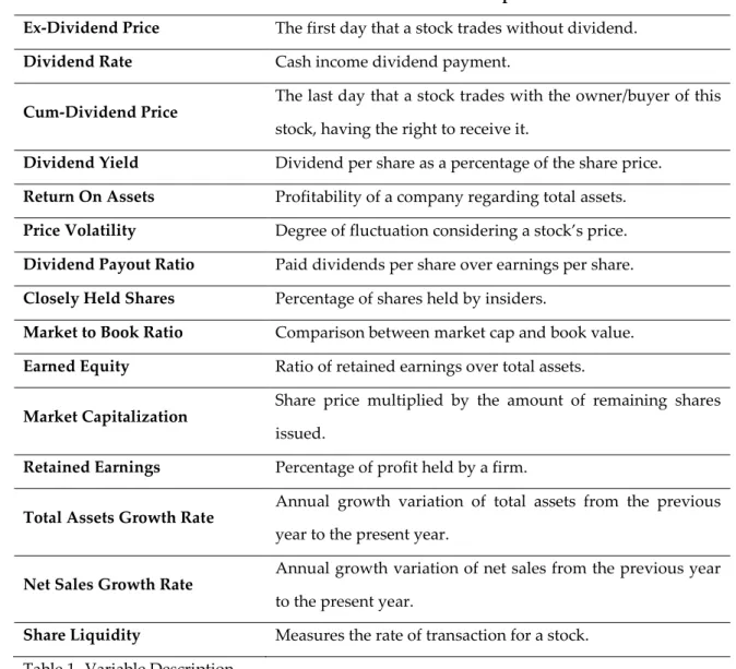
Variables Description
Ex-Dividend Price The first day that a stock trades without dividend.
Dividend Rate Cash income dividend payment.
Cum-Dividend Price The last day that a stock trades with the owner/buyer of this
stock, having the right to receive it.
Dividend Yield Dividend per share as a percentage of the share price.
Return On Assets Profitability of a company regarding total assets.
Price Volatility Degree of fluctuation considering a stock’s price.
Dividend Payout Ratio Paid dividends per share over earnings per share.
Closely Held Shares Percentage of shares held by insiders.
Market to Book Ratio Comparison between market cap and book value.
Earned Equity Ratio of retained earnings over total assets.
Market Capitalization Share price multiplied by the amount of remaining shares
issued.
Retained Earnings Percentage of profit held by a firm.
Total Assets Growth Rate Annual growth variation of total assets from the previous
year to the present year.
Net Sales Growth Rate Annual growth variation of net sales from the previous year
to the present year.
Share Liquidity Measures the rate of transaction for a stock.
Table 1- Variable Description
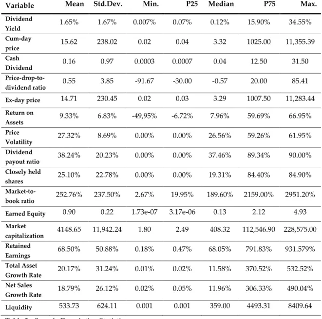
Table 2 presents the summary statistics for the variables that constitute the model. Sample data referring to the UK market has a total of 2767 observations.
Variable Mean Std.Dev. Min. P25 Median P75 Max. Dividend Yield 1.65% 1.67% 0.007% 0.07% 0.12% 15.90% 34.55% Cum-day price 15.62 238.02 0.02 0.04 3.32 1025.00 11,355.39 Cash Dividend 0.16 0.97 0.0003 0.0007 0.04 12.50 31.50 Price-drop-to-dividend ratio 0.55 3.85 -91.67 -30.00 -0.57 20.00 85.41 Ex-day price 14.71 230.45 0.02 0.03 3.29 1007.50 11,283.44 Return on Assets 9.33% 6.83% -49,95% -6.72% 7.96% 59.69% 66.95% Price Volatility 27.32% 8.69% 0.00% 0.00% 26.56% 59.26% 61.95% Dividend payout ratio 38.24% 20.23% 0.00% 0.00% 37.46% 89.34% 90.00% Closely held shares 25.10% 22.78% 0.00% 0.00% 19.31% 84.40% 84.90% Market-to-book ratio 252.76% 237.50% 2.67% 19.95% 189.60% 2159.00% 2951.20%
Earned Equity 0.90 0.22 1.73e-07 3.17e-06 0.13 2.12 4.93
Market capitalization 4148.65 11,942.24 1.80 2.49 408.32 112,546.90 228,575.00 Retained Earnings 68.50% 50.88% 0.18% 0.47% 68.05% 791.83% 931.579% Total Asset Growth Rate 20.17% 31.24% 0.01% 0.02% 11.58% 370.52% 532.52% Net Sales Growth Rate 18.79% 26.12% 0.02% 0.05% 11.96% 306.33% 490.04% Liquidity 533.73 624.11 0.001 0.001 359.00 4493.31 8409.64
4.2. Preliminary Analysis
4.2.1. Spearman Correlation
Multicollinearity is a common problem amongst explanatory variables in a regression model. It occurs when the predictors are perfectly collinear with each other, indicating that we will not be able to distinct the effects of the different variables. Even though coefficients can be calculated, variables which have a close linear combination of each other can cause estimation problems. For example, although multicollinearity does not decrease the explanatory power of the model as a whole, it influences the individual calculation of each explanatory variable. In order to correct for this issue, we should drop one or more variables that cause the problem.
Due to non-normality issues related to some predictors, Spearman correlation will be used to evaluate the degree of correlation between all the paired explanatory variables. Coefficient interpretation is very similar to Pearson’s. The closer the correlation between variables is to 1, the stronger the monotonic relationship. Assuming that any correlation above 0.8 or below -0.8 may induce multicollinearity complications, due to the strong correlation between paired variables, some predictors who meet this value will be dropped.
After completing the correlation tests’, total assets, trading volume, common shares outstanding and common equity won’t be included in the model, as they don’t follow the required conditions.
4.2.2. Logarithmic transformation
Skewness is a statistical measure that characterizes the asymmetry from the normal distribution of a variable on a sample set. Several cases of positive high
may derive from excess of skewness, a logarithmic transformation was completed for the following variables: total assets, common shares outstanding, common equity, trading volume. Logarithmic transformation allows for skewness correction (bringing it much closer to a 0 value), and hence normalizing the distribution of its variable.
4.2.3. Variable behaviour analysis
Some variables that compose the regression model that will be analyzed at section 6, have never been used to explain the PDDR. However, other investigators have used them in order to examine other queries related to the dividend issue. We can then try and predict the behavior of these explanatory variables based on some economic rationale. Let us note that this predictability exercise is merely hypothetical.
DeAngelo, H., DeAngelo, L. and Stulz (2004) study the relationship between retained earnings and the probability to pay dividends, controlling for several firm features. Return on Assets (ROA), is used by the authors to measure the profitability of a company. They conclude that the probability of a firm paying dividends has a positive relation with profitability. Therefore, it has a positive impact on the managerial decision to distribute dividends. The assets of a company can be on both sides of the balance sheet (debt and equity), and in order to fund the operational activity of a firm, both debt and equity can be used. Investors will then want to analyze the ROA indicator as it will help explain how well a firm is handling their assets. We can state that, on average, the higher the ROA, the better the capacity that a company has to transform investment into profit. Hence we expect that ROA has a positive relation with the PDDR.
Price volatility measures a stock average annual price movement, considering high and low variation from its mean price for each year. For example, a stock's price volatility of 10% shows that the stock's annual high and low price has a historical variation of +10% to -10% comparing to its annual average price. Hence we expect a negative relation between PDDR and price volatility.
Dividend payout ratio has been investigated by several authors. Lintner (1956) highlights the importance of the dividend payout ratio. Managers take into consideration industry growth perspectives, stockholders preferences and some other factors, to elaborate the perfect payout ratio. He states that companies strive to create an ideal dividend payout ratio that can forecast future profits, and that this ratio is of high influence regarding dividend policy. On the other hand, Modigliani and Miller (1961), assuming perfect market condition, rational behavior and perfect certainty, conclude as it has been shown on Section 2 (Literature review), that dividend payout ratio does not affect dividend policy. The research conducted by Rozeff (1982) relates transaction costs and agency costs to dividend payout ratio. According to the author, the sum of these two opposing costs will generate the optimal dividend payout ratio. Higher growth rates, higher beta coefficients and higher inside ownership, originate lower payout ratios. Contrarily to that, a great number of common stockholders is related to large dividend payout ratio. La Porta et al (2000) also selected agency models to review its impact on dividend policy. The authors conclude that countries with better shareholder protection have a higher dividend payout ratio, and that payout ratios should be higher in countries with worse legal protection. The dividend payout ratio is a very important instrument to dividend policy, and varies depending on industry and the firm growth stage. Besides contributing to the evaluation of dividend
on what are the firms’ future perspectives regarding its investment behavior. Hence dividend payout has a positive relation with PDDR, having as basis the perspective that the higher the payout ratio, more information would be given to the market, and less fluctuation will occur on the ex-day.
The number of shares held by insiders is a common proxy chosen to build agency cost models. Ownership and other agency costs that derive from a company have a great influence on its operational activity. Rozeff (1982), includes, as a measure of ownership, the percentage of closely held shares inside each company. The author concludes that high inside ownership often leads to lower dividend payout ratio. The fact that an increase in closely held shares affects shareholder remuneration, may lead investors and the market as a whole to be more cautious and alert of firms decisions. The prediction is that the number of shares held by insiders has a negative relation with the PDDR.
Market-to-Book Ratio compares firm market value which is calculated taking in count stock values, to its book value, taking in count its historical value. DeAngelo, H., DeAngelo, L. and Stulz (2004) use this as a measurement of investment opportunities in their research. This ratio allows us to gather perceptions on how the market is valuing the company, and whether it is over or undervalued when comparing to other firms on the same sector. Hence we believe that market-to-book ratio will have a negative relation with the dependent variable.
DeAngelo, H., DeAngelo, L. and Stulz (2004) test the relation between retained earnings and the probability to pay dividends. In case the principal decision managers consider relies on the amount of total assets, retained earnings over total assets is calculated (earned equity). The authors’ findings show us that there exists a strong relationship between the probability of a company paying dividends and the amount of earned equity it detains. This
ratio is the bigger the likelihood of a firm having a solid profitability history. A positive relation between earned equity and PDDR is predicted to exist.
The market value (or market capitalization) of a firm is obtained by multiplying the number of ordinary shares in issue by its share price. Instead of using sales or the value of total assets, investors may use the market value of a company as a size measure. The size of a company gathers many important characteristics, including risk. Used in this case a proxy for size, we consider that the relation between PDDR and market value will be positive.
Retained earnings are a significant indicator of the quality of management decision inside a company. Being part of several ratio’s, retained earnings usage show investors whether the company has reinvested at operational level, invested at new projects or even paid debt. However investors should also analyze if retained earnings are being retained based on the capital needs for investment purposes or for managers personal benefit. A negative relation between retained earnings and PDDR should be expected, as less information will be available for shareholders, regarding managerial decisions. If less earnings are distributed, less information will be available for investors, hence allowing for further drop of stocks when in comparison to the dividend value.
Total assets growth rate and net sales growth rate (both at annual level), are independent variables that are used as proxy to measure the growth of a firm. DeAngelo, H., DeAngelo, L. and Stulz (2004) used them in their investigation as control variables. Consistent also with Fama and French (2001) results, firms that are larger are more likely to pay dividends. We predict that there is a positive relation between total asset growth and PDDR, and also between net sales growth and PDDR.
Share liquidity can be calculated by dividing outstanding shares by the amount of shares traded at that period. The higher the higher the ratio, the
more liquid a share is considered to be. We predict that there will be a negative relationship between liquidity and PDDR.
Following Elton and Gruber (1970) study, the bigger the dividend yield, the bigger the PDDR, and the closer the fall of the stock’s price to its dividend value. Our prediction follows the authors’ statement.
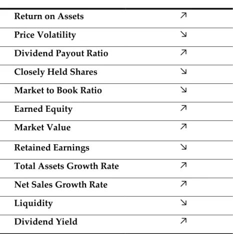
Table 3 - Relation of Explanatory Variables with PDDR
Variable Relation with PDDR Return on Assets ↗
Price Volatility ↘
Dividend Payout Ratio ↗
Closely Held Shares ↘
Market to Book Ratio ↘ Earned Equity ↗
Market Value ↗
Retained Earnings ↘
Total Assets Growth Rate ↗ Net Sales Growth Rate ↗
Liquidity ↘
5. Methodology
In order to estimate ex-dividend stock price behaviour regarding the distributed dividend value, Elton and Gruber (1970) used the arithmetic mean of PDDR:
(9)
where:
: Number of observations
: Closing stock price at the cum-dividend day : Closing stock price at the ex-dividend day : Dividend amount per share
The statistic presented at (4) can otherwise be obtained by calculated the subsequent regression:
, (10)
where is the intercept of the regression, is the random error term, with E( ) = 0 and Var( ) = .
Being able to estimate the price-dividend-to-drop ratio through the own average of price-dividend-to-drop ratios has several estimation issues. Investigators such as Lakonishok and Vermaelen (1983), Eades, Hess and Kim (1984), Barclay (1987), Michaely (1991), Boyd and Jagannathan (1994), Bell and Jeckinson (2002) have pointed out that: the dependent variable does not follow a normal distribution and that the random error, , suffers from heteroscedasticity. The latter problem blossoms from the scaling done by dividends, as the
dividend value varies significantly across firms and industries. Regarding (3), of each stock , , is generated by:
, (11)
where is the random error term with a mean of zero and Var( = . Hence, if we apply and OLS regression to (10), then the residual variance will decrease with respect to dividend yield:
(12)
In order to solve this query, we followed the method utilized by Boyd and Jagannathan (1994), Bell and Jeckinson (2002) and Farinha and Soro (2005). This approach allows us to decrease the weight given to stocks which have low dividend yields and simultaneously high ex-dividend stock price fluctuation. Therefore, rearranging (11) will generate:
(13)
We are now able to estimate PDDR through its regression coefficient slope ( ), using the OLS estimation method:
(14)
However, we believe that the price-drop-to-dividend ratio isn’t only explained by its arithmetical mean. There are several external factors and firm characteristics that may have an impact on the studied variable. Hence,
(15)
where:
: Intercept of the model : Return on Assets : Price Volatility
: Dividend Payout Ratio : Closely Held Shares : Market-to-Book Ratio : Earned Equity
: Market Capitalization : Retained Earnings
: Total Assets Growth Rate
: Net Sales Growth Rate : Liquidity
: Dividend Yield or simply,
(16)
Substituting PDDR at (11) with PDDR at (16) and following the same rationale used from (12) to (13) we estimate PDDR through the OLS model as:
In order to calculate the dividend yield, we use the same approach as
Lakonishok and Vermaelen (1983), Lasfer (1995) and Dasilas (2009), obtaining the instantaneous dividend yield, dividing the dividend value by the stock price at the cum-dividend day .
Regarding heteroscedasticity we will use robust standard errors, although the enhancement that derives from this procedure will result on small efficiency increments, as the estimation was already modified to minimize this issue. We follow the same approach as, for example, Bell and Jeckinson (2002) and Farinha and Soro (2005).
6. Empirical Results
6.1. Regression
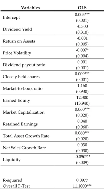
The following Table 4 presents the OLS estimation model results, using robust standard errors:
Table 4 - Regression Model Outcome.
Heteroscedasticity-robust standard-errors in parenthesis. *** p-values <0.01, ** p-values <0.05, and * p-values <0.10.
Variables OLS Intercept 0.003*** (0.001) Dividend Yield -0.300 (0.310) Return on Assets -0.001 (0.005) Price Volatility -0.007* (0.004) Dividend payout ratio 0.001
(0.001) Closely held shares 0.009***
(0.001) Market-to-book ratio 1.160 (0.930) Earned Equity 12.300 (13.940) Market Capitalization 0.060*** (0.020) Retained Earnings 0.040 (0.060) Total Asset Growth Rate 0.060***
(0.020) Net Sales Growth Rate 0.030
(0.030)
Liquidity -0.050***
(0.009)
R-squared 0.0977
The regression model is composed by several variables, ranging from firm financial and operational characteristics, to market related predictors. The OLS regression attempts to clarify which are the significant variables that explain the price-drop-to-dividend ratio, and at what degree they affect it.
Globally, the majority of unit variations that derive from the explanatory variables have a centesimal effect on the dependent variable. Such small impact may be justified by the logarithmic transformation that some predictors were submitted to. However, small fluctuations, especially on stocks with a reduced value, may generate considerable insights regarding dividends and stock appreciation, on an investors’ perspective.
We can infer that according to the model, price volatility is statistically significant at a 10% level, having a negative relation with the explained variable. Closely held shares, market capitalization, total asset growth rate and liquidity are statistically significant at a 1% level. The first three variables are positively related with PDDR, whereas the latter has a negative relation with the dependent variable.
The R-squared of approximately 10%, tells us that the model explains 10% of the variability of the response data, around its mean. The small percentage suggests that other variables should be added to increase the explanatory power of the model, and to test for different possible determinants. Nevertheless, the relationship between the explanatory variables and the dependent variable is significant, hence contributing to the discovery of relevant findings related to the studied issue.
In order to assess the fit of the model, a global significance test was completed. The F-test allows us to conclude whether the projected relationship between the dependent variable and the set of explanatory variables is
statistically reliable. As shown by Table 4, we reject the null hypothesis knowing that the model is globally significant.
6.2. Discussion
The fact that there exists a negative relation between price volatility and PDDR corroborates our expectation. The rationale behind this finding can be rather simple. The higher the volatility of a stock price, the more uncertain its movements become. Higher uncertainty and higher risk associated to a stock price fluctuation will obviously have an impact on cum-dividend and ex-dividend prices, as investors that constitute the market will react to these movements. The higher the volatility the further the fall of the stock’s price to the dividend value.
Closely held shares and PDDR have a positive relation, contrary to our expectations. A higher percentage of closely held shares would suppose a lower price-drop-to-dividend ratio, as managers would have more incentives to invest on non-value-maximizing opportunities, hence retaining shareholder investments for personal benefits, as studied by La Port et al (2000). We suggest that future research regarding ownership and agency models is done in order to better understand its predictable power and reasoning, when opposed to explaining the price-drop-to-dividend ratio.
A positive relation was obtained between market value and PDDR, validating our prediction. We can also try and explain this positive relationship taking in count the importance that market capitalization has, as a proxy for the company’s size. DeAngelo, H., DeAngelo, L. and Stulz (2004), highlight that the bigger a firms’ size, the higher the probability of paying dividends. The bigger the market capitalization of a firm, the bigger its size is in an investor point of view and the greater the capacity of its stock prices to appreciate after the
ex-the company has a solid position on ex-the market, or is growing to achieve it, showing that the improvements at an operational level are being reviewed positively by the market. Hence, the bigger the market capitalization is, the closer the fall of the stock’s price to the dividend value will be.
Total asset growth rate has a positive relation with PDDR, which also confirms our prevision. The fact that a company has a growing total assets rate over the years, has a similar effect to investors, as does a continuous market capitalization growth have. A positive total assets growth rate may lead us to consider that a company is in need of expanding or reinvesting its assets, due to business level improvements. The higher the rate is, the bigger the growth perspectives of the company are. That being said, higher total assets growth rate will lead to a closer fall of the stock’s price considering the dividend value.
The explanatory variable liquidity has a negative relation with the PDDR. In order to attempt to explain this relationship we can argue that a stock price with higher liquidity is easily and more transactional than a low liquidity stock. This high transactional characteristic increases the likelihood of transaction numbers, making it harder for the market and investors to anticipate its daily closing price, making its fluctuation more unpredictable. Such stocks may be more exposed to price volatility than low liquidity stocks, that trade at a lower speed rate, and that on average have a more stable price. Therefore, the higher the stock liquidity the further the fall of the stock’s price from the dividend value.
The remaining predictors are not statistically significant considering the chosen sample. An investigation using the same explanatory variables, but in a different market, is suggested in order to analyse the significance and
Surprisingly, the dividend yield is not statistically significant on the presented model, nor does it relation with the explained variable match what we expected. Such outcome may have been originated by the great variability within the own explanatory variable. The fact that this regression model uses a lot more variables than other models which include the dividend yield may have also contributed to the presented outcome.
Return on assets has a negative relationship with the dependent variable, although our expectation relied on a positive association. Fama and French (2001) and DeAngelo, H., DeAngelo, L. and Stulz (2004), conclude that profitability affects dividend policy. DeAngelo, H., DeAngelo, L. and Stulz (2004), state that the likelihood of a firm paying dividends is positively related with its profitability, using ROA as a proxy. However, due to the logarithmic transformation that the variable went through and perhaps the unfavourable market conditions that characterize the studied period, (where the subprime crisis took place) the output wasn’t as expected.
Dividend payout ratio has a positive relation with PDDR although not statistically significant. According to Lintner (1956), an ideal target ratio predicts future profits, and is based on industry growth perspectives, favourable access to markets, and other variables which are taken in consideration in order to build the perfect payout ratio. It would seem reasonable that the amount of dividends distributed would help explain the fluctuation of stock prices at the ex-dividend day, and narrow the fall of the stock price in comparison to the dividend value. However, as it has been showed, closely held shares contribute to the formation of a perfect dividend payout ratio [according to Rozeff (1982)], are statistically significant contrarily to the ratio as a whole.
Market-to-book ratio has a positive relation with the explained variable, not following what we had previewed. DeAngelo, H., DeAngelo, L. and Stulz
(2004) findings relate the likelihood of paying dividends to growth opportunities in an opposite way. Hence we considered the relation of this explanatory variable to be negative in respect to PDDR, as MTB was a proxy for investment opportunities. In such cases, a firm would prefer to retain its profit, not distributing dividends. Such outcome might once again be related to the change in the final values, which come from the logarithmic change to correct for skewness issues.
A positive relation is observed with the dependent variable and earned equity. The variable is not statistically significant, however, DeAngelo, H., DeAngelo, L. and Stulz (2004) find that earned equity is positively related with the likelihood of paying dividends. Nevertheless such analysis was restricted to nonfinancial and nonutility firms, which could skew the obtained results. The cause for statistical insignificance may derive from the fact that our sample considers all types of firms.
Retained earnings also have a positive relation with the explained variable, not validating our prediction. Being part of several ratios, including earned equity, retained earnings may provide investors with insights at operational level, allowing for a better understanding of a firm’s future investment objectives. Yet, as shown before, less distributed earnings may originate a further drop of the stock price when related to the dividend value. This was not the case. The cause for the switch of the expected sign of the relation between explained and explanatory variables may be once again explained by the skewness correction, as the sign of small logarithms numbers is inverted with the transformation.
Net sales growth rate, used by DeAngelo, H., DeAngelo, L. and Stulz (2004) as a proxy for growth, has a positive relation with PDDR, corroborating our prediction. The fact that this growth rate has the same relation sign with the
significant, suggests that future research comparing both similar rates with the explained variable is developed, in order to better understand the origin of its insignificant result.
7. Conclusion
This study was directed at the UK market and had as main goal, the investigation of which are the determinants of the ex-dividend day price anomaly. The outcome of the investigation allowed us to conclude that on average, the stock price at the ex-dividend day fell 55% of the dividend amount. Therefore, corroborating other studies that also identify the presence of an anomaly at the ex-dividend day.
It is interesting to observe that some variables which are taken in consideration by managers when a dividend distribution is pondered, are also relevant when it comes to the explanation of the ex-dividend day anomaly. We observed that variables such as market capitalization, total assets growth rate and closely held shares, have a positive relation with the price-drop-to-dividend ratio, and are explanatory variables of the presented anomaly. Other determinants such as price volatility and liquidity have a negative relationship with the explained variable.
As in the majority of investigations, some limitations have arisen that however, didn’t compromise the study’s results. For simplicity purposes, we only considered the last yearly value of ex-dividend prices. By consequent, we also considered the yearly average market capitalization and not the average market capitalization ate the ex-dividend day.
Hence, we propose that in similar future research, all the ex-dividend dates are taken into count. It would be interesting to test the same variables at
to suggest the use of other markets for determinants investigation, in order to validate whether or not the results presented in this study are maintained if market characteristics change.