The effects of income and public redistributive policies on income poverty control : a stochastic frontier approach for the EU 28

(1)

The Effects of Income and Public

Redistributive Policies on Income

Poverty Control

A Stochastic Frontier Approach for the EU 28

Trabalho Final na modalidade de Dissertação apresentado à Universidade Católica Portuguesa para obtenção do grau de mestre em Business Economics

por

Miguel dos Santos Rodrigues

sob orientação de

Leonardo Costa

Católica Porto Business School Abril de 2017

(2)

(3)

Acknowledgements

I would like to extend my sincere gratitude to Professor Leonardo Costa, whose guidance, knowledge and dedication proved unmatchable throughout our work together.

I would also like to thank my family and friends, whose support proved to be unconditional and immense, not just in this process, but in everything I have done.

I cannot help but to thank João Rema, for the daily motivation, high hopes and stakes placed in me, and to Jorge Castro, whose rare talent to turn long absences into meaningful presences can never go unnoticed.

Finally, to my dear friend João Gama, the best team player there ever was, whose daily display of leadership, courage and perseverance are the very definition of inspiration, today and every day.

(4)

(5)

Abstract

Income inequality, including income poverty, has been a major source of debate and concern in our world. In the last decades, inequality has been increasing in richer countries. The aim of this research is to explain and compare income poverty and/or its control in the European Union 28 Member States, during the crisis years (2007-2013).

We use Schmidt and Sickles (1984) time-invariant inefficiency model to estimate a single equation stochastic production frontier model and derive inefficiency measures. The output and inputs of the model are respectively the control of poverty, per capita GDP, and per capita redistributive policies (total public spending on Education, Healthcare, and Social Security, per capita). The estimated frontier mirrors a Kuznets’s surface with two input variables, allowing to derive the latter.

Results show that per capita GDP and per capita redistributive policies produce a positive effect on controlling income poverty. Results also show that the most efficient Member States in controlling poverty inequality are not necessarily the wealthiest ones.

Keywords: Income poverty control, Public redistributive policies, Stochastic production frontier analysis, Kuznets surface

(6)

(7)

List of Tables

Table 1 - Descriptive statistics for the output and inputs ... 28 Table 2 - Table 2: Inputs Coefficients, Standard Errors, t-statistics, significance and confidence interval ... 31 Table 3 - Eu Member States ranking in efficiency, per capita GDP and public redistribution policies expenditure ... 32 Table 1A - Average raw data per Member State ... 41 Table 2A - Average rankings of Member State in terms of efficiency, poverty control, per capita GDP, and per capita redistributive policies ... 42 Table 3A - Average raw data per Member State ... 43

(9)

Introduction

Throughout history, inequality between households and poverty have been the object of reflection and reform. Income inequality, the gap between “the poor” and the “wealthy” and whether the existence of such a gap may be reduced has been the work of countless authors in economics. Classical economists like Thomas Malthus, David Ricardo, and John Stuart Mill, and contemporaneous economists like Simon Kuznets, Anthony Atkinson, Amartya Sen, and Thomas Piketty, to name just a few, have addressed this problem.

Income poverty is one of the dimensions of income inequality. The object of this research is the control of income poverty by the European Union 28 (EU 28) Member States during the crisis years and the effects and efficiency of per capita income and of per capita public redistributive policies employed by the Members States. For instance, the EU 28 Member States spend about 26,4% of their GDP in redistributive policies such as Education, Healthcare and Social Security. Therefore, studying the efficiency of these protection mechanisms in effectively diminishing income poverty is of paramount importance.

In the specific case of the EU 28, where this study focuses, the welfare state is enshrined in the European Social Model, which entails the above policies: a public or state-funded system of universal education, healthcare and social security that protects those who are unemployed, as well as the elderly. There are limits to the comparisons and parallels we can establish between countries, given that each system will differ, even if slightly, compared to others. This applies to every European country in each of the three vectors mentioned above. In recent years however, the European Social Model has pretty much been under siege by austerity policies, which, according to European Institutions, are driven forth as a way to mitigate the effects of the financial crisis and balance Member

(10)

States government budgets, while also promoting growth. The economic and financial effects of such policies that required severe budget restraints, especially for countries under bailout programs (e.g. Portugal, Greece, Ireland, Cyprus), is debatable. What is clear is that for countries that applied harsher austerity policies, the risk of poverty and social exclusion sky-rocketed. In Greece, 35,7% of the population was at risk of poverty or social exclusion in 2015 (from 28,1% in 2008). In Spain, the risk of poverty in 2015 was of 28,6% (from 23,8% in 2008). This seems especially true for countries that went through the harshest cuts in their social protection mechanisms.

In this research, using panel data from the European Union 28 Member States during the crisis years, a stochastic production frontier was estimated, based on the model by Schmidt and Sickles (1984) with time-invariant inefficiency. The output of the production function is the control of poverty and the inputs per

capita GDP and per capita public redistributive policies (Education, Healthcare,

and Social Security per capita spending). The estimated stochastic production function mirrors a Kuznets Surface based on income poverty and with two inputs. The research allows benchmarking the position of each Member State towards the production frontier.

The topic of inequality has pretty much dominated both the media and economic attention in recent times, sparkling meaningful debate that departed from the work of Piketty (2013), but also taking over the campaigns and promises on the political landscape. Regardless of how many studies seem to exist on the matter, the question of why some countries fare so much better than others in fighting income inequality remains. Until the work of Piketty (2013), the dominant contemporaneous economic perspective on this matter was handed out by Kuznets (1955).

What can be done about inequality? Again, multiple authors have laid out the groundwork for answering this question. Piketty (2013) has very much put an

(11)

emphasis on a joint fiscal effort, with worldwide coordination, as an attempt to tax higher incomes wherever they are held and, thereby, slow down or even reduce inequality.

In this research, we take into consideration the causes for income inequality listed above, while addressing income poverty, and public redistributive policies followed by European Member States to tackle income inequality and poverty.

The study unfolds as follows. After this introductory chapter, chapter 2 provides the literature review where: i) we provide a deeper insight into income inequality and poverty in developed countries, the Kuznets Curve and its extensions; and ii) we justify the choice of Stochastic Frontier Analysis and describe the use of it by other authors in analyzing and benchmarking the productivity and efficiency of the public sector and policies. In chapter 3, the stochastic production frontier model of time-invariant inefficiency by Schmidt and Sickles (1984) is explained in further detail, alongside the data collected and the estimation itself. Chapter 4 encompasses the results obtained with this model and its discussion. Finally, chapter 5 closes with the conclusion itself.

(12)

(13)

Chapter 2 Literature Review

2.1 Inequality and poverty in developed countries

What are the causes and consequences of high and rising income inequality? In her Keynote Address at the 69th_{UN General Assembly, Gornick (2014)}

provided answers to these questions. Concerning the causes, globalization and increasingly open markets seem to raise income inequality, this being the case for the most open and economically liberal countries of all, the United States of America and the United Kingdom. The access of the public to knowledge and education also seems to be one determinant factor when it comes to income inequality and it is also one we consider in this paper. Redistribution factors and demographics are also to be accounted for, as redistribution systems based on taxes seem to be failing at some point in reducing the ever-widening gap between lower and higher incomes. Furthermore, the increase in one-adult households and the emancipation of women around the world seems to be causing an impact. Finally, other factors like the decreasing unionization of workers across the globe and the increasing financialization of the economy as a whole seem to be playing an important role in the increase of inequality.

In what refers to the consequences, Gornick (2014) points out that rising inequality is often correlated with rising rates of poverty, which is a synonym to say that the poor may be getting even poorer. Needless to say that his has extremely harsh negative consequences for families, communities and countries as a whole. There is also an argument for economic mobility, which is found to be depressed by elevated levels of inequality. This is particularly relevant as

(14)

economic mobility is often seen as an indicator for openness and opportunity. Some authors go as far as to say that elevated levels of inequality may even damage economic growth itself. Stiglitz (2012) argues that a too unequal distribution of income will ultimately depress demand, as people with higher incomes can only consume so much even when maximizing their own utility. Finally, the political issue is one that is relevant to analyze, as evidence has shown that the views of those who are wealthier tend to have more influence in the outcomes of the democratic process. This is, in itself, a distortion of democracy as an ideal where each human enjoys equal rights, voting rights included.

Several other authors have dedicated themselves to this study and, more importantly, their results converge. Atkinson (2015) identifies factors that cause inequality, especially in developed countries, such as globalization, technological change, growth of financial services, changing pay norms and contracts, a reduced role of trade unions and the scaling back of the redistributive tax-and-transfer policy.

In spite of the existence of an agreement on what the causes and consequences of inequality may be, our research is focused in one expression of income inequality in particular: income poverty. In that sense, one should consider exactly how income poverty and inequality are related, as they are not one and the same, despite being heavily correlated.

Bourguignon (2003) called it the Growth-Inequality-Poverty Triangle and sought to explain its interactions. First and foremost, one should not consider growth without considering distribution. On one hand, it is true that economic growth is a necessary condition for reducing income poverty, provided that income distribution remains more or less stable (Dollar & Kraay, 2001). But what happens when it does not? Bourguignon (2003) has shown that a simple shift in inequality as measured by the Gini coefficient could totally overhaul the poverty reduction targets for a given period of time. This means that if wealth distribution

(15)

structure shifts towards “those at the top”, poverty elimination becomes very much a lost cause. The reasons for changes in distributions are unclear, however, as the study has shown that they are essentialy country-specific. Finally, the study shows that in some cases, extreme poverty and inequality could actually offset economic growth as a whole. Therefore, while it is still debatable whether or not inequality is a by-product of growth and whether or not some degree of it is desirable, it is now clear that poverty is not only to be concerned about by moral reasons, but also by the dangers it poses for the economy itself.

Finally, in developed countries like the European ones, inequality seems to behave in a different pattern when compared to other developed countries like the United States. In Europe, income inequality is felt essentially between Member States, whereas the United States, inequality is essentially internal to each State and doesn’t seem to have stark geographic differences (Galbraith, 2009). We expect the same pattern to hold in what refers to income poverty. However, in this research we address income poverty within each Member State of the EU 28 and compare these Member States.

2.2 The Kuznets Curve

The estimated stochastic production frontier of our study is, in itself, a mirror version of a Kuznets Surface. The surface incorporates not only per capita income as an explanatory variable but also per capita public redistributive policies (Healthcare, Education, and Social Security spending, per capita).

Kuznets (1955) proposal was that income inequality would seemingly increase alongside economic growth, only to decrease afterwards, in an inverted U-shaped curve. The explanation for the matter was the fact that people moved from rural (poorer) to urban, industrialized areas, with higher incomes. This

(16)

would imply an increase in income inequality in the first section of the data, where there are still many workers employed in agricultural activities and a posterior decrease, as they migrate towards urban centers. In this case, income inequality itself would increase among those at the bottom as the agricultural workers would maintain their lower incomes and the “new” industrial workers would see their incomes increase. This perspective, however, has severe limitations regarding evidence and/or the narrow statistical basis that supports it, as the years that Kuznets took, into his own sample, only refer to the first half of the twentieth century in the United States and United Kingdom.

More recent studies, however, have been critical of Kuznets’s perspective, the most famous being Piketty’s (2013) study. His position and study support that Kuznets inverse U-shaped curve was comprised in a time period, after which inequality seemed to increase once again, shaping into an N-shaped curve (see Piketty (2013) for the US curve and Rafecas (2010), for the Portuguese curve).

Piketty (2013) argues that the evolution observed by Kuznets was most likely not structural or even fixed, but rather that it was incidental in that given time period.

Other authors have come to criticize Kuznets’s perspective for many reasons, the most common being the scarcity of data used in the study as well as the time period itself. After all, we’re considering a time period that encompasses the Great Depression, two World Wars (and the taxes that were imposed to finance war expenses). It would be very surprising if all of these events hadn’t dealt a major blow to capital owners, such as pointed out by Lyubimov (2017).

Interestingly, despite being hard to prove, Kuznets’s theory went uncontested for several decades. In fact, as pointed out by (Gallup, 2012), not a single author at the time tried to pursue the same method as Kuznets had. Examples include Kravis (1960), Ram (1988), Huang and Lin (2007), among others. Therefore, both defenders and critics lacked the empirical evidence to prove Kuznets to be

(17)

wrong, until Piketty decided to pursue the same method. After Piketty however, more works were developed using the Kuznets curve. For instance, Rafecas (2010) mimicked Piketty’s (2001) study for the Portuguese case, creating a comprehensive analysis on the phenomena of inequality since 1936 to the present day. This proved particularly harsh in the Portuguese case, not just because of the socio-political transformations of the regime, but also because of the fiscal transformations at the time. In Portugal, only in 1929 was a tax over income effectively enforced, after the shift in political regime. This tax reform endured until 1989 where the new constitution and the democratic regime laid the foundations for a new tax reform. These two shifts also put of the method itself to the test. Both Piketty (2001) and Kuznets (1955) used data of tax returns to estimate the amount of wealth held by high income individuals. Rafecas (2010) called it Top Income Shares (TIS) and followed a similar path for Portugal.

Rafecas (2010) study for the Portuguese case shed light on some interesting conclusions. Apparently, TIS suffered a severe drop during and after World War II, only to begin rising once again afterwards, recovering its pre-war levels in the nineteen fifties. It’s interesting to see that for the top decile of the population, even though the TIS decreased after the revolution period (most likely due to nationalizations), this decrease is nowhere near as deep as, for instance, the one caused by WWII. Which suggests that the Carnation Revolution wasn’t as damaging for wealthy individuals as it may have seemed at first.

Extensions

Because of its properties related to economic growth, studies that sought to mimic Kuznets (1955) study to other areas have surged, such as Kuznets Curves for Environment or Healthcare.

(18)

Initially, the inverse U-shape provided a tempting shape to relate economic growth and environment. Since initially societies rely heavily on agriculture, the damage to the environment would be minimal. As societies grow industrial, such environment would deteriorate. However, from a certain level of per capita income onward, people would start feeling other necessities as essential, like clean water and clean air and, therefore, be willing to pay for these conditions to be fulfilled, leading to a decrease in pollution levels and, ultimately, to an inverse U-shaped curve (Yandle, Vijayaraghavan, & Bhattarai, 2002). Tempting as it may be, the same study by Yandle (2002) has shown that although this scheme resembles the evolution of western societies, it does not apply to every country, neither does it apply to every pollutant agent in an identical fashion.

Costa-Font, Hernandez-Quevedo and Sato (2017) attempted to develop a Kuznets Curve applied to healthcare, that related healthcare-related inequalities and economic growth. In this case, however, the data seemed to fit a Kuznets Curve for certain degrees of per capita GDP.

In conclusion, it seems that it is possible to use the shape described by Kuznets (1955) in several areas. However, just like in income inequality, the shape itself seems to be restricted to some factor or time-period.

2.3 Efficiency and Productivity Analysis

Productivity and Efficiency

First and foremost, the path this study took lead us to the analysis of the concepts of productivity and efficiency, which despite being often used indiscriminately, are far from identical concepts. Vincent (1968) defined

(19)

productivity as the ration between production and the “factors” that made it possible. Later, the definition evolved into the ratio between all outputs and all inputs (Lovell, 1993), that is, Total Factor Productivity (TFP). Besides efficiency, other factors affect the TFP, for instance, technical progress.

Most efficiency-related issues are directly connected to ways or methods to maximize it, which leads us to the concept of production frontier. In a simpler fashion, a production frontier would be a collection of all the inputs combinations that, when used, lead to a maximum output. With technical progress, the production frontier moves up increasing TFP. Increasing efficiency also increases TFP.

Several authors have sought and managed to deepen the concept of efficiency. The first and most famous evolution was the concept of technical efficiency (Koopmans, 1951), which stated that an input-output vector would only be considered efficient if diminishing or increasing a given input/output was followed by a proportional increase or decrease in its respective input/output.

Farrel (1957) drove another expansion to the concept of efficiency proposed by Koopmans (1951), by addressing the idea of allocative efficiency. Such is based on the idea that a given process’s efficiency should not be based only on whether the selected combination of inputs ensures the maximum output, but also on whether a given combination of inputs ensures the minimum cost for a given level of production. Farrel (1957) is not referring to production frontiers, in which only technical efficiency applies, but to cost frontiers, where efficiency can be decomposed into technical efficiency and allocative efficiency. The same happens with revenue and profit frontiers.

The next sections of this chapter will discuss a few methodologies for estimating efficiency and productivity. We will focus this discussion specifically on Stochastic Frontier Analysis (SFA) and on Data Envelopment Analysis (DEA), the two most popular methods.

(20)

DEA and SFA

DEA is a non-parametric method for evaluating the efficiency of Decision Making Units (Charnes, Cooper, & Rhodes, 1978). Throughout time, several extensions have been added to the DEA methodology, such as the possibility for variable returns to scale, proposed by Banker, Charnes and Cooper (1984). Both DEA and its extensions work in an analogous way, as they evaluate Decision Making Units (DMUs), identifying a group of DMUs with higher efficiency, which is to say, with a better combination of inputs to produce a given amount of output. Afterwards, the model establishes a ranking between the remaining DMUs and the ones with the “best practices” in the group.

For the estimation of productivity, DEA allows for the construction of a Malmquist Index. This index will essentially be used to compare the production technologies of two different DMUs, allowing for the calculation of technical and efficiency changes (Färe, 1994).

The second method, the one we use in this study, is SFA. It was first proposed by Aigner, Lovell and Schmidt (1977). Stochastic production frontier models, in particular, try to define a frontier where production of any level of a given output is maximized, by considering one vector of inputs and a technological factor (Kumbhakar, 2000). The method itself is defined as stochastic, rather than deterministic, since it encompasses a random variable that captures statistical noise. The main advantages of this method comprise take into account statistical noise present in the samples and to allow the use of more traditional hypothesis testing (Coelli, et al., 1998).

As for calculating and estimating TFP using SFA, one answer is provided by Kumbhakar and Lovell (2000), where the authors propose a quantity-based method, consisting of the estimation of a production frontier where the

(21)

magnitude of change is then calculated and split according to its various identified sources: a technical change component, a returns-to-scale component and a technical efficiency change component (Aguiar, Costa, & Silva, 2016).

When selecting one of the two methods, DEA or SFA, the comparison between the two is very much based on what tradeoffs are possible for the data one is using. For instance, in the case of DEA, no restrictive assumptions about technology have to be made, except about convexity. It is a nonparametric approach. SFA is a parametric approach, as it imposes a functional form. However, the functional form can be flexible.

Furthermore, because DEA requires no distributional assumption about efficiency or stochastic specification is imposed, all variation between DMUs is handled as inefficiency while this is not the case with SFA (see Kumbhakar & Heshmati, 1996).

SFA and Public Policies

Although being a novelty the use of SFA in estimating a production function having as the output “Income Inequality Control” and as inputs per capita income and per capita public redistributive policies, mirroring a Kuznets Surface, the use of SFA in the evaluation of public policies is far from new. SFA has become a regular method for evaluating the efficiency of public services or policies. In Portugal, for instance, Pereira and Moreira (2007) used SFA to analyze the results of the Secondary Education. Interestingly, because in Portugal access to higher education lingers highly on exam results in secondary schooling, they sought to investigate which factors in the education system were helping produce these results, good or bad. For their study, they used the Average Scores on National exams as the single output, whereas the considered inputs were the Number of

(22)

Size and two dummy variables, one for Private Schools and another for a specific regime of tutoring called Ensino Recorrente. Furthermore, three environmental variables regarding Time, Parental Education and Living Standards were added. The results themselves were very interesting, revealing a high degree of technical inefficiency. The study has shown that for the level of employed inputs, the output (grades) could be 10 to 20% higher. It has also shed light to other conclusions, such as the fact that teacher seniority seems to be more important than the number of teachers per 100 students employed. This is obviously the kind of information that allows ministries and legislators to make more informed and effective decisions and it sets out a perfect example of how SFA could be used to evaluate public policies.

The use of SFA has also been extended to other areas of public policies, such as healthcare. Ogloblin (2011) used SFA as a means to extend an already existent study by the World Health Organization. The purpose of this analysis was to evaluate the efficiency of healthcare systems across countries. For that objective, the model used Healthcare Adjusted Life Expectancy. As for the inputs, the model used total expenditure on health care per capita in international purchasing power parity (PPP in dollars), the average years of schooling of population over 25 years old - as higher educated individuals are less prompt to take risk behaviors – the percentage of smokers among young adults and alcohol consumption over young adults.

The process followed through with a second stage regression, as an attempt to explain the observed inefficiency. In this case, inefficiency was regressed on the Gross National Income per capita, the GINI coefficient, the Public Healthcare Expenditure as a percentage of total healthcare expenditure and the “Out-of-pocket” healthcare expenditure as a percentage of total healthcare expenditure.

Again, this has proven useful in evaluating public policies, as the study has shown a clear direction to head for. The results implied that healthcare systems’

(23)

inefficiency was inversely correlated with per capita income. It has also shown that countries with lower inefficiency scores were the ones that allocated higher slices of public and out-of-pocket budget as a percentage of total healthcare expenditure. This seems to suggest, among other things, that countries that use private insurance systems are less efficient in addressing healthcare policies.

(24)

(25)

Chapter 3 Empirical Model

3.1 Efficiency and Productivity Analysis

In chapter 1, we set out the purpose of this dissertation as to developing a Kuznets Surface to evaluate the efficiency and productivity of per capita income and per capita public redistributive policies on controlling income inequality and, most specifically, income poverty. In chapter 2, we provided a deep insight of the Kuznets Curve, both in its original state and the extensions that were created to explore other phenomena that were, as we saw, not necessarily related to income inequality. Moreover, insight on both parametric and non-parametric methods available for the type of study that was being developed, namely DEA and SFA, were explored.

In this chapter, we’ll address the production of a single output (inequality control) using two different inputs: per capita GDP and per capita public spending on redistributive policies (Education, Healthcare, and Social Security spending,

per capita). The objects of this study are 27 European Member States of the EU 28

(Croatia was excluded as an outlier of the sample). Member States of the EU 28 are seen as DMU’s producing an output (income poverty control) and using two inputs (per capita income and per capita public redistributive policies). The distance between the observed output and the potential output reflects a country’s level of technical inefficiency. With time-invariant inefficiency models, as the one by Schmidt and Sickles (1984), the frontier itself is defined by the most efficient unit across the entire time period. In addition, all inefficiency or the distance from the frontier is assumed to be technical inefficiency and constant for each DMU in the period.

(26)

For the remainder of this chapter, we will provide a brief summary of the model by Schmidt and Sickles (1984). Afterwards, we will go through the estimation equation and its parameters.

3.2 The Schmidt and Sickles (1984) Model

Schmidt and Sickles (1984) model is given by:

𝑦_𝑖𝑡 = 𝑎_𝑖+ 𝑥′_𝑖𝑡𝛽 + 𝑣_𝑖𝑡 (3.1) with 𝛼𝑖 = 𝛽0− 𝑢𝑖 (3.2)

Where:

• 𝑦_𝑖𝑡 represents the output produced by DMU 𝑖, (with 𝑖 =1,2,…,N) for period ( 𝑡=1,2,…,T);

• 𝑥′_𝑖𝑡 is the (1*k) vector of inputs for the production function associated with the DMU 𝑖 in period 𝑡;

• 𝑎_𝑖 is the fixed effect for DMU 𝑖 in every given period 𝑡,

• 𝑣𝑖𝑡 refers to the random error component, which is assumed to be identically distributed in N(0, 𝜎𝑣2).

First and foremost, the fixed effect 𝛼𝑖 is equal to the difference between the constant 𝛽0 and the technical inefficiency term 𝑢𝑖. As a consequence, this model takes the assumption that both 𝑢𝑖 and 𝑎𝑖 are time-invariant and to be estimated simultaneously with 𝛽.

(27)

After obtaining the estimates of 𝛽̂ and the fixed effect 𝛼𝑖 , we can estimate 𝑢̂𝑖 as:

𝑢̂𝑖 = max(𝑎̂𝑖) − 𝑎̂𝑖 ≥ 0, 𝑖 = 1,2, . . . , 𝑁 (3.3)

What this means is that for each time period 𝑡 technical inefficiency is calculated in relative terms compared to the most efficient DMU, in this case, Member State, across the whole time period. Finally, we can obtain an estimate of technical efficiency by country:

𝑇𝐸𝑖 = exp( −𝑢̂𝑖) (3.4)

3.3 Data and Treatment

The data used in this study was collected for the EU 28 Member States in the 2007-2013 period. The data used was collected from Eurostat and data publications by the European Commission, for a grand total of 189 observations (after excluding Croatia as an outlier). The years selected for the sample were meant to capture the effects of the crisis in Europe.

The selected output variable is the control of income poverty in percentage of total population. This variable is obtained by subtracting to 100% the percentage of population with income below what is defined by the EU criterion as the at-risk-of-poverty-rate1_.

The input variables used were per capita GDP at Purchasing Power Parities for ESA (European System of Regional and National Accounts) 2010 aggregates and

per capita Public Redistributive Polices (Education, Healthcare, and Social

1_{The at-risk-of-poverty rate is the share of people with an equivalized disposable income (after social transfers)}

(28)

Security, altogether, spending, per capita). The choice of these two inputs reflects the purpose of assessing the impact of per capita income and of per capita public redistributive policies in income poverty control.

Table 1 below describes the average sample raw data. Table 1A, in the Appendix, yields the average raw data per Member State.

Variable Obs Mean Std. Dev. Min Max

Poverty Control 189 75,44127 8,488778 39.3 86.1

Per capita GDP 189 98671,96 41071,4 41000 264000

Per capita Redistributive Policies

189 27029,2 13882,47 6396 76560

Table 1: Descriptive statistics for the output and inputs Source: Eurostat

The following treatment has been given to the data. The log of both inputs has been taken. The output and the log of both inputs has been normalized into indexes using the following formula:

𝑥𝑖𝑛𝑑𝑒𝑥_𝑖𝑡 = 𝑥𝑖𝑡−min (𝑥𝑖𝑡)

max (𝑥𝑖𝑡)−min (𝑥𝑖𝑡)

(3.5)

3.4 Estimation

The production function considered in this study is the following quadratic flexible functional form2_:

2_{On a final note, the choice of the quadratic flexible functional form production frontier can be explained by the}

specific features of this form, as quadratic functions don’t impose constraints on elasticities of substitution between inputs and output elasticities with respect to any given input are country and time specific, making it very

(29)

𝑦𝑖𝑡 = 𝑎0𝑖+ 𝛽1𝑔𝑑𝑝𝑖𝑡+ 𝛽2𝑠𝑝𝑖𝑡+ 𝛽3𝑔𝑑𝑝𝑖𝑡∗ 𝑠𝑝𝑖𝑡+ 𝑣𝑖𝑡 (3.6)

Where:

• 𝑦_𝑖𝑡 denotes an index of the percentage of population above the poverty threshold for country i in week t;

• 𝑔𝑑𝑝_𝑖𝑡 denotes an index of the log per capita GDP for country i in year t, measured in Purchasing Power Parities for ESA 2010 aggregates; • 𝑠𝑝_𝑖𝑡 denotes the an index of the log per capita Public Redistributive

Policies (Education, Healthcare and Social Security, altogether, spending, per capita);

We started with the more general quadratic function but the coefficients on the squared terms were not significant.

(30)

(31)

Chapter 4 Results

4.1 Empirical Model Estimates

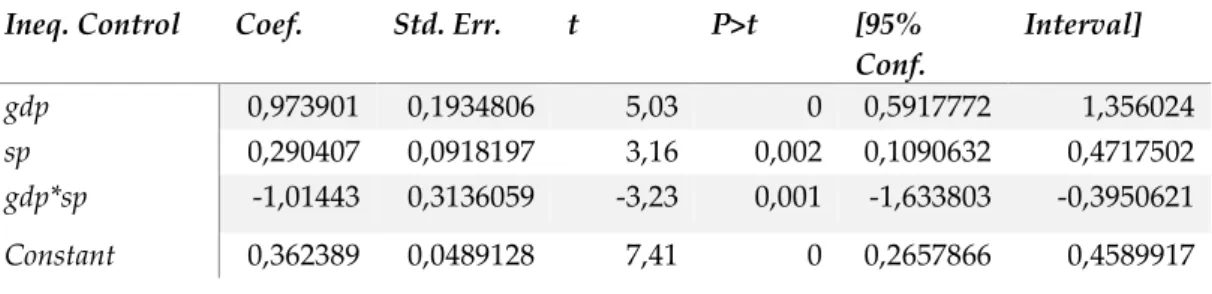
The estimates for the fixed effects quadratic regression Schmidt and Sickles (1984) model were obtained using the software Stata. Table 2 below presents the results of the regression, including coefficient estimates, standard errors, t statistics, p-values, and 95% confidence intervals. Table 3A, in the Appendix, yields the Fixed Effects per Member State.

Ineq. Control Coef. Std. Err. t P>t [95% Conf. Interval] gdp 0,973901 0,1934806 5,03 0 0,5917772 1,356024 sp 0,290407 0,0918197 3,16 0,002 0,1090632 0,4717502 gdp*sp -1,01443 0,3136059 -3,23 0,001 -1,633803 -0,3950621 Constant 0,362389 0,0489128 7,41 0 0,2657866 0,4589917

Table 2: Inputs Coefficients, Standard Errors, t-statistics, significance and confidence interval;

All coefficients are significant, at a 1% level of significance. The control of income poverty increases linearly with per capita log of GDP and per capita log of public redistributive policies.

The negative sign of 3 says that inputs are substitutes, leading us to the

conclusion that if per capita GDP drops, per capita redistributive polices spending may increase in order to keep income poverty control constant. This also implies that if per capita GDP increases, a lower level of redistributive policies spending is required to maintain the same level of poverty control. Both conclusions are consistent with the data.

(32)

The partial elasticities for both factors point to a reduction of income poverty, which is consistent with the obtained coefficients. In the case of per capita GDP, a 1% increase in the log of per capita GDP will lead to a 0,29% increase in poverty control. In the case of redistributive policies spending, a 1% increase in the log of

per capita Social Redistributive Policies spending will lead to a 0,02% increase in

poverty control.

By adding the partial elasticities, we obtain a scale elasticity equal to 0,215, which is less than 1. That is, the production function has decreasing returns to scale. When increasing both inputs in a given proportion the increase in the output is less than proportional.

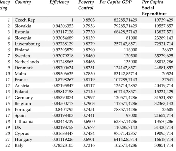
Table 3 shows the ranking of technical efficiencies and the levels of raw output and inputs across Member States. The rankings of output and inputs are provided in Table 2A, in the Appendix.

Efficiency Ranking

Country Efficiency Poverty Control

Per Capita GDP Per Capita

Social Expenditure 1 Czech Rep 1 0,8503 82285,71429 19739,429 2 Slovakia 0,94306353 0,7956 79285,71429 19557,857 3 Estonia 0,93117126 0,7730 68428,57143 13827,571 4 Slovenia 0,93054689 0,8139 81000 23289,143 5 Luxembourg 0,92738129 0,8279 257142,8571 72921,714 6 Finland 0,92393879 0,8290 116000 38632 7 Sweden 0,92079218 0,8460 120500 35279,625 8 Netherlands 0,91248865 0,8466 135000 38013,286 9 Denmark 0,89700624 0,8251 124142,8571 44881,857 10 Malta 0,89506635 0,7850 83142,85714 20524 11 France 0,8798267 0,8119 107285,7143 37541 12 Austria 0,87195847 0,8117 126714,2857 40419,714 13 Poland 0,85812158 0,7140 60714,28571 15224,429 14 Germany 0,85390074 0,7997 120571,4286 31531,857 15 Belgium 0,84500717 0,7903 117571,4286 32363,143 16 Portugal 0,8404795 0,7451 78857,14286 23605 17 Spain 0,83198403 0,7441 97000 21652,714 18 Lithuania 0,82448739 0,6900 63857,14286 13570,286 19 UK 0,82198758 0,7677 110285,7143 31430,714 20 Cyprus 0,81688447 0,7484 97571,42857 19095,714 21 Hungary 0,81119226 0,6901 64142,85714 16618,714 22 Italy 0,78328105 0,7316 102571,4286 30851,714

(33)

23 Latvia 0,77857557 0,6331 57428,57143 11062,571

24 Ireland 0,75308107 0,7304 133000 36140,143

25 Romania 0,73774206 0,5690 49571,42857 8755,8571

26 Greece 0,73242874 0,6957 84571,42857 24413,714

27 Bulgaria 0,6795346 0,5039 45000 8081

Table 3: Eu Member States ranking in efficiency, per capita GDP and public redistribution policies expenditure.

Source: Eurostat

The Czech Republic has been the most efficient Member State and, in this sense, outperformed its European partners. The ranking refers to the efficiency of both income and social redistributive policies in controlling income poverty and not to the level of output nor to the level of inputs, which are also stated in Table 3. For instance, it does not mean that the Czech Republic is the Member State with the higher control of income poverty, although it is (see Table 2A, in the Appendix). It also does not mean that the Czech Republic is the richest country, which is Luxemburg, or the country which puts the most effort in terms of redistributive policies, which is Denmark (see Table 2A in the Appendix). The less efficient Member States are Romania and Bulgaria.

For other Member States to become more successful in managing their income poverty control, a solution would be to understand and approach the practices of the most efficient Member States, namely the Czech Republic.

The results suggest that a high degree of efficiency does not necessarily imply an extremely high per capita GDP and per capita public redistributive policies spending. This is especially true for countries like the Czech Republic or Slovenia, which despite their high efficiency on controlling poverty, are outperformed by far in terms of per capita GDP and per capita public redistributive policies by other Member States. However, we cannot say that per capita GDP and per capita public redistributive policies spending do not play a major part in most cases. This is especially true for northern European Scandinavian Member States, such as

(34)

Sweden, Denmark and Finland, which place themselves in the top 10 for poverty control, efficiency, per capita GDP, and per capita redistributive policies spending. It is also notorious that a few Member State that spend highly in redistributive policies spending have weak results on controlling income poverty. This is especially true for Portugal, Italy, France and Greece. In spite of that, one cannot disregard that the period analyzed in this study was particularly turbulent, particularly for Greece and Portugal. It’s possible that the poor results obtained in this period being very much a reflection of the economy’s performance. However, it is also possible that these results are the reflection of more serious structural problems that should be addressed.

The Portuguese case is an interesting, as Portugal ranks 16th_{in terms of}

efficiency on controlling income poverty and 14th_{in per capita redistributive}

policies spending. However, when we look at the public redistributive spending as a percentage of GDP, Portugal is actually the 6th_{country that spends the most}

in Social Protection. This may reflect a poor allocation of resources, but it may also reflect deeper structural problems such as population ageing and structural unemployment, which may be forcing the social protection expenses in both unemployment subsidies and old-age pensions. It may also reflect the crisis environment, namely, cyclical unemployment and GDP contraction due to the crisis and the way it was managed by the European Institutions. Austerity has not been expansionary in any Member State, particularly in Portugal and Greece, quite the opposite.

(35)

Chapter 5 Conclusion

In this study we used the Schmidt and Sickles (1984) stochastic production frontier time-invariant inefficiency model to analyze the efficiency of each Member State of the EU 28 in managing the control of income poverty, the output, considering as inputs per capita GDP and per capita Redistributive Policies spending (Education, Healthcare, and Social security spending, altogether, per capita), and using a quadratic flexible functional form.

Results show that both per capita GDP and per capita Social Redistributive Policies spending are positively related with income poverty control. Increasing

per capita GDP increases the income poverty control linearly. Increasing per capita

Public Redistributive Policies spending also increases income poverty control linearly. The inputs are substitute and the returns to scale of the production function are decreasing.

These above results pose a strong stance against the austerity policies that were adopted by Member States in the time period in question, which involved essentially cuts to the European Social Model and, therefore, to the Healthcare, Education and Social Security Redistributive Policies that Member States possess, and, simultaneously, recessionary effects over the GDP. Both factors have contributed to an increase of income poverty in the Member States of the EU 28, particularly in Member States subject to the intervention of the Troika.

The mean efficiency for the countries in question is of 85,3% meaning that, on average, European Member States allocate both their per capita GDP and per capita Redistributive Policies Spending in a highly efficient way. The exceptions to this are located essentially on Eastern Europe, outside of the EU-15 area, although

(36)

some of these eastern countries, namely the Czech Republic, are highly efficient in fighting income poverty. The other exception is Greece that, albeit being an EU-15 country, underwent two harsh austerity programs during the period, which may partially explain this result.

The efficient frontier for all years is granted by the Czech Republic. Despite the crisis, the Czech Republic shows a good performance in what concerns to economic growth and employment. These results may be related to the fact Of the Czech Republic not being a part of the Eurozone, which grants it the control of its exchange rate and monetary policies.

Finally, future developments for this study would consist on using different measures of income inequality besides income poverty. Also, it would definitely be useful, for the purpose of policy making, to further separate the impacts of the several Public Redistributive Policies (Education spending, Healthcare spending, and Social Security spending, per capita).

(37)

Bibliography

Acemoglu, D., & Robinson, J. A. 2002. The Political Economy of the Kuznets Curve. Review of Development Economics, 6(2), 183-203.

Aguiar, D., Costa, L., & Silva, E. 2016. An Attempt to explain Difference in Economic Growth - A stochastic frontier approach. Bulletin of Economic

Research

Aigner, D., Lovell, C., & Schmidt, P. 1977. Formulation and Estimation of Stochastic Frontier Production Functions. Journal of Econometrics, 21–37. Atkinson, A. B. 2015. Inequality - What can be done? Cambridge, Massachussets:

Harvard University Press.

Banker, R., A, C., & WW, C. 1984. Some Models for Estimating Technical and Scale Inefficiencies in Data Envelopment Analysis. Management Science,

30, 1078-1092.

Bourguignon, B. F. 2003. The Poverty-Growth-Inequality Triangle. Proceedings

of the AFD-EUDN, (pp. 69-106).

Charnes, A., Cooper, W. W., & Rhodes, E. L. 1978. Measuring the efficiency of decision making units. European Journal of Operational Research, 429-444.

Coelli, T. J., Rao, D. P., O'Donnell, C. J., & Battese, G. E. 1998. An introduction to

Efficiency and Productivity Analysis (2nd ed.). New York, United States

of America: Springer.

Cornwell, C., Schmidt, P., & Sickles, R. C. 1990. Production Frontiers with Cross-Sectional and Time-Series Variation in Efficiency Levels. Journal of

(38)

Costa-Font, J., Hernandez-Quevedo, C., & Sato, A. 2017. A health 'Kuznets' Curve'? Cross-section and Longitudinal Evidence on Concentration Indices. Social Indicators Research, 1-14.

Dollar, D., & Kraay, A. 2001. Trade, Growth and Poverty. Finance &

Development - International Monetary Fund, 38.

Färe, R. G. 1994. Productivity Growth, Technical Progress, and Efficiency Change in Industrialized Countries. The American Economic Review, 84, 66-83. Galbraith, J. K. 2009. Inequality, unemployment and growth: New measures for

old controversies (Vol. 7). Springer.

Gallup, J. L. 2012. Is There a Kuznets Curve? Working Paper.

Gornick, J. C. 2014. High and Rising Inequality: Causes and Consequence.

General Assembly 69th Session Second Committee General Debate – Ke ynote Address , (pp. 1-14). New York.

Kumbhakar, S. C., & Heshmati, A. (1996). DEA, DFA and SFA: a comparison.

Journal of Productivity Analysis , 303-327.

Kumbhakar, S., & Lovell, C. A. 2000. Stochastic frontier analysis. Cambridge: Cambridge University Press.

Kuznets, S. 1955. Economic Growth and Income Inequality. The American

Economic Review, 1-28.

Lyubimov, I. 2017. Income inequality revisited 60 years later: Piketty vs Kuznets.

Russian Journal of Economics, 42-53.

Oglobin, C. 2011. Healthcare Efficiency Analysis Across Countries: A Stochastic Frontier Analysis. Applied Econometrics and International Development. Pereira, M. C., & Moreira, S. 2007. A Stochastic Frontier Analysis of Secondary

Education in Portugal. Banco de Portugal - Working Paper.

Piketty, T. 2001. Les Hauts Revenues en France au XXè siècle - Inegalités et

Redistributions 1901-1998. Paris: Grasset.

(39)

Rafecas, J. G. 2010. The Evolution of Top Income and Wealth Shares in Portugal Since 1936. Journal of Iberian and Latin American Economic History, 139-171.

Schmidt, P., & Sickles, R. C. 1984. Production Frontiers and Panel Data. Journal

of Business & Economic Statistics, 2, 367-374.

Stiglitz, J. E. 2012. The Price of Inequality. New York: W. W. Norton & Company. Yandle, B., Vijayaraghavan, M., & Bhattarai, M. 2002. The Environmental

(40)

(41)

Appendix

Table 1A: Average raw data per Member State

Country Poverty Control (% Population)

Per capita GDP (€)

Public Social Expenditure (% GDP) Austria 0,811714286 126714,2857 31,88571429 Belgium 0,790285714 117571,4286 27,5 Bulgaria 0,503857143 45000 17,92857143 Cyprus 0,748428571 97571,42857 19,64285714 Czech Republic 0,850285714 82285,71429 23,98571429 Denmark 0,825142857 124142,8571 36,12857143 Estonia 0,773 68428,57143 20,28571429 Finland 0,829 116000 33,34285714 France 0,811857143 107285,7143 34,98571429 Germany 0,799714286 120571,4286 26,15714286 Greece 0,695714286 84571,42857 29 Hungary 0,690142857 64142,85714 25,91428571 Ireland 0,730428571 133000 27,25714286 Italy 0,731571429 102571,4286 30,1 Latvia 0,633142857 57428,57143 19,4 Lithuania 0,69 63857,14286 21,37142857 Luxembourg 0,827857143 257142,8571 28,37142857 Malta 0,785 83142,85714 24,67142857 Netherlands 0,846571429 135000 28,18571429 Poland 0,714 60714,28571 25,1 Portugal 0,745142857 78857,14286 29,92857143 Romania 0,569 49571,42857 17,62857143 Slovakia 0,795571429 72142,85714 24,05714286 Slovenia 0,813857143 83857,14286 29,15714286 Spain 0,744142857 97000 22,4 Sweden 0,846 125285,7143 29,64285714 UK 0,767714286 110285,7143 28,54285714 Source: Eurostat

(42)

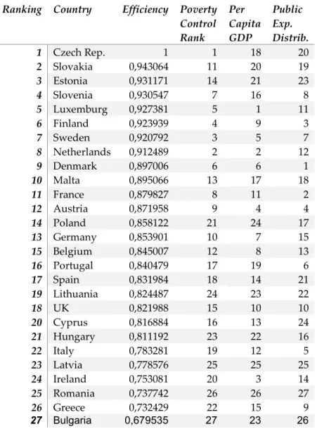
Table 2A: Average rankings of Member State in terms of efficiency,

poverty control, per capita GDP, and per capita redistributive policies.

Ranking Country Efficiency Poverty Control Rank Per Capita GDP Public Exp. Distrib. 1 Czech Rep. 1 1 18 20 2 Slovakia 0,943064 11 20 19 3 Estonia 0,931171 14 21 23 4 Slovenia 0,930547 7 16 8 5 Luxemburg 0,927381 5 1 11 6 Finland 0,923939 4 9 3 7 Sweden 0,920792 3 5 7 8 Netherlands 0,912489 2 2 12 9 Denmark 0,897006 6 6 1 10 Malta 0,895066 13 17 18 11 France 0,879827 8 11 2 12 Austria 0,871958 9 4 4 14 Poland 0,858122 21 24 17 13 Germany 0,853901 10 7 15 15 Belgium 0,845007 12 8 13 16 Portugal 0,840479 17 19 6 17 Spain 0,831984 18 14 21 19 Lithuania 0,824487 24 23 22 18 UK 0,821988 15 10 10 20 Cyprus 0,816884 16 13 24 21 Hungary 0,811192 23 22 16 22 Italy 0,783281 19 12 5 23 Latvia 0,778576 25 25 25 24 Ireland 0,753081 20 3 14 25 Romania 0,737742 26 26 27 26 Greece 0,732429 22 15 9 27 Bulgaria 0,679535 27 23 26 Source: Author

(43)

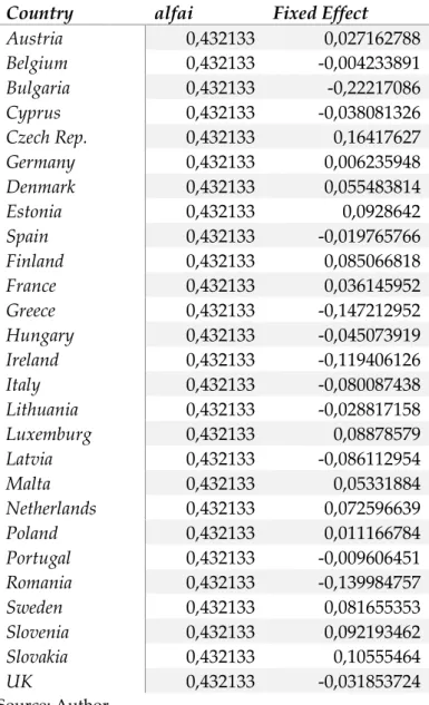
Table 3A – Fixed Effects per Member State

Country alfai Fixed Effect

Austria 0,432133 0,027162788 Belgium 0,432133 -0,004233891 Bulgaria 0,432133 -0,22217086 Cyprus 0,432133 -0,038081326 Czech Rep. 0,432133 0,16417627 Germany 0,432133 0,006235948 Denmark 0,432133 0,055483814 Estonia 0,432133 0,0928642 Spain 0,432133 -0,019765766 Finland 0,432133 0,085066818 France 0,432133 0,036145952 Greece 0,432133 -0,147212952 Hungary 0,432133 -0,045073919 Ireland 0,432133 -0,119406126 Italy 0,432133 -0,080087438 Lithuania 0,432133 -0,028817158 Luxemburg 0,432133 0,08878579 Latvia 0,432133 -0,086112954 Malta 0,432133 0,05331884 Netherlands 0,432133 0,072596639 Poland 0,432133 0,011166784 Portugal 0,432133 -0,009606451 Romania 0,432133 -0,139984757 Sweden 0,432133 0,081655353 Slovenia 0,432133 0,092193462 Slovakia 0,432133 0,10555464 UK 0,432133 -0,031853724 Source: Author

The effects of income and public redistributive policies on income poverty control : a stochastic frontier approach for the EU 28