Bolm Inst. oceanogr., S Paulo, 28(2) : 65- 78, 1979
VERTICAL DISTRIBUTION OF
PARACALANUS CRASSIROSTRTS
(COPEPODA,
CALANOIDEA): ANALYSIS BY THE GENERAL LINEAR MODEL
1ANA MILSTEIN2 , 3
Instituto Oceanográfico da Universidade de são Paulo
Synopsis
The verticaZ distribution of ea0h deveZopmentaZ stage of P~~atanU6 ~~i~~~
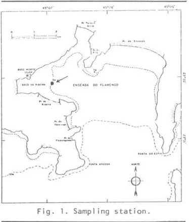
was studied in a shaZZow water station at Ubatuba, SP, BraziZ (23°30'S-45°0?'W). SampZes were coUected monthZy at the surface, 2m andnear bottom ZeveZs. SaZinity, temperature, dissoZved oxygen, tide height, Zight penetration and soZar radiation were aZso recorded. Data were anaZysed by the generaZ Unear modelo It showed
that the amount of individuaZs at any deveZopmentaZ stage is affected diverseZy by hour, depth, hour-depth interaction and environmentaZ factors throughout the year and that these effects are stronger in summer. AU deveZopmentaZ stages were spread in the water coZumn showing no reguZar verticaZ migrations. On the other hand, the n'Ul7Wer of organisms caught in a particuZar hour seemed to dependmore on the tide than on the animaZs behaviour. The resuZts of the present paper showed, as observed by some other authors, the Zack of verticaZ migration of a coastaZ copepod which is a grazer of fine particZes throughout its Zife.
Introduction
Many studies at sea and in 1aboratories have been performed in order to
under-stand and exp1ain the vertical migration of p1ankton, but l i tt1e is known about this phenomenon in sha110w waters. Papers on VM (vertical migration) in
1aboratorie~ have been written by Lewis
(1959), Lance (1962), Enright
&
Hannner (1967), Bjornberg&
Wi1bur (1968), and Grind1ey (1972). Researches on VM at sea, in in1et or sha110w waters, have been worked out by Yamazi (1957), Jacobs(1968), Pi11ai
&
Pi11ai (1973), Daro (1974), Stickney&
Know1es (1975), Furuhashi (1976) and Grind1ey (1977).In Brazi1, besides that of Bjornberg
&
Wi1bur mencioned above, some otherstudies on VM have been performed: on total p1ankton (Moreira, 1976),
1 Thesis submitted to the Instituto
Oceano-gráfico da Universidade de são Paulo, in partia1 fu1fi11ment of the requirements for the degree of Master in Bio10gica1 Oceanography.
2 From September 1977 on, this work was
Hydromedusae (Moreira, 1973), Lu~6e~
6aXOM
(Jimenez, 1976), and C1adocera and Ostracoda (Rocha, 1977) at a 50 m depth station off Santos, and on adu1t P~~a.tanU6
~f.J~M.tJl.Á.,6 at Ubatuba (Mi1stein, in press). .Taking into account the importance of coasta1 waters in the productivity of the seas, the study of vertical distribution of zoop1ankton in sha110wwaters have been proposed. In this paper, the VM of each deve10pmenta1 stage of P~~atanU6
~f.J~f.J.tJl.Á.,6 at a 5 m depth station at
Ubatuba is ana1ysed throughout the year. This species was chosen because i t is one of the most abundant in the tropic and sub tropi c be lts . I t is an indi ca tor of coasta1 waters (Bjornberg, 1963), which can be found a1so in in1et areas. It has been recorded from a1most fresh waters up to marine ones (Sewe11, 1948); Devasundaram & Roy, 1954; Bjornberg, 1963; Teixeira, Tundisi & Kutner, 1965; Tundisi, 1972) and of temperature between 1°C (Anraku, 1964) and about 30°C (Gurney, 1927; Grice, 1960; Bjornberg, 1963; Tundisi, 1972).
sponsored byafellowshipgivenby O.E.A. Material and sampling methods
3 Present address: Museo Nacional de
Histó-ria Natural, Casi11a 399, Montevideo, Uruguay.
Pub.t. n9
453do Inf.Jt.
o~eanog~.da
U6p.
66
Bolm Inst. oceanogr., S Paulo,28(2), 1979
to May 1977) at four to seven weeks inter-vaIs. Each day samples were collected at 06:00, 12:00, 18:00 and 24:00, in three leveIs: surface, 2 m, and near the bottom (3.5 to 4.5 m acccrding to tide).
Each station lasted one hour. From each leveI, Nansen bcttle water saulplcs for dissolved oxygen and salinity aualysis were taken, and 99 f of water (sampled with a 9 f van Dom bottle) were filtered
throughout a 37 micra mesh size net and pr
2-served in neutral formalin 4%. Bottom
Figo 10 Sampl ing stationo and surface net plankton samples were also collected, but were not analysed. Environmental f8~tors were recorded:
light penetration, temperature (with a reversing termometer fi tted to the Nansen bottle), solar radiation, and tide
records.
Dissol ved oxyg~n was ti trated by
Winkler's method and salinity was
measured by conductivity. AlI individu-aIs of
P.
~~~O~~ in the bottle samples were counted, separately each stage.Identification of nauplia was based on Bjornberg's (1972) ~aper, and that of copepodids on Lawson & Grice's (1973). Envi ronment
-Enseada do Flamengo is a sheltered bay, surrounded by high lands and islands, without important fresh water affluents. Semidiumal tides are the principal mixing mechanism with adjacent water masses
(Teixeira, 1973). Waters are
eumixo-haline with temperatures between 20 and 30°C.
The~e are two seasons, not sharply separated. In winter the infloT,y of fres~
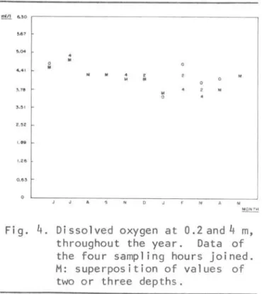
water due to rain are greqter than in summer, and consequently the salinities recorded we"':"e lower; the water column ;n this period was mixed, without strong dissolved oxygen and temperature gradi-ents. In summer bigger differences were found between surface 'lnd bottom records of salinity, dissolved oxygenand tempe,,:,-ature (Figs 2, 3, 4). In the s .~. me area,
similar results wer~ found by Teixeira
">' •• 36,00
[
3.J.60
M
o
3~,20
34.80 • o
34,40
"',00
• •
33,60 o
33.2:0
M
32,80
32.4)
32.00
-•
Fig. 2. Salinities at 0.2 and
4
m, throughout the year. Data of the four sampling hours joined.M:
superposition of values cf two or three depths.MON TH
"''''
"'0... 7
'.04 •
M
O
4 • • 1 M
M M •
•
M M 3,78
M O
3.'1
2 , ~Z
I,ae
1. 26
0,63
O
Fig. 4. Dissolved oxygen at O.2and4 m, throughout the year. Data of the four sampling hours joined. M: superposition of values of two or three depths.
(1973), who also studied other physical and chemical factors, and by Nonato, Miranda
&
Signorini (1974, according to Amaral, 1977). Other detailed de-scriptions of the area are given by Schaeffer-Novelli (1976), Amaral (1977), Fernandez (1977) and Pires (1977).Statistical analysis
The use of the general linear model (Omega) in biology was discussed by Seal (1966) and utilized in marine biology by Buzas (1969, 1971); computacional pro-cedures can be found in BMD ManuaIs (Dixon, 1974) as "General Linear Hy-pothesis". The data were computed in the Burroughs B-6700 Systemof the Centro de Computação Eletrônica da Universidade de são Paulo.
The least squares technique known as regression analysis of a linear model was used. This method seeks to "explain" a single variate in terms of a number of other variables (independent variables and covariables).
If the residuaIs are assumed to have been independently sampled from one normal distribution, their own distri-bution can be assumed to be normal with zero mean (N (0,02
»,
and the "best"numerical values of the parameters of the model will be obtained by minimizing the sum of squares of the residuaIs respect to variation in these parameters (Seal 1966, p. 7).
To be sure that the distributions were normal, standard deviation against mean was plotted for each stage of
P.
67
c.Jl..Ov6.6,úw.6:tJL..L6; each poin t of the gr aphi cs rises from the data of one month. In alI figures these parameters tum out to be linearly proporcional, so that the appropriate transformation for normal-izing the data and stabilnormal-izing the vari-ance is the logarithmic one (Barnes, 1952). To avoid the problem of samples with no individuaIs, log (n+1) was used. The independent variables values of the factorial design (hour and depth) were fixed a priori, and can be con-sidered free of errar.
Mbdel Omega was constructed a priori, taking into account animal densities, environmental variables, depth differ-ences, hour differdiffer-ences, and the inter-action of depth and hour differences. In order to know which parameters are significantly different from zero, model Omega was compared with several more re-stricted omega models. Each of these restricted modeJs were obtained equating a group of parameters of the general Omega model to zero.
A significant effect of a factor means that this factor accounts for atleast part of the variation of the number of animaIs found in the samples, at the sig-nificance leveI considered.
In matrix notation model Omega can be written as
Z' •
Q +IJ
e
Á..jk.(N.q) (q.l) (N.l)
where
x
is the vector ofN
observations,Á..= 1,2,3, 4 hours,
j=
1,2,3 depths,k.=
1,2 replicates (months), Z I is a matrix of instrumental variables and covariables,S
is a vector ofq
parame-ters to "explain" the N observations, ande
is a vector of "errors" or "residuaIs" not accounted for by the model and assumed to be N(O, ( 2 ).Matrix Z' rises from equations on Table I.
The makeup of the columns of matrix Z' is shown in Table 11. Each element of vector Zo is 1, so that, by making each of the other vectors of instru-mental variables sum to zero,
80
be-comes the mean of all observations. Vectors Zl through Z3 account for hourdifferences (line effect in factorial design), vectors z~ and Zs account for depth differences (colunn effect); interaction vectors Z6 through Zll were
68
Bolm Inst. oceanogr., S Paulo, 28(2), 1979Table I - Equations of Model OMEGA
Xllk=:ZOflO+zl fl1 xIZk=z060+z1fll
xI3k=z0130+z1131
+z4 S4 +z6136
+z
s
13s
+z7 137-z4134-zS13S-z6136-z7137
+Z12fllZ+Z13fl13+Z14B14+Z1Sfl1S+Z16fl16+Z17fl17
+zlZfl1Z+z13fl13+z14fl14+z1SBlS+z16fl16+z17B17
+z12B12+z13613+z14614+z1561S+z16616+z17617
+zlZfl1Z+z~3fl13+z14fl14+z1S61S+z16fl16+z17617
+z12612+z13613+7.14614+z1S61S+z16616+z17617
+z12fl12+z13fl13+z14614+z1S61S+z16616+z17617 XZlk=ZOflO
x2Zk~ zOflO
xZ3k= zOflO X31(ZOflO x32k=zOfl x33k=zOflO
TZ3133+Z413n +z101310 +zI2131Z+z131313+z141314+z1SB1S+z161316+z17fl17
+z3S3 +zS6S +zl1611+z12612+z131313+z14614+z1S61S+z161316+z171317
X41k=z060-z1131·Z26Z-Z3133+z4134 -:6136 -z8138 -z10 610 +zI21312+z131313+z141314+ z1S61S+z16flI6+'17617
x4Zk=z060-z1fl1-z26Z-z363 +zS6S -z7 13 7 -z9139 -zI1611+z1Z612+z13613+z14614+z1S61S+z16616+z17617
x43k=z060-z161-zz82-z383-z484-zs8s+z6P6+z76i+38e8+z969+z10810+z11811+z12612+z13613+z14614+z1561S+z16616+z17617
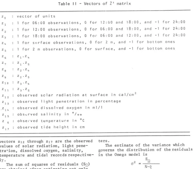
Table I I - Vectors of Z' matrix
Z o
. Z 1
Z 2
Z 3 Z"
Z 5
veetor for for for for for
Z6 Zl'Z"
Z7 Zl'zS
ze z2'z"
Z9 Z2' Z S
ZlO Z3'Z"
Zll Z3'ZS
of units
06:00 observations, G for 12: O O and 18: O O ,
12: O O observations, O for 06:00 and 18: O O,
18: O O observations, O f o I" 06:00 and 12: O O,
surfaee observations, O for 2 m, and - 1 for
2 m observations, O for surfaee, and - 1 for
Z12 observed selar radiation at surfaee in eal/em2
Z13 observed I ight penetration in pereentage
. Z 1 " o b 5 e r v e d d isso I v e d o x Y 9 e n i n m I / I
zlS obs"rved salinity in % 0
Z 6 observed temperature in
°c
Z17 observed tide height in em
ters.
and - 1 for 24:00
and - 1 for 24:00
and - 1 for 24:00
bottom ones bottom ones
vectors Z12 through Z17 are the observed
va1ues of solar radiation, 1ight
pene-tra~ion, disso1ved oxygen, sa1inity,
temperatu~e and tida1
recordsrespective-1y.
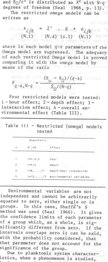
The estimate of the variance which governs the dis tribution of the residuaIs in the Omega mode1 is
The sum of squares of residuaIs (S~)
parame-and ~nYa2 is di 'stributed _; ~s ,~ i' ~th ' ~-q '
degr~és of rreedom (Sea1 ' 196'6,. ~ p~ 13) .""
The restricted omega rodet8 ' cai{ be ' written as
X.<.j
k.
(N.1)
" '0
Z' ;
o'C,-lê
'--'o+-e.;[jkt - q , : '(N~:6r )· (.ó · ~
1) ! rN:'p - ,;:, "
wheri:! in: "each mode ~ 'l ,q · :..r ~ , pàf'a~ters ) of ,the Omega 'mode! ,are sup'ressed': ' The ad~q'uácy
of ea6h 'rest'rÍ'{:!ted ' biriégarode1 ,is provEM comparirig it with the omeg? model "by
meahs of the r 'atio ' ,
'" (S .... S ' }/(q-.ó)
p
,
__
-=, w=---=n~ ,-.:. " ...,.,, ,""", __
q-.ó, N:q
$'n/
(N-q)) , '
Four restricted mode1s were tested: 1 - hour effect; 2 - depth effect;
3-interaction effect; 4 - overa11
en-vironmenta1 effect (Tab1e 111).
Table III - Restricted (omega) 'models tested
Hypothesis
w B' i -o E ff ec t
i-l,2.3 hour
i-4,5 depth
j.6, .. . • 11 depth-hour interaction
i-12, . . . ,17 environmental variables
Environmenta1 variab1es are not independent and cannot be arbitrari1y equated to zero, either sing1e or in groups. In this case, Sheffé's S
method was used (Sea1 1966). It gives the confidence 1imits of each parameter of a group which, as a who1e, is sig-nificant1y different from zero. , r . .
l i
the • interva1s overlaps zero it can be sa1d, wi th the propabi,li ty, considered" thatthat parame,ter doe$ notaccoul}t for , the
signific,ance of th,e ,group. , .
Due to planktonic system character-is tics, when a 'phenomenon 'i ,s s tudied, it is expected to find both, strong variations in 1itt1e time and space sca1es and 10ng term tendencies. In the particular case of this study space was fixed, and the expected time variations are differences of the vertical distri-bution pattern during one day in the different months; a previous study of this type, based on part of the material used in this paper, has a1ready been done
(Mi1stein, in press). More general
tendencies cou1d , be ; st,tfdi~d . -j oi~fpg :: tJiér ' data of each seasou 'or ofa!l the year. In this pap~r an : i~te~m~di :ate approach was chosen, which e1iminates part of . that variation and s'hows the tendencies in re1ative short 'periods: 2 months. In the repeti tion of the process uSirig sever-a1 groups of two monthscan .be examin~d
the variation of that tendency through.out the year. The process was reiterated nine times for each s tage of
P.
CJui6.6i.Ao.ó-:tJrJ...6, wi th the following groups orIoonths: June-Ju1y (JJ), Ju1y.:-Augus t (JA) , , Augus.t-September (AS), Novemb~r-Dec~I1l1J~~ , (~~) , J. , .
December-Janua,ry (Dl), January-February ,
(JF) , Februar~~March (FM), ~rc~:"Ap , ~i'J: :.' , ':
(MA), and Apn1-May (AM). , }hth1n each .
group envi ronmen ta1 . ~OIl<~i tions, ~e~e '
al}\<:é.
There was a gap of seven weelcs .betwee!;l .. September and November s ' ta~ions ' , and '::': general conditions (esp.ec;i.a1.1y s'âlini:ty? were so different that' the .aria1y,sis ' O'f' ,'~the group was neg1~cted. , ,'" ' ,,' , , , ':~: ~
Possible errpr. sources , '"
There are re1ative1y few , zoop1:ankton ; ;," works in which samp1e bottle weré used-.. .·J Hodgkiss (1977) made. simu1taneóus" col!"I';" 1ections with Nakai ilets atld f1: i ,·;;, "
Friedinger bottle, finding good corre.-!' r
lation between them· in :re1ation , t{) , ;; , "
seasona1 patterns of: p1-ankt0.n-io., pOpU'1"" ~, J ! :. 1ation distributions, but litt1e. sig- · nificant corre1ations appeared in the study of vertical distribu·tions' and rel~,",
tive a:bundance of each species. , Morking' wi th 2 i vanDom bottles, Stickney ,& , ;" Know1es (1975) found : that P.óe.(Ldo:dú;tp-tÇJ,'
mU6 c.aMna;tw." Ne.amlf-6.i.6 ameJÚc.ana, ad~.ü ts, of Ac.aJltia -ton.6a and other copepods , oJ + similar si'ze , ; were , negatively sele.cte;q; ,," at the same time, Elrte.np-tl1a tlç,uti.ónonó ..;·.
and other smallorganisms were s~tably; !
represented in the ,samples. Tun :disi ~ <, ':-:'. (1972,), in spi te ·of working wi th ,;l big~er samp1e bott1e (8i modifie,d Petberson- i ,
Nansen) a1so fo'und that. the adu1 ts o,f the ; bigger species we're negati vely sel~ : cted ',,';
(Ac.aJt.:ti:.a ~ j eboJtgi, P -6'e.udocUap-tomU;6 ,·, '1 ac.utu.6, Labidoc.e.Jta 6iuvi~) and the
sma11er copepods adequate1y samp1ed
(P.
70
Table IV
-
Percentage ofP.
C!l.M6ÚW6-tJrM, in surface net and
bottle samp I es
June, 06:00 March , 12: o o March, 24:00
net bottle net bot t I e net bot t 1 e
Females 42.9 46. 1 42.6 33 . 3 65 . 9 66.6 Males 40 .3 44.7 22.3 15.9 17 . 3 17.3
C.V males 4.6 O .6 11 . O 12. O 7.6 6.4
C. V females 5.3 5.3 11 . 5 17 . 7 5.1 4 . 7
C. IV 6.S 3.4 12.7 21 . 1 4 . O 5 . O
size net; they were still less repre-sented in samples of surface net (75 micra mesh size).
PaJtac.a1.a.nU6
qua..õ.únodo,
which is biggerthan
P.
C!l.M-6,ttW-6:tJvL6 but very similar to it, has been frequently found in the samples. The nauplia of the two species can be told one from the other only by their size and the diameter of metasome. In some samples appeared PaJtac.atanu-6nauplia I and 11, which still have no metasome developed; they were not counted because it was not possible to know to which of the two species they belonged.
Nauplia 111 to VI were counted sepa-rately, but were considered as a group in the statistical analysis, because there were many samples wi th few of these organisms.
The following requirements of least squares technique are fulfilled
(Hoffmann & Vieira, 1977): a - fixed
values of independent variables chosen a pr~or~; b - independent variables free of error; the small variations in depth of sample bottle or in the hour of beginning and end of sampling s tation
that could happen can be disregarded and the two variables considered free of error; c - due to the left skewed frequency distribution of the numbers of animaIs in the samples the loga-rithmic transformation used aims to make i t more normal; because of this more normal distribution the distribution of the residuaIs are assumed to be
N(0,a
2 );d - the logarithmic transformation also stabilizes the variance, and it was assumed that the residuaIs were homocedastic.
Nauplia analysis of JJ was not per-formed due to the accidental lost of alI of them of the surface 24:00 hours sample.
Four to six covariables were con-sidered in each analysis, due to 1ack of light penetration percentages in
Sep-Bolm Inst. oceanogr., S Paulo, 28(2), 1979
tember, solar radiation data in February and March, and tida1 records in December, April and May.
Results
X2 tests of goodness of fit of the 89
Omega models were computed (Tab1e V). It was a1so made a X2 test of those 89
X
2 , which showed that the fit wassui-table (1.209 for 3 df) at 0.05 signifi-cance leveI. The non significant ;0.05 X2 shown in Tab1e Vare due to random
variability; they are those expected to
JJ JA AS NO OJ JF FM MA AM
JJ JA AS NO OJ JF FM MA AM
Table V - X2 values of the 89 OMEGA
models.
**:
0.01signifi-cance leveI; df: degrees of freedom
df 6emafe6 mafe6 C. V mafe~ C. V 6 em. C. I V
0.22" O. 19" 0 . 59" 0 . 09" O . 16" 0.22" 0.S4" 0.63" 0 . 14" 1 . 1 3' 0.36" 0.S3" O . SI " 0.44" 0.66" 0.06" 0.21" 1. 96' 0.50" 0 . 79" 0.12" 0 . 59" 1. 41 ' 1.13" 0.96" 0.47" 1 .53' 0.53" O. SI" 0 . 47" 1.23' 1 . 05" 1. 51' 1 . 62' 2 . 29 0. 47" 1. 03" 1 . 33" 2.0S' 2. OS'
0.S2" 4.51 4.06 3. 2 5 2 . SS
C. III C. II C. I Copepod. Naupf.i.a
0 . 46" 1 . 02' 1 . S 3 O. 17"
6 O . 97' 0 . 62" 0 . 69" O.oS" O.6Ó" 0.23" O .65" 0.69" 0.005" C.' 64"
1. 11 " 1. 22" 0.93" 0.039" 0 . 66"
2.0S' 0.70" 0 . 2S" 0 . 032" 0.82"
1. 39' 0.25** 0.28" 0.031" 0.49" 2.00' 0.93" 0.62" 0 . 002" 0 . 79" 3.5S 2 . 3S' 1 . 52" 0.02" 0 . 75" 3.73 3.S7 2.44 0.004" 0.37"
happen with a probabi1ity of 5% if the Omega models show goodness of fit with a probability of 95%. The fact that most of these no significant records occurred in AM has probably some relation to a phytoplankton bloom which took place in May; only few zooplankters were present
in May's samp1es.
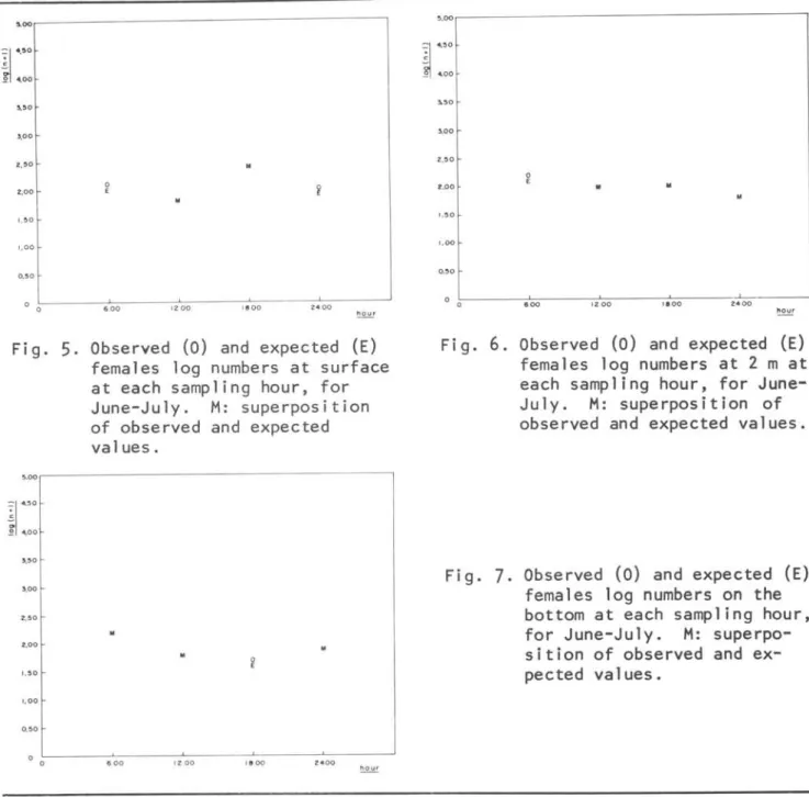
As an examp1e, it was chosen one omega mode1 to p10t observed and expected values. Figures 5, 6 and 7 show, for each depth, observed mean (O) of June and Ju1y females log (n+1) numbers at the four sampling hours, and the expected values (E) predicted by the Omega model corre-sponding to those months.
Results of comparisons between each restricted (Omega) mode1 to the general
0.00
il :::
"003,00
2,'0 M
2,00
I.~O
1, 00
0,50
6 .00 1200 1800 2400
Fig.
5.
Observed (o) and expected (E)females 10g numbers at surface at each sampling hour, for June-July. M: superposition of observed and expected values.
0.00,.-- - - -- - - ,
i1
4 '00
~ 4,00
3,00
2,50
2,00
1,00
.00 1200 I fi 00 2400
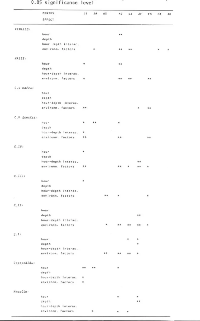
separately for each developmental stage (0.05 and 0.01 significance leveIs).
At first glance at Table VI, it can be seen that the amount of P. ~~~
~~~ of any developmental stage is
diversely affected by the different factors throughout the year, and that these effects are stronger in summer.
The hour was not always significant for any developmental stage. Mbst significances occurred in ND, in adul ts, C. V female, copepodids (as a group) and nauplia. Nauplia and C. I also showed significance in other summer months-groups, and C. 111, C. IV, C. V
females, copepodids joined and males in winter. The hour at which the greatest abundance was recorded was generally the same in the same couple of months for alI developmental stages, and
different in different couples of months.
71
0.oo,.--- - - -- - - --,
~ 4.00
~ 4,00
3.00
2,00
1,00
~---7 •. oo~--~1~20=0--~I .~0 70--~Z~----~
Fig.
6.
Observed (O) and expected (E) females 10g numbers at 2 m at each sampling hour, for June-July. M: superposition of observed and expected values.Fig.
7.
Observed (O) and expected (E) females 10g numbers on the bottom at each sampling hour, for June-July. M: superpo-sition of observed and ex-pected values.This suggests that the amount of organisms at a given hour depends more on the currents (tides) than on animaIs be-haviour in relation to hour.
Depth was significant only for C. I, C. II and nauplia in JF, which in that moment were on the bottom. This suggests that animaIs are generally spread in the water column.
Depth-hour interactions showed sig-nificance also in few occasions, pointing out that none of the developmental stages of P. ~~iha~~ performs regular
vertical migration.
Overall environmental effects were significant many times in alI stages
(except in copepodids grouped), es-pecially in ·summer; in winter they were not significant for C. I, C. 11 and C. 111.
confi-72 Bolm Inst. oceanogr., S Paulo, "28(2),1979
Table VI Results of the compar i sons between the restricted models
and the
OMEGA
rrode I .**:
0.01 significance I eve I ;*:
0.05 significance leveI
IIONTHS JJ JA AS NO OJ JF FII MA Ali
EFFECT
FEMALES :
hour **
depth
hour ~ep t h interac.
environm . factors * ** ** *
MALES:
hour * **
depth
hour-depth interac.
envlronm. factors * *.
••
••
C.V male~:
hour depth
hour-depth interac.
environm. factors
••
•
**C.V 6emale~:
hour * *. *
depth
hour-depth interac. *
environrn . factors ** ** **
C.IV :
hour *
depth
hour-depth interac. **
environm. factor. ** ** * ** *
C. II I:
hour
•
depth
hour-depth interac.
env i ronm. factors ** * *
C. II :
hou r
dept h .*
hour-depth interac.
environm. factor. * ** ** ** *
C. I :
hour * *
depth *
hour-depth interac .
env i ronm . factors ** *. *. *
Copepod-i.d~:
hour • * * • *
depth
hour-depth interac . * envi ronm. factors *
Naupl-i.a:
hou r • *
depth **
hour-depth interac.
dence limits found through Sheffé's method for the parameters which measure
their effect were tibsurdly wide, due to the small number of observations (24) in each analysis (Seal 1966, p. 62).
Discussion
Zooplankton vertical migration are tra-ditionally studied plotting amount or percentage of animals as a function of depth and hour of sampling. In both cases, interpretation is easy when there are many organisms and vertical distri-bution pattern changes clearly wi th time. Perccntages can lead to wrong conclusions, especially when few zooplankters are present.
Several authors made use of more ob-jective methods. Moore (1953) developed a method to study the vertical distri-bution of species in relation to the depth in which a certain percentage of
the population is found, and not to the absolute depth; this method was improved and completed through the study of vari-ations throughout the day of physical factors effects on animal's distribution (Moore
et all,
1953; Moore, 1955; Moore&
Corwin, 1956; Moore&
O'Berry, 1957;Moore
&
Bauer, 1960). Vinogradov (1970) developed another method to measure vertical migration intensity; these two methods need continuously sampled water layers (net samples). Angel&
Fasham (1973) introduced factor analysis in the study of vertical migration as a way of grouping species of similar vertical migration behaviour; this analysis was used later by Angel&
Fasham (1974) and Marlowe&
Miller (1975). The analysis of variance was used in the s tudy of day-night plankton sample variability (Glover&
Pope, 1956; Sameoto, 1975), and inthe study of vertical migration proper (Pearcy
et all,
1977).In the present paper the statistical method utilized includs an analysis of variance, with the advantage that the sums of squares of residuals are obtained estimating not only the mean, but other 15 or 17 parameters as well, and that the multiple regression on the environ-mental variables are computed in the same model; this is the first time that this model is fitted to this kind of data.
Differences in vertical migration behaviour of different developmental stage.:.i and sexes of holoplankters have been pointed out in classical papers
Russe1, 1927; Cushing, 1951) and in
73
modern reviews (Banse, 1964; Vinogradov, 1970; Longhurst, 1976). In spite of that, most of vertical migration re-searchers still work at the species level and do not state clearly which stages were studied. Bradford (1970) draws attention on this problem, and studies separately the vertical migration of males and females of each species in her material.
In shallow waters there were found both, copepods which do present different vertical migration behaviour in their different stages and copepods which do not show these differences. In samples
collected at short intervals throughout one day, Furuhashi (1976) found a greater difference between day and night numbers
of A~antia
ctaUói
males at surface thanof females, and some little differences between both sexes of Pana~alanUó sp and
OLthona nana.
Working wi th materialcol-lected with the same kind of sample program, Grindley (1977) found that peaks of abundance of several developmental stages of A~antia
fongipatelta
occurred at the same hour but the percentage of migrating adults were greater than that of copepodids; no difference was foundin P~eudodiaptomUó h~~ei; the author
does not give data separately for each stage of P. CACt6~Á.JtMtJú.6. Bjornberg & Wilbur (1968) contrasted the vertical migration of adult A~~a ~jebo~gi
and the lack of this phenomenon in their copepodids. Conover (1956) marked the same fact for
A.
ctaUói
and A. to~a.
Differences in
P.
~~Á.Jto~~ males and females behaviour were alreadypointed out in a previous paper (Milstein, in press) based on noon and midnight samples of the saroe material studied here. In that pape r was stated that both sexes were spread in the water
column but that males showed a weak tendency to concentrate near the bottom, especially at noon; correlation coef-ficients of numbers of males (or their logarithms) to depth were low (1ess than 0.35); correlation coefficients of
74
second case the results rose from an analysis of variance of four hours data of eleven two-month groups. The compu-tation of alI the data of alI the year by means of the Omeg.? model could confirm or nullify the weak tendencies found through the simple correlation analysis.
Bjornberg
&
Wilbur (1968) studiedP.
~~~o~~' vertical migration in the
laboratory; animaIs were generally spread in the water column, showing a weak vertical migration cycle: they concen-trate in the surface at night and on the bottom during lighthours. Grindley
(1977), worktng with samples collected at short intervals throughout one day, noticed that
P.
~~~o~~ was present at surface alI the day, but in greater numbers during darkhours.In the first work on Ubatuba's ma-terial (Milstein,
op . .
:.,i;t) it was foundthat when these animaIs showed vertical migration they were very weak and of the
inverted type in summer (during daylight in the surface layer and at night on the bottom). In the present paper a proba-bilistic model was used, which is gener-ally more objective and reliable than a graphical analysis, especially when the graphics only show tendencies and not clear behaviours; besides, the log transformation used tends to minimize weak behaviours. These two consider-ations explain the discrepances between
the results of the present paper and those of the already mentioned articles by Bjornberg
&
Wilbur, Grindley and Milstein; the differences in the amount of animaIs collected in the various depth-hour combinations are those expected to be found with 95% probability if these organisms do not migrate strongly. Clear migrations became evident only three times in 89 analysis, which suggests the lack of a clearly developped migra-tory behaviour in alI the developmental stages ofP.
~~~o~~ throughoutthe year.
The influence of environmental factors on vertical distribution of
P.
~~~~o~~ became evident in most analysis
of the present paper. It was not possi-ble to study each factor alone. In the previous paper (Milstein,
op. W.)
simplecorrelation coefficients between numbers of adults (absolute and log numbers) and salinity, temperature and dissolved oxy-gen were calculated, and tidal effect on the variation of P. cJtM~~M~~
a-bundance was discussed. Females proved to be more euroic than males, showing only low corre1ation to temperature;
Bolm Inst. oceanogr., S Paulo, 28(2), 19J9
males showed corre1ation to sa1ini ty on1y at midnight, and stronger corre1ation to temperature at noon and at midnight; no corre1ation to dissol ved oxygen was found. Lance (1964) studied sa1inity to1erance of severa1 estuarine crus-taceans, and found that fema1es were IIDre to1erant t :lan males and copepodids. It is evident the significance of environ-mental factors on zooplankton distri-bution, and the different responses of fema1es, males and young forms to them; these factors proved to be more important
for P. ~~~o~~ than depth and hour.
In connection to tides, in the previous paper (Mi1stein,
op.cit)
more organisms were recorded at high tide. Jacobs (1968) and Pi11ai&
Pi11ai (1973) a1so found more animaIs at high tide, and a combination of tida1 and vertical migration effects on the distribution of organisms. Grind1ey (1977) a1so found a superposition of tidal effect and verti-cal migration: at night the numbers ofP.
cJtM~~O~~ and other plankterswere lower at low tide than the rest of the night; during the day there was no difference between their numbers at low and high tides. Sameoto (1975) found tidal corre1ation to numbers of severa1 nonmigrating copepods; migrating anima1s did not show tida1 correlation. In a general way it could be said that, in shal10w waters, animal concentration are greater at flood than at ebb, and that this effect is stronger in organisms that show weak vertical rrigration than in p1ankters that can partially "escape" to it through their migratory behaviour.
P.
~~~~~ be10ngs to the firstgroup; in the present paper it seems that hour was signifícant due more to tidal effect than to itself, because those significant points appeared only few times for each stage and a1most always in the same groups of months for several stages (JJ and NO) .
Bjornberg
&
Wilbur(op.cit)
re1ated vertical migration of copepcds to feeding behaviour: strong vertical mi Gration in predators and weak ones in fine partic1e grazers; in shallow waters there are fine particles suspended at a11 depths, and grazers of these partic1es showed weak vertical migration(P.
~~ÁÁfl~~ andAQahtia
~jebong~ copepodids);zoo-p1ankton accumu1ates on the bottom during daylight in sha1low w~ters, and
predators (Calanop~a am~Qana) showed
MILSTEIN:
PanaQa!anU4
~~~O~~correlation coefficier. ':s among alI plank-tonic species in his samples, and could tell a vertical migrating community of predators from a nonmigrating community of preys consisting of copepods. The re-sults of the present paper support these ideas, showing the lack of vertical mi-gration in alI stages of a coas tal water copepod which is a fine particle grazer during alI its life.
As it was pointed out in the statistical analysis section this linear model can be fitted to the data of several clustered months in order to study more general tendencies; that stuJy, based on the same data of this paper, will be
de-velop~d in future research.
Ackno~Jl edgements
I would like to thank Dra. Maria Scintila
de Almeida Prado for her help and guidance throughout this study, and to the "Ins-tituto Oceanográfico da Universidade de são Paulo" for allowing me the use of
the facilities of the Department of Biological Oceanography and of the coas tal station at Ubatuba.
Resumo
A distribuição vertical dos diferentes estádios de desenvolvimento de
P.
Q~ ~~O~~ foi estudada durante um ano
(junho 1976 - maio 1977), numa estação pouco profunda (5 m) em Ubatuba. As amostras foram coletadas mensalmente, em três profundidades, cada quatro ho-ras, com garrafa van Dorn de 9 l, re-gistrando-se dados ambientais.
Os dados foram processados com a tecnica dos Mínimos Quadrados, na for-ma de ufor-ma Ar-álise de Regressão de um Modelo Linear que inclui covariáveis. O modelo foi construído a priori,
con-siderando densidade de organismos por amostra, fatores ambientais, diferenças entre amostras procede~ ' tes de
diferen-tes profundidades e horas, também como interações entre hora e profundidade. Para cada estádio de P. cAaM~o~ 7tM, o modelo foi repetido 9 vezes, com os dados de dois meses cada vez, a fim de obter a variação das respostas no ano.
Os resultados do modelo indicaram que a quantidade de indivíduos desta especie de qualq "er estádio é diferen-temente afetada durante o ano pela ho-ra, profundidade, interação hora-pro-fundidade, e fatores ambientais. Es-ses efeitos seriam mais marcados no ve-rão. A maior ou menor ocorrência de
75
organismos numa dada hora parece depen-der mais da dinâmica do sistema de cor-rentes (marés) que do comportamento dos animais. Todos os estádios apresenta-ram-se distribuídos na coluna de água e não mostraram migrações vertica;s mar-cadas como parte do seu comportamento normal. Os fatores ambientais em con-junto mostraram-se importantes na dis-tribuição_deste organismo, especialmen-te no verao.
Bjornberg
&
Wilbur (1968) e Sameoto (1975) relacionaram o comportamento mi-grador pouco marcado ou ausente com o nível trófico que os planctontes cos-teiros ocupam. Os primeiros autoresas-sinalarG~ a presença de partículas finas
em todas as profundidades em águas rasas, e a migração pouco definida de copépodos filtradores provenientes desse tipo de á-gua; o segundo autor distinguiu, em águas pouco p~")fundas também, uma comunidade formada por predadores e uma comunidade de p .. :esas formada por copepodos não mi-gradores. Os resultados do presente tra-balho apóiam essas idéias, mostrando a
falta de migração em todos os estádios de um copépodo que é, durante toda a sua
V1-da, filtrador de partículas finas.
B i b 1 i og r a ph y
AMARAL, A. C. Z. 1977. Anelídeos poli-quetos do infralitoral em duas enseadas da região de Ubatuba: aspectos ecoló-gicos. Tese de Doutorado. Universi-dade de são Paulo, Instituto Oceano-gráfico, 140 p.
ANGEL, M. V.
&
FASHAM, M. J. R. 1973. SOND cruise~ 1965: factor and clusteranalyses of the plankton results, a general summary. J. mar. biol. Ass. U. K., 53:189-231.
1974. SOND cruise, 1965: further factor analyses of the plankton data. J. mar. biol. Ass. U. K., 54:879-894. ANRAKU, M. 1964. Influence of the Cape
Cod Canal on the hydrography and on the copepods in Buzzards Bay and Cape Cod Bay, Massachusetts. I. Hydrography and dis tribution of copepods. Limnol. Oceanogr., 9(1):46-60.
BANSE, K. 1964. On the vertical distribution of zooplankton in the sea. Progr. Oceanogr., 2:53-125. BARNES, H. 1952. The use of
sta-76
tistics. J. Cons. perm. int. Exp1or. Mer, 18:61-71.
BJORNBERG, T. K. S. 1963. On the marine free-1iving copepods off Brazi1. Bo1m Inst. oceanogr., S Paulo, 13(1): 3-142.
1972. Deve10pmenta1 stages of some tropical and subtropi-cal p1anktonic marine copepods . Stud. Fauna Curaçao, 40(136):1-185.
& WILBUR, K. M.
1968. Copepod phototaxis and vertical migration influenced by Xanthene dyes. Bio1. Bu11. mar. bio1. Lab. Woods Ho1e, 134(3):398-410.
BRADFORD, J. M. 1970. Diurna1 vari-ation in vertical distribution of pe1agic copepods off Kaikoura, New Zea1and. N.Z.J1.mar. Freshwat. Res., 4(4) :337-350.
BUZAS, M. A. 1969. Foraminifera1 species densities and environmenta1 variab1es in an estuary. Limno1. Oceanogr .. , 14:411-422.
1971. Ana1yses of species densities by the mu1tivariate general linear mode1. Limno1. Oceanogr., 16: 667-670.
CONOVER, R. J. 1956. Oceanography of Long Is1and Sound, 1952-1954. VI .. Bio10gy of Ac.o.JI.;tia.
ua.uói
andA.
tOV1.J.>a.Bu11. Bingham oceanogr. Co11., 15:156-233.
CUSHING, D. H. 1951. The vertical migration of p1anktonic CLustaceans. Bio1. Rev., 26(2):158-192.
DARO, M. H. 1974. ~tude des migrations nyctemera1es du zoop1ancton dans un mi1ieu marin peu profond. Hydro-biologia, 44(2-3):149-160.
DEVASUNDARAM, M. P. & ROY, J. C. 1954. A preliminary study of the p1ankton of the Chi1ka Lake for the years 1950 & 1951. FAO/UNESCO, Symp. Mar. Freshw. P1ankton in the Indo-Pacific, Bangkok, p. 48-54.
DIXON, W. J., ed. 1974. Biomedica1 computer programs. Berke1ey, Univ. California Press, 773 p.
ENRIGHT, J. T.
&
HAMMER, W. M. 1967. Vertical migrations and endogenous rhythmicity. Science, N. Y., 157(3791) :937-941.FERNANDEZ, F. da C. 1977. Contribuição
ã ecoloeia dos bivalves do
infrali-Bolm Inst. oceanogr., S Paulo, 28(2),1979
tora1 de fundos moles da região_de Ubatuba (são Paulo). Dissertaçao de mestrado. Universidade de são Paulo, Instituto Oceanográfico, 70 p.
FURUHASHI, K. 1976. Die1 vertical mi-gration suspected in some copepods and chaetognaths in the in1et waters, with a specia1 reference to behavioura1 differences between ma1e and fema1e, noted in the former. Publs Seto mar. bio1. Lab., 22(6) :355-370.
GLOVER; R. S.
&
POPE, J. A. 1956. The Hardy p1ankton indicator: a study of the variation between catches taken . by day and by night. Bull. l'lar. Eco1., 4(32) :115-134.GRICE, G. D. 1960. Calanoid and cyc1o-poid copepods co1lected from the Florida Gu1f Coast and Florida Keys in 1954 and 1955. Bul1. mar. Sci. Gu1f Caribb., 10(2):217-226.
GRINDLEY, J. R. 1972. The vertical migration behaviour of estuarine p1ankton. Zool. afr., 7(1) :13-20.
1977. The zooplankton of Langebaan Lagoon and Sandanha Bay. Trans. R. Soc. S. Afr., 42(3-4):341-370.
GURNEY, R. 1927. Copepoda and Cladocera of the p1ankton. Trans. zool. SOCo Lond., 22:139-172.
HODGKISS ,
r.
J. 1977. The useofsimu1-taneous samp1ing bott1e and vertical net co11ections to describe the dy-namics of a zoop1ankton population. Hydrobio1ogia, 52(2-3) :197-205.HOFFMANN, R.
&
VIEIRA, S. 1977. Análi-se de regressão, uma introduçaõ ã Eco-nometria. são Paulo, HUCITEC/EDUSP, 339 p.JACOBS, J. 1968. Animal behaviour and water movement as co-determinants of
p1ankton distribution in a tidal system. Sarsia, 34:355-370.
JlMENEZ, A., M. P. 1976. Distribuição vertical e estádios de
desenvolvimen-to de Luc.i6~
6axoni
Borradaile (Crustacea) ao largo de Santos. Dis-sertação de mestrado. Universidade de são Paulo, Instituto de Biociências,54p. .
LANCE, J. 1962. Effects of water of reduced sa1inity on the vertical migration of zoop1ankton. J. mar. biol. Ass. U. K., 42:131-154.
of some estuarine planktonic crus-taceans. Biol. Bull. mar. biol. Lab. Woods Hole, 127(1):108-118.
LAWSON, T. L.
&
GRICE, G. D. 1973. The developmental stages of P~acalanU6~a6~~O~~ Dahl, 1894 (Copepoda;
Calanoidea). Crustaceana, 24:43-56. LEWIS, A. G. 1959. The vertical
distri-bution of some inshore copepods in relation to experimentally produced conditions of light and temperature. Bull. mar. Sei. Gulf Caribb.,
9:69-78.
LONGHURST, A. R. 1976. Vertical mi-gration. In: Cushing, D. H. &
Walsh, J. J., eds. - The ecology of the seas. Oxford, Blackwell, p.
116-137.
MARLOWE, C. F.
&
MILLER, C. B. 1975. Patterns of vertical distribution of. "p"
zooplankton at ocean stat10n . Limnol. Oc.eanogr., 20(5):824-844. MILSTEIN, A.,
PaJta.c.a.tanU6
~a6~~O~~ (Copepoda: Calanoidea):
variations of its abundance in a shallow water station. Anais Acad. bras. Ciênc., Supl. (no prelo)
MOORE, H.B. 1933. Plankton of the Florida Cur=ent. 11. Siphonophora. Bull. mar. Sei. Gulf Caribb., 2(4): 559-573.
1955. Variations in
temperature and light response within a plankton population. Biol. Bull. mar. biol. Lab. Woods Hole, J08(2): 175-181.
& BAJER, J. C. 1960. An
analysis of the relation of the vertic, distribution of three cope-pods to _nvironmental conditions. Bull. mar. Sei. Gulf Caribb., 10(4): 430-443.
&
COR~IN, E. G. 1956. Theeffects of temperature, illumination and pressure on the vertical distri-bution of zoop'.ankton. Bull. mar. Sei. Gulf Caribb., 6(4)~273-287.
&
O'BERRY, D. F. 1957.Plankton of the Florida Current. IV. Factors influencing the vertical distribution of some common copepods. Bull. mar. Sei. Gulf Caribb., 7 (4): 287-315.
OWRE, H.; JONES, E. & DOW, T. 1953. Plankton of the Florida Current. 111. The control of the
vertical dis tribution of the zoo-plankton in the daytime by light and temperature. Bull. mar. Sei. Gulf Caribb., 3(2):83- 95.
77
MOREIRA, M. G. S. 1973. On the diurnal vertical' migration of Hydromedusae off Santos, Brazil. Publs seto mar. biol. Lab., 20:537-566.
1976. Sobre a migra-ção vertical diária do plâncEon ao largo de Santos , Estado de Sao Paulo, Brasil. Bolm Inst. oceanogr., S Paulo, 25(1):55-76.
PEARCY, W. G.; KRYGIER, E. E.; MESECAR,
R. & RAMSEY, F. 1977. Vertical
distribution and migration of oceanic micronekton off Or egon. Deep-sea Res., 24(3):223-246.
PILLAI, P. P. & PILLAI, M. A. 1973. Tidal influence on the diel variation of zooplankton with special refer-ence to copepods in the Cochin Back-water. J. mar. biol. Ass. India,
15(1) :411-417.
PIRES, A. M. S. 1977. Aspectos ecoló-gicos da fauna de Isopoda (Crustacea: Peracarida) das zonas litoral e in-fralitoral de fundos duros da Ensea-da do Flamengo, Ubatuba, são Paulo. Tese de Doutorado. Universidade de são Paulo, Instituto Oceanográfico, 83 p.
ROCHA, C. E. F. da 1977. Distribuição dos Cladocera e Ostracoda (Crustacea) planctônicos marinhos ao largo de Santos, Brasil. Dissertação de
Mes-trado. Universidade de são Paulo, Instituto de Bi ociências, 100 p. RUDYAKOV, Yu. A. 1971. Details of
the horizontal distribution and di-urnal vertical migrations of Cyp~
~na (PyhOC.yp~) ~~nuo~a (G. W.
Müller)(Crustacea, Ostracoda) in the western equatorial Pacifico In:
vi-nogradov, M. E., ed. - Life activi-ty of pelagic communities in the ocean tropics. Jerusalem, Israel Program for Scientific Translations,
p. 240-255.
RUSSELL, F. S., 1927. The vertical distribution of plankton in the sea. Biol. Rev., 2:213-262.
environ-78
ment. J. Fish. Res. Bd Can., 32(3): 347-366.
SCHAEFFER-NOVELLI, Y. 1976. Alguns as-pectos ecológicos e análise da popu-lacão de
Anornaloeandia
b~~ana(G~~:in, 1791) Mollusca, Bivalvia, n~
praia do Saco da Ribeira, Ubatuba, Estado de são Paulo. Tese de
Douto-rado. Uniyersidade de são Paulo,
Inst~tuto de Biociências, 118 p.
SEAL, H. L. 1966. 'Multivariate sta-tistical analysis for biologists. London, Methuen, ~07 p.
SEWELL, R. B. S. 1948. The free-swimming planktonic Copepoda. Geograp~1Ícal
distributicn. Scient. Rep. John Murray Exp., 8(3):317-592.
STICKNEY, R. R.
&
KNOWLES, S. C. :975. Summer zooplankton d;stribution in a Georgia estu~ry. Mar. Biol., 33(2):147-157.
Bolm Inst. 0ceanogr.,
S
Paulo,28(2),1979
TEIXFlRA, C. 1973. Prclimin<lr} s tudies
of pri~ary production in the Ubatuba
region(Lat. 23°30'S - Long. 45°06'W), Brazil. Bolm Inst. oceanogr., S Paulo, 22:49-58.
---; TUNDISI, J. & KUTNER, M. B. 1965. Plankton studies in a mangrove environment. 11. The standing-stock and some ecological factor3. Bolm Inst. oceanogr., S Paulo, 14(1) :13-4l.
TUNDISI, T. M. 1972. Aspectos ecológi-cos co zooplâncton da região lagunar de Cananéia com esp~cial refe~ência
aos Copepoda (Crustacea). Tese de Dout0rado. Universidade de são Paulo, Instituto de Biociências, 191 p, VINOGRADOV, M. E. 1970. Vertical
distribution of the oceanic zoo-plankton. Jerusalem, Israel Program for Scientific Transbtions, 339 p. YAMAZI, I. 1957. Plankton investigation
in inlet waters a'ong the coast of Japan. XX. Diurnal change of plankton an1mals aL an innermost station in Wakayama Harbour. Publs Seto mar. hiol. Lab., 6(2):209-224.