UNIVERSIDADE DO ALGARVE
Affine Image Registration Using Genetic
Algorithms and Evolutionary Strategies
Mosab Bazargani
Mastrado em Engenharia Inform´atica
Affine Image Registration Using Genetic
Algorithms and Evolutionary Strategies
Mosab Bazargani
Tese orientada por
Fernando Miguel Pais de Gra¸ca Lobo
Thesis submitted in conformity with the requirements
for the degree of Master of Science
Graduate Department of Computer Science
Universidade do Algarve
Abstract
This thesis investigates the application of evolutionary algorithms to align two or more 2-D images by means of image registration. The proposed search strategy is a transformation parameters-based approach involving the affine transform. A noisy ob-jective function is proposed and tested using two well-known evolutionary algorithms (EAs), the genetic algorithm (GA) as well as the evolutionary strategies (ES) that are suitable for this particular ill-posed problem. In contrast with GA, which was originally designed to work on binary representation, ES was originally developed to work in contin-uous search spaces. Surprisingly, results of the proposed real coded genetic algorithm are far superior when compared to results obtained from evolutionary strategies’ framework for the problem at hand. The real coded GA uses Simulated Binary Crossover (SBX), a parent-centric recombination operator that has shown to deliver a good performance in many optimization problems in the continuous domain. In addition, a new technique for matching points, between a warped and static images by using a randomized ordering when visiting the points during the matching procedure, is proposed. This new tech-nique makes the evaluation of the objective function somewhat noisy, but GAs and other population-based search algorithms have been shown to cope well with noisy fitness eval-uations. The results obtained from GA formulation are competitive to those obtained by the state-of-the-art classical methods in image registration, confirming the usefulness of the proposed noisy objective function and the suitability of SBX as a recombination operator for this type of problem.
Keywords: Evolutionary algorithm (EA), image registration (IR), affine trans-form, point-pattern matching, genetic algorithm (GA), evolutionary strategies (ES), sim-ulated binary crossover (SBX).
Acknowledgements
I would like to thank all those collaborators who helped me in the process that now comes to completion with this thesis.
First and foremost, I want to thank my supervisor Fernando G. Lobo. Without his support and patience, this thesis would not have been possible. I am indebted to him for his help and support, and will always appreciate the time and consideration that he devoted to my work.
Kind gratitude to my beloved family, my mother who passed away in my embrace and on her peaceful face was pictured the whole world’s love, my father and two sisters who taught me to be myself. They taught me to never give up in achieving my ultimate goals. They are the spiritual support of my life. A very special thanks goes to Houman Samim, my brother in law, who has always been there for me.
I am very thankful to Ali Mollahosseini, who I first met two years ago, and since then until he left to the USA we were working in the same laboratory. We interacted intensely on a daily basis. I would also like to thank him for all the scientific and social discussions we had.
I am also very grateful to Ant´onio dos Anjos and his family, especially his father whom I take my hat off to. Some of the ideas presented in this thesis resulted from discussions Ant´onio and I had. He always tried to encourage me to learn more and more in computer science area.
Kind gratitude to Ana Cristina Pires and Gil Guilherme, my Salsa teachers, who showed me a new path in my life. I would also like to thank all my salsa friends, for their understanding, kindness and companionship, for all the great times we shared.
How can I forget Denise Candeias for all her help at the final stage of my writing. Last but not the least, I would like to thank all my colleagues and friends, for being there always with me whenever needed.
Contents
1 Introduction 1
1.1 Motivation . . . 1
1.2 Objectives . . . 3
1.3 Contributions . . . 3
1.4 Organization of the Thesis . . . 4
2 Genetic Algorithms and Evolution Strategies 7 2.1 Introduction . . . 7
2.2 Natural Evolution . . . 8
2.3 History of Evolutionary Computation . . . 11
2.4 Evolutionary Algorithms . . . 13
2.4.1 Components of Evolutionary Algorithms . . . 14
2.4.1.1 Representation . . . 15
2.4.1.2 Selection . . . 15
2.4.1.3 Recombination . . . 16
2.4.1.4 Mutation . . . 17
2.4.1.5 Replacement (Survivor Selection) . . . 17
2.4.1.6 Termination Condition . . . 17
2.5 Genetic Algorithms . . . 18
2.5.1 Tournament Selection . . . 19 v
2.5.2.2 Gaussian Mutation . . . 21 2.6 Evolutionary Strategies . . . 21 2.6.1 Representation . . . 22 2.6.2 Parent Selection . . . 23 2.6.3 Recombination . . . 23 2.6.4 Mutation . . . 23 2.6.4.1 Polynomial Mutation . . . 24 2.6.5 Survivor Selection . . . 26 2.6.6 Self-Adaptation . . . 27 2.6.6.1 1/5 Success Rule . . . 27
2.6.6.2 Uncorrelated Mutation with One or n Step-Size(s) . . . 28
3 Image Registration 31 3.1 Introduction . . . 31 3.2 Warping . . . 33 3.2.1 Geometric Transform . . . 34 3.2.1.1 Rigid . . . 34 3.2.1.1.1 Affine Transform . . . 34 3.2.1.2 Non-Rigid . . . 36
3.3 Estimation of the Difference . . . 37
3.4 Related Work . . . 37
3.4.1 Classical Methods . . . 38
3.4.2 EC and MH methods . . . 38
4 Application of Evolutionary Algorithms to Image Registration 41 4.1 Introduction . . . 41
4.2 Representation . . . 42 4.3 Objective Function . . . 42 4.4 GA Operators . . . 46 4.4.1 GA Experimental Results . . . 47 4.5 ES Operators . . . 52 4.5.1 ES Experimental Results . . . 53 4.6 Discussion . . . 55 4.7 Summary . . . 57
5 Conclusion and Future Work 59 5.1 Conclusion . . . 59
5.2 Future Work . . . 61
Appendix A Framework of evolutionary Strategies 63 A.1 Introduction . . . 63
A.2 The ESs Representation . . . 64
A.3 The Standard (µ/ρ+, λ)–ESs Algorithm . . . . 65
A.4 Self-Adaptation . . . 68
A.4.1 1/5 Success Rule . . . 68
A.4.2 Uncorrelated Mutation with One or n Step-Size(s) . . . 68
A.4.2.1 Mutation Rate in Binary Search Space . . . 68
A.4.2.2 Mutation Rate in Integer Search Space . . . 70
A.4.2.3 Mutation Rate in Real-Valued Search Space . . . 71
A.5 Initialization . . . 72
A.6 Parent Selection . . . 74
A.7 Variation . . . 74
A.7.1 Simulated Binary Crossover (SBX) . . . 74
A.7.2 Bit-Flip Mutation . . . 74 vii
Appendix B Application Details 81 B.1 Execution of the Application . . . 81 B.2 An Example of the Input File . . . 82
Bibliography 87
List of Figures
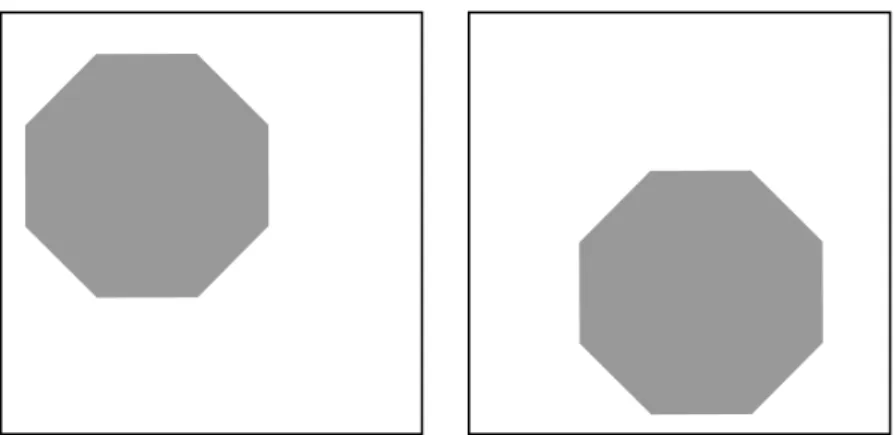
1.1 Two octagons; left: static image; right: deformed image. . . 3
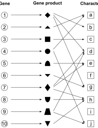
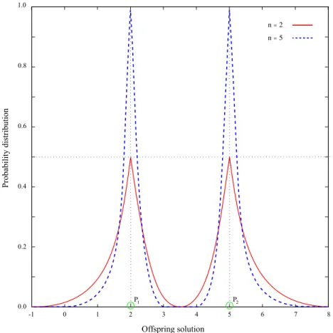
2.1 Epistatic gene interaction, and the behavior of pleiotropy and polygeny. . 10 2.2 Probability distribution, used in the simulated binary crossover (SBX),
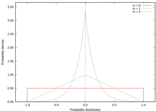
are shown for different values of the distribution index n. Figure courtesy of Deb and Jain [26]. . . 21 2.3 Probability distribution to create a mutated value for continuous variables.
Figure courtesy of Deb and Goyal [25]. . . 25
3.1 Finding a transformation by point correspondence. . . 32 3.2 Elementary geometric transforms for a planar surface element used in the
affine transform: translation, rotation, scaling, stretching, and shearing. . 35
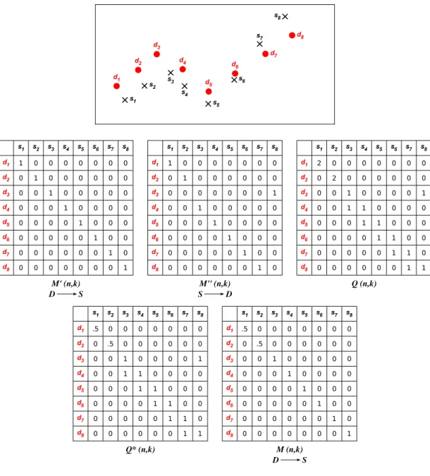
4.1 An example of the correspondence matrices: points s1, s2, s3, s4, s5, s6,
s7, s8 correspond to d1, d2, d3, d4, d5, d6, d7, d8, respectively, for mapping
point-sets D to S. However, if mapping S to D, points s1, s2, s3, s4, s5, s6,
s7, s8 correspond to d1, d2, d4, d5, d6, d7, d8, d3, respectively. . . 45
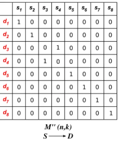
4.2 Correspondence matrix M′′(S → R): based on new match-order vector; points s8, s5, s3, s2, s1, s6, s7, s4 correspond to points d8, d5, d4, d2, d1,
d6, d7, d3. . . 46
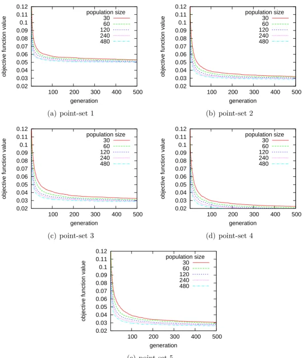
red dots are the warped image points) results obtained after 500 genera-tions using population size 120. The warped images are zoomed for better visualization. Note that even better matching could be obtained with larger population sizes, but the improvements are negligible as shown in Figure 4.4. . . 49 4.4 Best objective function value through generations for various population
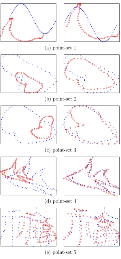
sizes obtained for various point-sets. The results are averaged over 100 independent runs. . . 50 4.5 Affine distorted point-sets and respective registration results. On the left
column, (a), the blue dots are the static image points and the red dots are the deformed image points. On the other columns, (b), (c), and (d), the red dots are the warped image points. The warped images are zoomed for better visualization. The GA results were obtained after 500 generations using population size 120. Observe that for the case of GA and TPS-RPM, the deformed and static points are almost on top of each other, meaning that the match is almost perfect. For SC the results are slightly inferior
compared with those obtained by the GA and TPS-RPM. . . 51
4.6 These images are obtained directly from [78]. The top, middle, and bottom images, correspond to our point-sets 1, 4, and 3, respectively. The blue dots are the static image points and the red dots are the warped image points. . . 52 4.7 Standard deviation of the objective function value of the population
mem-bers averaged over 100 runs with a (160 + 1120)-strategy using different mutation operators for point-sets 4 and 5. The other point-sets have sim-ilar behavior. . . 54
4.8 Best objective function value through generations for (160+1120)-strategy for various point-sets. The results are averaged over 100 independent runs. 55 4.9 Best objective function value through generations for (160+1120)-strategy
and (160, 1120)-strategy for point-sets 4 and 5. The results are averaged over 100 independent runs. . . 56 A.1 The mechanism of the transformation function (a = 6, b = 8). Figure
courtesy of Li [56]. . . 78
List of Algorithms
2.1 The general scheme of an evolutionary algorithm . . . 14
4.1 Objective function . . . 43
A.1 Outline of the (µ/ρ+, λ)–ES . . . . 67
A.2 Outline of the (µ/ρ+, λ)–ES with 1/5 success rule . . . . 69
A.3 Integer step-size mutation . . . 70
A.4 Real-valued step-size mutation . . . 71
A.5 Simulated binary crossover (SBX). . . 75
A.6 Integer object parameters mutation . . . 77
A.7 Transformation function Tr [a,b](x), for interval boundaries a and b. . . 78
A.8 Polynomial mutation. . . 79
List of Tables
4.1 Minimum square errors of affine deformed point-sets . . . 56
The aim of science is not to open the
door to infinite wisdom, but to set a
limit to infinite error.
Bertolt Brecht
Chapter 1
Introduction
1.1
Motivation
“If God had wanted to put everything into the universe from the beginning, he would have created a universe without change, without organisms and evolu-tion, and without man and man’s experience of change. But he seems to have thought that a live universe with events unexpected even by himself would be more interesting than a dead one.”
In the above mentioned quote, Karl Popper, one of the greatest philosophers of sci-ence of the 20th century, brilliantly explains the reason of the existence of evolution of
everything surrounding us. In our world today, there are problems with characteristics which are similar to the adaptation problems encountered in Nature which have been solved through evolution. Such problems occur when the task is to find the best (or a reasonably good solution) out of many possible solutions to a given problem. These kind of problems have been reported in a variety of fields such as computer science, management science, industrial engineering, biology, and many others.
Since these kind of problems are solved in Nature, it is quite rational to seek a solution for them which is inspired by Nature. Evolution provides inspiration to compute solutions
to problems that have previously appeared intractable.
All evolutionary systems process through generations, where a small change at one stage can result in large differences at a later stage. This feature is called butterfly effect. The butterfly effect is a common trope in fiction when presenting scenarios involving time travel and with hypotheses where one storyline diverges at the moment of a seemingly minor event resulting in two significantly different outcomes.
According to this theory, we would need to germinate another planet and wait several millions of years to study how life could possibly be over there after solving one problem. Since it would be impossible and also irrational we could use computer science to simulate such a world through evolutionary algorithms.
To assess how evolutionary algorithms can cope with real world problems, especially ill-posed problems, in this thesis the image registration problem is optimized by means of evolutionary algorithms.
Image registration (IR) is the process of finding the transformation that aligns one image to the other image. This is a key problem in computer vision encountered in many areas, e.g., medical image analysis, pattern recognition, face tracking, handwriting recog-nition, astro- and geophysics, and analyzing images from satellites. Image registration can be defined in a simple language with only a few words: given a static and a de-formed image, find a suitable transformation such that the transde-formed dede-formed image becomes similar to the static image. However, it is easy to state the problem but hard to solve it. The main reason comes from the fact that the problem is ill-posed. Small changes of the input images can cause completely different registration results. Further-more, the solution may not be unique. Suppose we have to register the deformed image to the static image that are depicted in Fig. 1.1. For the sake of simplicity, only rigid transformations are allowed, i.e., rotation and transformations. Several solutions can be immediately discovered, e.g., a pure translation, a rotation of 45 degrees, a rotation of 90 degrees followed by a translation, and so on.
1.2. Objectives 3
Figure 1.1: Two octagons; left: static image; right: deformed image.
In this thesis, the goal is to find the best mapping function, also called transform, that warps a Deformed image (D) in the direction of a Static image (S ), based on the images’ features (e.g. point positions).
1.2
Objectives
The thesis has the following main objectives:
• Application of evolutionary algorithms to image registration.
• Design and program a framework for evolutionary strategies in C++.
• Study a new noisy objective function using a real coded representation for image registration by means of genetic algorithm and evolutionary strategies.
1.3
Contributions
The main contributions of this thesis are:
• Propose a new technique for matching points between a warped and static im-ages by using a randomized ordering when visiting the points during the matching procedure [7].
• Application of a real coded GA to align two or more 2-D images by means of image registration. The proposed search strategy is a transformation parameters-based approach involving affine transformation. The real coded GA uses simulated binary crossover (SBX). This work has been accepted as a poster publication at ACM GECCO 2012, one of the most prestigious conferences in the EC field [7]. • Design and program a generic framework for evolutionary strategies in C++. This
framework is fully object oriented and includes the classical 1/5 success rule and the self-adaptive uncorrelated mutation strategies. Moreover, discrete, intermedi-ate, and simulated binary crossover (SBX) as recombination operators and bit-flip, geometrical, Gaussian, and polynomial as mutation operators are included. Im-plemented ingredients of the evolutionary strategies (ES) are elaborated in Ap-pendix A.
• Investigate the effect of simultaneous usage of SBX and real-valued mutation op-erators on the applications’ behavior (Sect. 5.1).
1.4
Organization of the Thesis
The thesis is composed of six chapters. Chapter 1 starts off by explaining the motivation of this work, and continues clarifying the main objectives and contributions of the thesis. It is finalized by the details of organization of the thesis.
Chapter 2 presents a brief overview of the natural evolution and the history of evolu-tionary computation. Afterwards, it introduces the evoluevolu-tionary algorithms and its key ingredients as search methods inspired by natural selection and genetics. It continues by addressing genetic algorithms and its major representations. This chapter ends by reviewing the basic procedures of standard evolutionary strategies and its terminology. Moreover, the operators used in this work are explained in this chapter.
1.4. Organization of the Thesis 5 classes, rigid and non-rigid, geometric transforms. Affine and polynomial transforms and thin plate splines (TPS) are given as examples of those classes. Additionally, some well known techniques for solving image registration problems, including both classical as well as evolutionary computation and metaheuristic based approaches are discussed.
Chapter 4 proposes a new objective function for matching points between deformed and static images by using a randomized ordering when visiting the points during the matching procedure. Then, the new objective function is studied by means of genetic algorithm and evolutionary strategies. The control parameters for both evolutionary algorithms are discussed in this chapter. It investigates the behavior of SBX in the noisy objective function. Furthermore, it discusses the behavior of evolutionary strategies and genetic algorithm for the image registration problem.
Chapter 5 concludes the thesis. Just as the thesis itself, this chapter ends suggesting some topics for future work in the application of EAs to image registration.
Chapter 2
Genetic Algorithms and Evolution
Strategies
2.1
Introduction
Evolutionary Computation (EC) covers all aspects of the simulation of evolutionary pro-cess in computer systems. It is quite a recent and tremendously growing field as well as an optimization process. The term itself was invented as recently as 1991, and represents an effort to bring together researchers who have been following different approaches to simulating various aspects of evolution [3]. Those aspects are genetic algorithms (GAs) [40, 59, 61], evolutionary strategies (ESs) [5, 12], and evolutionary programing (EP) [36, 37, 62]. Note, since last decade these aspects are extended. Although simulations of the natural evolution have been used by biologists to study adaptation in changing environments to gain insight into the evolution of the complex organisms found on Earth, it has also been shown that complex optimization problems can be solved with simulated evolution. EC techniques have been successfully applied to various optimization problems in engineering, economics, biology, chemistry, physics, and computer science.
There are many computational problems that require searching through a huge num-7
ber of possible solutions. Moreover, many computational problems require complex so-lutions that are difficult to program by hand. The classical techniques for solving com-plex optimization problems have been generally unsatisfactory when applied to nonlinear optimization problems especially those with temporal, stochastic, or chaotic elements. Nonetheless, these problems can be classified under the same group of problems that Na-ture solves itself. In other words, biological evolution is an appealing source of inspiration for computing the solutions to problems that have previously appeared intractable.
This chapter is devoted to two classes of algorithms in EC (ESs and GAs) which have been implemented and used in this work. First of all, natural evolution and history of genesis of evolutionary computation are addressed. A general scheme that forms the common basis of all evolutionary algorithms variants and its key ingredients are elaborated. Afterward, genetic algorithms are briefly described. Furthermore, it details GA operators that are applicable to representations in the continuous domain, as that will be the case for the image registration problem that is addressed in this thesis. Finally, evolutionary strategies involving self-adaptation and its components are elaborated.
2.2
Natural Evolution
In 1859, Darwin came up with the origin of species [23] which presented a theory for existence and evolution of life on Earth. According to his theory, the vast majority of the history of life can be fully accounted for by physical (evolution) processes operating on and within populations and species [48]. These processes are: replication, variation, and selection. Replication is an obvious property of extant species. In other words, it increases the population size of species that would have reproductive potential at an exponential rate if all individuals were to reproduce successfully. Variation comes about through the transfer of an individual’s genetic program (asexually or/and sexually) to progeny. Variation is introduced due to errors in the replication process, resulting in a
2.2. Natural Evolution 9 gradual development of new organisms [58]. These changes often occur due to coping errors. Sexual recombination is another form of variation and is itself a product of evolution. Competition is a consequence of expanding populations in a finite resource space, because of the limited resources on Earth, replication can not go on infinitely; individuals of the same species or other have to compete with each other and only the fittest survive. Thus, natural evolution implicitly causes the adaptation of life forms to their environment once only the fittest have a chance to reproduce.
Natural evolution is an open-ended dynamic process in which the fitness of an individ-ual can only be defined in relation to the environment. For example, an Indian elephant has a high fitness in its native environment, since it is well adapted to the weather of mainland Asia. Bringing the Indian elephant to the North Pole would certainly reduce its fitness. Sometimes, species become extinct when they are not able to react to rapid changes in their environment [23].
At this point it is useful to get formally across to the principle of natural evolution by means of some biological terms. In the context of evolutionary algorithms, these biological terms are used in the spirit of analogy with real biology, though the entities they refer to are much simpler than the real biological ones [59].
All living organisms consist of cells, and each cell contains a copy of a set of one or more chromosome(s), which are strings of DNA. The chromosome serves as a “blue print” for the organism. It can be conceptually divided into genes, each of them encodes a particular protein and, is also located at a specific locus on the chromosome. Very roughly, the genes can be spotted as encoding of a trait, such as eye color. The different possible settings of a trait (e.g. black, white, green) are called alleles. Most complex organisms have more than a single chromosome in each cell. All chromosomes taken together make up an organism’s genome which is the complete collection of genetic material. Each organism carries its genetic information referred to as the genotype. In other words, genotype refers to the particular set of genes contained in a genome. The organism’s traits, which are
developed while the organism grows up, constitute the phenotype. Genotype gives rise to the phenotype of the organism under fetal or later development.
The two types of reproduction which are mentioned above can be found in nature (asexual, and sexual). The asexual recombination, also known as haploid, where an organism reproduces itself by cell division and the replication of its chromosome(s). Off-spring are subject to mutation during this process in which one or more alleles of gene are changed, genes are deleted, or they are reinserted at other loci on the chromosome. Diploid points out the sexual recombination (the second type of reproduction) which has paired chromosomes. In Nature, most sexually reproducing species are diploid, including human beings, having 23 pairs of chromosomes in each cell. In this type of recombination also well known as crossover, genes are exchanged between the chromosomes of the two parents to form a new set of chromosome(s). The fitness of a particular organism is mostly defined as the probability the organism has to live and reproduce, called viability, or defined by the number of offspring the organism has, called fertility.
1 2 3 4 5 6 7 8 9 10 a b c d e f g h i j
Gene Gene product Character
2.3. History of Evolutionary Computation 11 Due to the universal effects of gene interaction which is called epistasis, the results of genetic variations are hardly predictable. The effect that a single gene may simulta-neously influence several phenotypic traits is called pleiotropy. And conversely, a single phenotypic characteristics may be determined by the simultaneous interaction of many genes. This effect is called polygeny. There are no one-gene, one-trait relationships in natural evolved systems [34]. Fig. 2.1 illustrates the pleiotropy and polygeny. Epistatic interaction in form of pleiotropy and polygeny are always found in living organisms, consequently, the phenotype varies as a complex, nonlinear function of the interaction between the underlying genetic structures and the environmental conditions.
2.3
History of Evolutionary Computation
Writing history is one of the most difficult works. It becomes more complicated when it dates back further down in the past. On the contrary, the evolutionary computation is a recent area for scientific research and most of its initiators are still around. It started in the mid-1950s when several scientists used digital computer models to understand the natural process of evolution better [51, 59].
In the 1960’s decade, on both sides of the Atlantic Ocean (Germany and USA) the basis of what we today identify as evolutionary algorithms (EAs) were clearly estab-lished [51]. ESs were a joint development of a group of three students, Bienert, Rechen-berg, and Schwefel, in Berlin (1965). On the other side of the ocean, the roots of EP were laid by Fogel, Owens, and Walsh in San Diego, California (1966). GAs were developed by Holland, his colleagues, and his students at the University of Michigan in Ann Arbor (1967). Over the following 25 years each of these branches developed quite independently from each other [51], resulting in unique parallel fields which are described in more detail in the following paragraphs. However, after 1990 the boundaries between the three main EC streams have broken down to some extent. Nowadays, there is a widespread
inter-action among researchers studying various EC methods, and there are more than three EC methods. Moreover, in 1996, B¨ack introduced a common algorithmic scheme for all brands of current evolutionary algorithms [1].
In 1964, three students at the Technical University of Berlin introduced evolutionary strategies (Evolutionsstrategie in German). They developed an approach to optimize the real-valued parameters for devices such as airfoils [13, 63, 71]. Only then did Rechenberg (1965) hit upon the idea to use dice for random decision [51]. After the first computer experiment on implementing ES by Schwefel (1965), the use of normally instead of bi-nomially distributed mutations become standard in most of later computer experiments with real-valued parameters. It was Rechenberg (1973) who formulated a 1/5 success rule for adapting the standard deviation of mutation. Self-adaptation with respect to correlation coefficients and mutation step-size was achieved with the (µ, λ) ES in 1975 by Schwefel and published in his Dr.-Ing. thesis [72]. During 1980s the notion of self-adaptation by collective learning first came up and the importance of recombination and soft selection was clearly demonstrated. In 1996, Hansen and Ostermeier invented the new robust method, called covariance matrix adaptation (CMA–ES) for governing the individual step-sizes for each coordinate or correlations between coordinates [42].
Genetic algorithms were invented by Holland [49] and were developed by his students and colleagues. Holland’s original goal was to study the phenomenon of adaptation as it occurs in Nature and to develop ways in which the mechanisms might be imported into computer systems. Compared to ES and EP, Holland’s GA was the first algorithm incorporating a form of recombination (crossover). During the following two decades Holland and his students kept working on the general theory of adaptive systems, but the idea did not spread around the world the before publication of Goldberg’s book [40]. That book, in particular, served as a significant catalyst by presenting current GA theory and applications in a clear and precise form easily understood by a broad audience of scientists and engineers, and it’s one of the high cited documents in the field of EC.
2.4. Evolutionary Algorithms 13 By the mid-1980s, the first international conference on GAs was held in Pittsburgh, Pennsylvania, USA. In 1993, Juels, Baluja, and Sinclair came up with the idea [52] of replacing the population by a probability vector [57]. It was the base of a new robust approach for GAs and EAs, known as Estimation of Distribution Algorithms (EDAs) [46].
2.4
Evolutionary Algorithms
Evolutionary algorithms (EA) have several branches including genetic algorithms, evo-lutionary strategies, evoevo-lutionary programing, and many others. Algorithm 2.1 shows a general template of EA without referring to a particular algorithm. All proposed meth-ods are special cases of this scheme. It starts with initializing a population randomly, i.e., a set of candidate solutions. All candidate solutions are applied to a quality func-tion (to be maximized/minimized) as an abstract fitness measure, the higher/lower the better. Then, in the main loop, a temporary population is selected from the current population (survival of the fittest), which causes a rise in the fitness of the population. Thereupon, the evolutionary operators including mutation and recombination are applied to all members (individuals) of the temporary population. Recombination is an operator applied to two or more selected individuals (the so-called parents) and results in one or more new candidate(s) (offspring). Mutation is applied to one candidate and results in a new candidate. The main loop is repeated until a termination criterion is fulfilled; for example, if the number of generations evolved exceeds a predefined limit. The newly created individuals are evaluated by calculating their fitness. Before a new generation is processed, the new population is selected from the old and temporary populations.
The evolutionary process makes the population increasingly better at adapting to the environment. Variation operators — recombination and mutation — create the necessary diversity and thereby facilitate novelty while selection acts as a force pushing toward quality. In general, the combined application of variation and selection leads to
Algorithm 2.1 The general scheme of an evolutionary algorithm Input: A problem at hand with an objective function f to optimize Output: A solution or a set of solutions
1: g ← 0;
2: initialize-population(P0);
3: evaluate(P0 using f );
4: while termination-condition = false do
5: P′ ← select-for-variation(P0); 6: P′ ← recombine(P′); 7: P′ ← mutate(P′); 8: evaluate(P′ using f ); 9: Pg+1 ← select-for-survival(P(g), P′); 10: g ← g + 1; 11: end while
improving fitness values in consecutive populations.
The fitness evaluation is the central part of an evolutionary algorithm. It is usually the objective function of the problem to be solved by the evolutionary algorithm. In other words, the objective function is an expression of environmental requirements.
2.4.1
Components of Evolutionary Algorithms
This section discusses EA in detail. EAs have a number of components and operators that must be specified in order to define a particular EA. The most important components are:
• Representation • Selection • Recombination
2.4. Evolutionary Algorithms 15 • Mutation
• Replacement (Survivor Selection) • Termination Condition
In the following subsections these components are addressed.
2.4.1.1 Representation
The first step in evolutionary algorithms is defining a representation for a given opti-mization problem. Every search and optiopti-mization algorithm deals with solutions, each of which represents an instantiation of the underlying problem. For instance, given an optimization problem defined over n real-valued variables, the set of all possible instanti-ations of these variables (i.e. the set of all n-dimensional real valued vectors) would form the set of all possible solutions, or search space. Representation can be binary, integer, and real, permutations, and even more complex such as lists, trees, and other variable-length structures. In some optimization problems, the solutions may contain different types of variables, called mixed representation.
2.4.1.2 Selection
In each iteration of the EAs, selection is the first step, which consists of selecting a set of promising solutions from the current population based on the quality of each solution (objective function value). The basic idea of this operator is to make more copies of the solutions that perform better according to the objective function value than those that perform worse. There are two main types of selection methods, fitness proportion-ate selection and ordinal selection. In the fitness proportionproportion-ate selection methods (e.g. roulette-wheel selection), each selected solution is drawn from the same probability dis-tribution and the probability of selecting the solution is proportional to its objective function value. Whilst, in the ordinal selection, the probability of selecting a particular
member of the population does not directly depend on its objective function value but it depends on the relative quality of this solution compared to other members of the current population. Ordinal selection methods are generally more popular than fitness proportionate selection methods [41]. There are two main reasons for that; firstly, ordinal selection methods are invariant to linear transformation of fitness and they pose fewer restrictions on the fitness function than fitness proportionate selection methods do. Sec-ondly, ordinal selection methods enable a sustained pressure toward solutions of higher quality and the strength of this pressure is often easier to control. Tournament selection is one of the most popular ordinal selection methods. Different selection operators can be found in [31, 41].
2.4.1.3 Recombination
Recombination combines subsets of parent population by exchanging, merging or inter-acting some of their parts. In biological systems, recombination is a complex process that occurs between pairs of chromosomes which are physically aligned; and breakage occurs at one or more corresponding locations on each chromosome, an homologous chromosome fragments are exchanged before the breaks are repaired [14]. Recombination is guided by the two following requirements (e.g. [10]):
• Building block hypothesis (BBH): The BBH [40] explains the different good building blocks from different parents mixed together, thus combining the good properties of the parents in the offspring.
• Genetic repair (GR): It is not the different features of the different parents that flow through the application of the recombination operator into the offspring, but their common features [9]. In other words, recombination extracts the similarities from the parents.
2.4. Evolutionary Algorithms 17
2.4.1.4 Mutation
Mutation is responsible for introducing small variation(s) to the chromosomes, which is achieved by performing random modifications locally around a solution. It generally refers to the creation of a new solution from one and only one parent [4], otherwise the creation is referred to as a blend of two or more chromosomes which is recombination. In general, mutation is guided by the following requirements (e.g. [1, 10]):
• Accessibility: Every state of the search space should be accessible from any other state by means of a finite number of applications of the mutation operators; • Feasibility: The mutation should produce feasible individuals. This guideline can
be crucial in search spaces with a high number of infeasible solutions;
• Symmetry: No additional bias should be introduced by the mutation operators; • Similarity: Evolutionary algorithms are based on the assumption that a solution
can be gradually improved. This means it must be possible to generate similar solutions by means of mutation.
2.4.1.5 Replacement (Survivor Selection)
The main aim of the replacement is to form the new population for the next generation. There are two main approaches for replacement, full replacement and steady-state. In full replacement, all of the new candidate solutions replace the original solutions. In contrast, in steady-state replacement, the new population is drawn from the union of the old population and new candidate solutions.
2.4.1.6 Termination Condition
As termination conditions the following standard stopping rules can be used: 1. resource criteria:
• maximum number of generation; • maximum cpu–time.
2. convergence criteria:
• in the space of the objective function values;
• without improving the objective function values after a certain number of generations.
2.5
Genetic Algorithms
Among all different evolutionary algorithms, genetic algorithms (GAs) have a significant similarity to the general scheme of evolutionary algorithm (Algorithm 2.1). As it was addressed in the introduction section, GAs are stochastic optimization methods [32, 40, 49, 59, 61]. This section gives a basic overview of the standard GA and its key ingredients. In addition, more details are introduced about the operators’ types that are applied in this thesis. An optimization problem in GA is normally defined by:
• Representation of potential solutions to the problem (chromosome’s type). • An objective function to evaluate the quality of each candidate solution.
GAs work with a population or a set of candidate solutions (chromosomes), in order to find a solution or a set of solutions that perform(s) best with respect to the speci-fied measure (objective function value). Then, the population (candidate solutions) is updated for a specific number of iterations. Each iteration uses the following operators:
1. Selection
2. Variation — crossover (recombination) and mutation 3. Replacement
2.5. Genetic Algorithms 19 Similarly to all kinds of EAs, GAs can have different kinds of representation. Here, we are just focused on the real-valued representation and operators as our representation in this work is based on that. In the following subsections those operators are described.
2.5.1
Tournament Selection
The main idea of tournament selection is to sample a population subset of size s, and then select the best solution out of this subset. In what concerns choosing chromosomes (s times) randomly to involve to the subset, it can be done with or without replacement. This process usually repeats N times, where N is the population size.
2.5.2
Variation
Crossover and mutation are applied to the set of solutions that are selected in the previous operator (selection). Crossover combines chromosomes by exchanging some of their parts. Mutation is responsible for introducing small variation(s) to the chromosomes, which is achieved by performing random modifications locally around a solution. The next two subsections addresses two popular variation operators for real coded representations, simulated binary crossover (SBX) and Gaussian mutation. These operators are used in the GA application to image registration.
2.5.2.1 Simulated Binary Crossover (SBX)
The SBX operator was designed to work with real-coded EAs [27]. This recombination scheme involves two parent values (p1 and p2) that create two offspring values (c1 and c2),
relatively speaking; it is variable-wise operator, where each variable, from participating parent solutions, is recombined independently with a certain pre-specified probability to create two new values. The resulting offspring solutions are then formed by concatenating the new values from recombinations of one of the existing parent values, as the case may be. It is also a parent-centric operator, where the offspring solutions are created around
the parents solution. The user-specific control is achieved by means of a parameter n. The effect of n is shown in Fig. 2.2.
SBX uses a probability density function given by
P(βi) = 0.5(n + 1)× βn i if β ≤ 1, 0.5(n + 1)× 1 βn+2 i otherwise , (2.1)
where βi ∈ [0, ∞] is called the spread factor and is defined as the ratio of the absolute
difference in offspring values to that of the parents of the i-th variable. For each variable of the participating parents, the spread factor is calculated using an appropriate mapping from a randomly generated number and thenP decides the location of the offspring. The SBX probability distribution is shown in Fig. 2.2.
This distribution can easily be obtained from a uniform random number ui ∈ U(0, 1)
by the transformation: β(ui) = (2× ui) 1 n+1 if ui≤ 0.5 (2× (1 − ui)) −1 n+1 if u i> 0.5 . (2.2)
For the two participating parent values (p1 and p2), two offspring values (c1 and c2)
can be created as a linear combination of parent values for an event with β(ui) value
drawn from (2.2), as follows:
c1 = 0.5(1 + βi)× p1+ 0.5(1− βi)× p2 , (2.3)
c2 = 0.5(1− βi)× p1+ 0.5(1 + βi)× p2 . (2.4)
The resulting weights to p1 and p2 are biased in such a way that offspring values close to
2.6. Evolutionary Strategies 21 -1 0 1 2 3 4 5 6 7 8 0.2 0.4 0.6 0.8 1.0 Pr obabi lit y di st ribut ion Offspring solution 0.0 n = 2 n = 5 P1 P2
Figure 2.2: Probability distribution, used in the simulated binary crossover (SBX), are shown for different values of the distribution index n. Figure courtesy of Deb and Jain [26].
2.5.2.2 Gaussian Mutation
In this mutation, each variable is modified by adding a random number according to a Gaussian distribution with zero mean. Significant mutation needs high variance of the Gaussian distribution and vice versa.
2.6
Evolutionary Strategies
This section introduces evolutionary strategies (ES), another member of the evolutionary algorithm family. ESs are typically used for continuous parameters optimization [31]. Nevertheless, just as in GAs it can also be used in binary and integer search spaces. Here, we just go through real-valued representation. Nowadays, almost all of ESs algorithms
use self-adaptation techniques (on-line adaptation). In general, self adaptivity means that some strategy parameters of the EA are varied during the search process by incorporating them into the genetic representation of the individuals [5]. In ESs the parameters are included in the chromosomes and co-evolve with the solutions. Compared to the GA, the ES stands out by using endogenous parameters included in each chromosome that allows the population in an ES to self-adapt in the direction of the optimal solution(s) [1, 76].
ES as all other EC methods is started by random initialization. After initializing population and evaluation of individuals, they are randomly and uniformly selected to be parents for producing children via recombination. This process of selection and recom-bining the selected parents to produce children continuously generate a certain number of individuals — the number of children is greater than the number of parents. The chil-dren are further perturbed via mutation. Finally, the survival selection picks a certain number of the best children to survive. For a comprehensive introduction to ESs see [12]. In the following subsections, the main components of ESs as well as some operators for real-valued representation are described.
2.6.1
Representation
Standard evolutionary strategies are typically used for continues parameter optimizations (Rn→ R). An individual of the evolutionary strategies typically consists of two
compo-nents, a candidate solution or object parameters and endogenous strategy parameters. The object parameters are presented as ~x =hx1, . . . , xni ∈ Rn. Endogenous strategy
parameters, ~σ, essentially encoded the n-dimensional normal distribution and are to be used to control certain statistical properties of the mutation operators. Endogenous strategy parameters are very special in ES and can evolve during the whole evolution process, while GAs do not have that. With adding strategy parameters to the vector ~x, the ES’s individuals shape as follows:
2.6. Evolutionary Strategies 23 hx1, . . . , xn, | {z } ~x σ1, . . . , σn | {z } i ~σ . (2.5)
2.6.2
Parent Selection
Parent selection in evolutionary strategies is independent of the parental objective func-tion values. Whenever a recombinafunc-tion operator requires a parent, it is drawn randomly with uniform distribution from population of µ individuals. This contrasts to standard selection techniques in genetic algorithms [40], where the selection relies on the objective function values. Here, it should be considered that in ES terminology, the word “parent” hints the whole population — often called parent population — while in GA terminology, it refers to a member of the population that has been selected to undergo variation.
2.6.3
Recombination
Both part of the selected individuals (object parameters and strategy parameters) from parent selection undergo recombination. The basic recombination scheme in evolutionary strategies involve two or more parents that create one child. To obtain λ offspring, re-combination is performed λ times. There are two well-known rere-combination operators in evolutionary strategies, discrete and intermediate recombinations. In discrete recombi-nation, one of the parent alleles is randomly chosen with equal chance for either parents, while, using intermediate recombination, the values of the parents’ alleles are averaged. According to the literature, discrete and intermediate recombinations are recommended for object and strategy parameters, respectively [1, 31].
2.6.4
Mutation
For applying mutation, step-size values (strategy parameters) are needed, which repre-sent standard deviation values to be used in the sampling of values drawn from a Normal
distribution. In practice, the mutation step-sizes, ~σ, are not set by the user — never-theless, they are initialized by the user — rather they are coevolving with the solutions according to the self-adaptation. To achieve this, it is essential to modify the strategy parameter(s) first and afterward mutate the object parameters with the new strategy parameter(s). The rationale behind this is that a new individual is evaluated twice. Firstly, it is evaluated directly for its viability during survival selection and secondly, it is evaluated for its ability to create good offspring. Different types of variables can have different kinds of mutation operators. Mutation of strategy parameters are explained in section 2.6.6. Real-valued representation has two well-known mutation operators for object parameters, Gaussian and Polynomial mutation. Gaussian mutation is addressed in section 2.5.2.2 and in the following subsections, polynomial mutation is elaborated.
2.6.4.1 Polynomial Mutation
One of the popular mutation in real-valued search spaces is polynomial mutation which was designed by Deb and Goyal [25]. It has one controllable parameter, a so-called mutation distribution parameter, m. That parameter in ESs is provided as a strategy parameter σi, and controls the magnitude of the expected mutation of the candidate
solution variable; relatively speaking, small values of σi produce large mutations on
average while large values of σi produce small mutations.
This mutation uses a polynomial probability distribution with mean at the current value and variance as a function of the distribution index m. The probability distribution used in this mutation is defined as follows:
P(δ) = 0.5 × (m + 1) × (1 − |δ|)m , (2.6)
where δ is a perturbation factor, and m, as defined before, is the distribution index. This distribution is shown in Fig. 2.3 for different values of m. Furthermore, this probability
2.6. Evolutionary Strategies 25 0.00 0.50 1.00 1.50 2.00 2.50 3.00 3.50 -1.0 -0.5 0.0 0.5 1.0 Probability density Probability distribution m = 0 m = 1 m = 4
Figure 2.3: Probability distribution to create a mutated value for continuous variables. Figure courtesy of Deb and Goyal [25].
distribution is valid in range δ ∈ (−1, 1). It can easily be obtained from a uniform random number u by the transformation:
δ(u) = (2× u)m+11 − 1 if u < 0.5 1− (2 × (1 − u))m+11 if u≥ 0.5 . (2.7)
Thereafter, the mutated value is calculated as follows:
x′i = xi+ δ(ui)× ∆max . (2.8)
where ∆max is a fixed quantity which represents the maximum permissible perturbation
2.6.5
Survivor Selection
Parent selection and variation operators yield a certain number of offspring (λ), afterward their objective function values are calculated. For the next generation, the best µ of them are chosen deterministically, either from a combined pool comprising current population and offspring population, called (µ + λ)-selection (elitist selection), or from the offspring only, called (µ, λ)-selection. These notations were introduced by Schwefel in 1977 [73].
At first blush, the (µ + λ)-selection seems to be more effective than (µ, λ)-selection. As (µ + λ)-selection always guarantees the survival of the best individual, a monotonous course of evolution is achieved this way. However, this selection scheme has some disad-vantages when compared to the (µ, λ)-selection — which restricts lifetimes of individuals to one generation. Some reasons of preference of (µ, selection rather than (µ + λ)-selection are now presented:
• The (µ, λ)-selection discards all parent population which enables it to prevent get-ting stuck in the local optima, it is therefore an advantage in cases of multi-modal topologies.
• If the objective function is noisy (it changes in time), the (µ+λ)-selection preserves outdated solutions, so it is not partially able to follow toward optimum. In other words, it is not theoretically admissible to compare two sets with the same objective function affected by different noises.
• The (µ + λ)-selection hinders the self-adaptation mechanism with respect to strat-egy parameters to work effectively, because misadapted stratstrat-egy parameters may survive for a relatively large number of generations when an individual has good object parameters which cause a good objective function value, while in contrast, it has bad strategy parameters. These kind of individuals mostly yield bad offspring. In general, with elitist selection, the individuals with bad strategy parameters may survive.
2.6. Evolutionary Strategies 27 The survivor selection has a high pressure in ESs. Practically, λ is much higher than µ, because the extreme case µ = λ for (µ, λ)-selection leads to a random walk behavior of the algorithm, i.e., no selection takes place. A ratio of µ/λ≈ 1/7 is recommended [1]. Therefore, µ also has to clearly be chosen, larger than one (e.g. µ = 15) [1, 75].
2.6.6
Self-Adaptation
The strategy parameters determine the distance that the mutated object parameters will lie from the original parameters in the search space. They are also called step-sizes. Step-size(s) should get smaller as long as the objective function values get closer to the optimum solution. The aim of self-adaptation is to modify those strategy parameters by means of applying evolutionary operators to them in a similar way as to the solution representations. The competitive process of evolutionary algorithms is then exploited to determine if the changes of the parameters are advantageous concerning their impact on the objective function value of individuals. For a comprehensive introduction to the self-adaptation see the special issue of the Evolution Computation Journal (2001) and moreover see [2, 11, 30, 54, 55, 60].
This section is devoted to mutation of the strategy parameters. Firstly, 1/5 suc-cess rule is explained, it is considered as one of the famous on-line adjustment of the strategy parameters. Then, uncorrelated mutation with one or n step-size(s) of strategy parameters in real-valued search space are addressed.
2.6.6.1 1/5 Success Rule
Theoretical studies motivated a self-adaptation of step-sizes by the famous 1/5 success rule of Rechenberg since 1973 [64]. This rule states that the ratio of successful mutations should be 1/5. If it is greater than 1/5, the step-size should be increased; if it is less, the step-size should be decreased. The rule is executed at periodic intervals, and step-size,
σ, is reset by the following equation: σ = σ if ps > 1/5, σ× c if ps < 1/5, σ if ps = 1/5, (2.9)
where ps is the relative frequency of successful mutations measured over a number of
trials, and the parameter c, as an adjustment factor, is in the range 0.817 ≤ c ≤ 1 [31]. Schwefel suggested the factor c = 0.82 in 1981 [74], and later on, he came up with reasons to use the factor c = 0.85 in 1995 [76], which should take place every certain number of generations.
2.6.6.2 Uncorrelated Mutation with One or n Step-Size(s)
Choosing an appropriate mutation rate is known to have an important impact on the performance of an EA, and to avoid inappropriate settings of the mutation rate, which can lead to poor performance of an EA, the self-adaptation is applied. There are two types of uncorrelated mutation rules, one step-size and n step-sizes. The former, has only one strategy parameter in each individual while in the later form, each gene within individual has its own strategy parameter.
The mutation mechanism for uncorrelated mutation with one step-size is described as follows:
σ′ = σ× eτ.N (0,1) , (2.10)
x′i = xi+ σ′× Ni(0, 1) , (2.11)
where σ is mutated each time step by multiplying it by a term eτ.N (0,1). N (0, 1) denotes
2.6. Evolutionary Strategies 29 from the standard normal distribution for each variable xi. The parameters τ can be
interpreted as learning rate.
The mutation mechanism for uncorrelated mutation with one step-size is described as follows:
σi′ = σi× eτ.N (0,1)+τ
′.N
i(0,1) , (2.12)
x′i = xi+ σi′× Ni(0, 1) , (2.13)
where τ and τ′ are called global and local learning rate, respectively. The common base
mutation eNi(0,1) provides the flexibility to use different mutation strategies in different
Chapter 3
Image Registration
3.1
Introduction
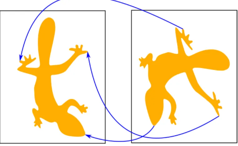
Image registration (IR) has been applied in a large number of research areas, including medical image analysis, computer vision and pattern recognition [87]. The goal of IR is to find a geometric, or elastic transformation that makes one image similar to the other (Fig. 3.1) [28]. In all IR problems, there are at least two images, a Static (S ) and Deformed (D), that represent the same object, or scene viewed from a different perspective, and/or with different deformation. Defining it more formally, IR aims to find the best mapping function T to warp D towards S, as shown below:
W = T (D)≈ S . (3.1)
W is a warped image that should be as closely shaped to S as possible. IR typically has the four following steps [87]:
1. Feature detection; 2. Feature matching;
3. Mapping function design;
4. Image transformation and re-sampling.
In order to find the correct transformation, image features such as closed-boundary re-gions, edges, line intersections, corners, and so on, should be extracted (feature detection). These features can be used as control points. Correspondences have to be set between the extracted features of S and D (feature matching). Then, the type of transforming model has to be chosen and its parameters estimated (mapping function). Finally, D is transformed by means of the mapping function (image transformation).
Figure 3.1: Finding a transformation by point correspondence.
IR can be seen as a function approximation method [78], and it is a NP-Complete problem [53]. The most important aspect of parametric IR is the discovery of the un-known parametric transformation that relates the two images. Two different approaches can be found in the literature:
• Matching-based approaches
• Transformation parameters-based approaches
Matching-based approaches conduct a search within the space of possible feature correspondences (typically point matching) between the two images. Thereafter, the parameters for the transformation are calculated based on the correspondence found.
3.2. Warping 33 In contrast, transformation parameters-based approaches perform a direct search in the space of the parameters of the transformation.
IR methods can also be classified according to the type of models that they allow to transform D into S (sometimes also referred in the literature as the scene and model images). Two major types of models used are: linear and non-linear transformations. Linear transformations preserve the operations of vector addition and scalar multiplica-tion. The same does not hold for non-linear (or elastic) transformations, which allow local deformations of the image.
The chapter starts by describing several geometrical warping models (or transforma-tion). The estimation of the difference between warped and static images is considered in Sect. 3.3. The chapter ends with a brief literature review of related work that has been proposed to address the IR problem, both with classical, EC and Metaheuristic (MH) methods in Sect. 3.4.
3.2
Warping
Independent from the IR algorithm, warping is a very important step in the registration process. Image warping is the application of the calculated transform to the deformed image or, in other words, the process of geometrically transforming a given image. In order to apply geometric transformations to the image, a transform function has to be defined. Transforms may be rigid or non-rigid. Non-rigid warping is also called elastic [28].
One way of applying the transformation is by transforming each position of the de-formed image D and setting the corresponding position in the warped image W , the following way:
W (T (i))← D(i) , (3.2)
warping. Another way of applying the transformation to the image, is by finding a value in the deformed image for each position of the warped image. This approach is called backward warping. Therefore, T which is used in Equation (3.2) is not suitable anymore, and the inverse of the transformation should be used the following way:
W (i)← D(T−1(i)) . (3.3)
With this approach all the positions of the warped image W are visited once.
3.2.1
Geometric Transform
A common and straightforward approach for doing IR is to deal with the deformation as if it was global. Thus, the transformation is applied globally to the image. Rotation and translation are the most common differences between static and deformed point-sets, and these, very often, affect the image globally.
Transformations that are frequently used to correct global misalignments are de-scribed in the following subsections.
3.2.1.1 Rigid
Transformation can be classified as rigid and non-rigid according to the transform used in the process of registration. Rigid transformations preserve the straightness and size of all lines, as well as the angles between them. A rigid transformation can be split in two parts, i.e., translation and rotation. The affine transform can be seen as a special case of the rigid classification which furthermore is able to do shearing.
3.2.1.1.1 Affine Transform
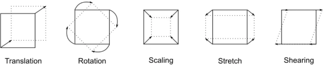
The affine transform is a linear transformation that includes the following elementary transformations: translation, rotation, scaling, stretching, and shearing [50]. These ele-mentary transformations are illustrated in Fig. 3.2.
3.2. Warping 35
Translation Rotation Scaling Stretch Shearing
Figure 3.2: Elementary geometric transforms for a planar surface element used in the affine transform: translation, rotation, scaling, stretching, and shearing.
A geometric operation transforms a given image D into a new image W by modifying the coordinates of the image points, as follows:
D(x, y)−→ W (xT ′, y′) . (3.4)
The original values of image D, located at (x, y), warp to the new positions (x′, y′) in the new image W. To model this process, we first need a mapping function T that is a continuous coordinate transform. An affine transformation function works in the 2-D space, thus, the search space is:
T : R2 −→ R2 . (3.5)
The mapping function can be redefined as:
W = T (D) T : R2 −→ R2 .
(3.6)
The warped image W (x′, y′), in the case of the affine transformation, can be specified as
the following two separated functions for the x and y components:
x′ = T
x(x, y) (3.7)
An affine transformation can be expressed by vector addition and matrix multiplication as shown in Equation 3.9, x′ y′ = S cos θ − sin θ sin θ cos θ x y + tx ty (3.9)
where S is the scaling parameter. By multiplying S with the rotation matrix, Equation 3.9 can be written as:
x′ y′ = a11 a12 a21 a22 x y + tx ty . (3.10)
Finally, by using homogeneous coordinates, the affine transformation can be rewritten as Equation 3.11. x′ y′ 1 = θ0 θ1 θ2 θ3 θ4 θ5 0 0 1 x y 1 . (3.11)
The affine transform has six parameters: θ0, θ1, θ2, θ3, θ4, and θ5. θ2 and θ5 specify the
translation and θ0, θ1, θ3, and θ4 aggregate rotation, scaling, stretching, and shearing.
3.2.1.2 Non-Rigid
Non-rigid transforms, also called deformable and elastic, allow more complex distortions in the image. These include the stretching and curving of the image. There are different kinds of transforms that are classified as non-rigid transformations, e.g., projective trans-form [45], quadratic and cubic polynomial [15], and thin plate splines (TPS) [29], just to mention a few.
3.3. Estimation of the Difference 37
3.3
Estimation of the Difference
After estimating the transformation, and warping the image, the similarity between the static image and the warped image should be evaluated in order to assess the quality of the registration. This is a crucial step if image registration is done automatically, and not by manually selecting and placing landmarks. There are many choices for similarity estimators. The sum of squared differences is probably the most commonly used. It is defined ∀~x ∈ S ∩ W by the following equation:
SSD(S, W ) =
N
X
i
(S(~x)− W (~x))2 , (3.12)
where N is the number of points under analysis. The SSD is often normalized by dividing it by N, resulting in the mean squared error (MSE) as follows:
MSE(S, W ) = SSD(S, W )/N . (3.13)
The SSD and MSE measure the distances’ difference between corresponding points in two images, thereafter, it is equal to 0 when two similar images are perfectly aligned and increases as misalignment increases. When the images to be registered differ only by geometry and/or Gaussian noise, the SSD is a well suited similarity measure [81].
3.4
Related Work
There are a variety of techniques for solving IR problems. This section presents a brief re-view of some of the most important ones, including both classical, as well as evolutionary computation and metaheuristic (MH) based approaches.
3.4.1
Classical Methods
Two state-of-the-art approaches from this category of methods are Robust Point Match-ing (TPS-RPM) [17], and Shape Context (SC) [8].
TPS-RPM is a method for matching two point-sets in a Deterministic Annealing (DA) setting. It uses a fuzzy-like matrix instead of a binary permutation matrix to find the matching between two sets of points. In TPS-RPM, both the point correspondences and the transformations are computed interchangeably. Therefore, RPM can be viewed as a general framework for point matching and can accept different transformation models [17] like affine, and even more complicated models like Thin Plate Splines (TPS) [29]. This method is a kind of a hybrid in the sense that it can be considered both a matching-based and a transformation-based approach for IR.
Shape Context (SC) is a matching-based approach that is usually used to estimate the transformation between two images, by finding matches between samples from the edges of the objects in the images. It basically consists of analyzing the spacial relationship between points. It uses four main parameters. The first defines the number of radial bins for the creation of the histograms, the second is the number of theta bins that defines how many slices the histograms should be divided into, and the third and fourth parameters, the minimum and maximum width of the bins, respectively. For more information on these and other classical IR methods, the reader is directed to [15, 18, 87].
3.4.2
EC and MH methods
Evolutionary Algorithms (EAs) and other metaheuristics (MHs) methods have been ap-plied to solve IR problems. EAs and MHs are stochastic optimization methods which aim at finding a solution or a set of solutions that perform(s) best with respect to a certain objective(s). During the last decades these algorithms have been successful in solving a variety of search and optimization problems, and the domain of image registration has
3.4. Related Work 39 been no exception. As opposed to the classical methods, which are typically based on gradient-based search, EAs and MHs tend to escape more easily from local optima and can be considered, in general, robust methods.
The first known application of evolutionary computation to image registration is due to Fitzpatrick et al. [33] who applied a genetic algorithm (GA) to relate angiographic images. For the subsequent 15 years or so, other EC approaches have been proposed by different authors, but most of them were based on the canonical GA with proportionate selection and a binary representation for solutions. Such a GA has severe limitations when solving optimization problems in the continuous domain, especially due to the problem of Hamming cliffs originated from the discretization of real valued variables into binary coded values, to the fixed precision that depends on the number of bits used for each decision variable, and for imposing lower and upper bounds for a variable’s value. Moreover, it is known for several years that fitness proportionate selection methods have several drawbacks when compared to ordinal-based selection methods such as ranking, tournament, or truncation selection [41]. Nonetheless, most of the early EC approaches for IR used such kind of GA setup [79, 80, 38, 85, 86]. Another limitation of the early approaches was that they only dealt with translation and rotation [33, 38, 47, 85], ignoring scaling, stretching, and shearing.
Most modern EC applications to IR use a direct real coded representation of so-lutions [66, 47, 39, 16, 19, 84, 78]. Besides EC, other MH approaches have been ap-plied to IR, namely Tabu Search [82], Particle Swarm Optimization [83], Iterated Local Search [21], and Scatter Search [20, 70] just to name a few. A detailed review of these works cannot be made in this thesis, but the interested reader can consult recent surveys on the topic [22, 69].
Chapter 4
Application of Evolutionary
Algorithms to Image Registration
4.1
Introduction
This section introduces a real coded genetic algorithm for the optimization of the param-eters of an affine transformation for the case of 2-D images. The proposed algorithm is a transformation parameters-based approach, since we are performing a direct search for the parameters that define the registration transformation. For the sake of simplicity, we assume we have two 2-D synthetic point-sets representing features from the two images. In other words, it is assumed that the feature detection step of the IR pipeline has been solved beforehand. The problem undergoes two different evolutionary algorithms, ES and GA. In the next sections, the representation, the operators, and the objective function that were used in this study are described.
In this chapter, the new noisy objective function is proposed (Sect. 4.3). Sect. 4.4 presents a real coded GA formulation and operators for the IR problem. The experimental results of the GA formulation are presented and discussed in Sect. 4.4.1. Once the ES is more used for continuous search space, it was also applied to the problem at hand.