E
CONOMETRIA
A
PLICADA E
P
REVISÃO
T
RABALHO
F
INAL DE
M
ESTRADO
D
ISSERTAÇÃO
U
NDERSTANDING THE
P
ORTUGUESE
U
NIT
L
ABOR
C
OSTS
L
UÍS
F
ILIPE
Á
VILA DA
S
ILVEIRA DOS
S
ANTOS
O
RIENTAÇÃO:
P
ROFESSORD
OUTORM
ÁRIOC
ENTENOi
ABSTRACT
This paper analyzes the effects of monetary policy and financial variables over Portuguese firm-level Unit Labor Costs (ULCs), between 2006 and 2009. It focuses on log-decomposing ULCs, as wages, number of employees, value added and price deflator, allowing isolating the main contributors for the overall effect.
ii
RESUMO
O presente artigo analisa os efeitos da política monetária e das variáveis financeiras sobre os Custos do Trabalho por Unidade Produzida (CTUPs), ao nível das empresas Portuguesas, entre 2006 e 2009. Dá-se especial enfoque à decomposição logarítmica dos CTUPs, enquanto salários, número de trabalhadores, valor acrescentado e deflator de preços, permitindo isolar o principal contribuinte para o efeito global.
iii
ACKNOWLEDGMENTS
I would like to thank all the economists and associates with Economic Research Department of the Bank of Portugal, especially to my advisor Mário Centeno for his availability, support and encouragement. I also would like to thank Ana Soares, Maria Teresa Nascimento, Paulo Rodrigues, Álvaro Novo, Fernando Martins and Cláudia Duarte, for their crucial suggestions, comments and methodological guidance, and Lucena Vieira for the data support.
Special thanks to Isabel Proença and Maximiano Pinheiro, professors of the Applied Econometrics and Forecasting master program, for their availability, comments and suggestions.
I could not forget my Family, my Girlfriend, Joana Raminhos, and my closest Friends for their comprehension, motivation, support and love in every single moment.
Finally a great thank to my master’s colleagues, especially to Ana Sequeira, a partner in this journey, for every day enthusiasm, motivation and affection.
Thank you all,
iv
C
ONTENTS1. INTRODUCTION ... 1
2. LITERATURE REVIEW ... 2
3. DATA DESCRIPTION... 5
3.1. Merged Datasets... 5
3.2. Data refinements ... 9
3.3. Descriptive statistics ... 11
4. ECONOMETRIC FRAMEWORK ... 11
4.1. Models’ characterization and the decomposed Unit Labor Costs ... 12
4.2. Static Model ... 15
4.3. Cross-Sectional analysis ... 18
4.4. Dynamic Model ... 19
5. EMPIRICAL RESULTS ... 25
5.1. Static Model ... 25
5.2. Cross-Sectional analysis ... 27
5.3. Dynamic Model ... 29
6. ROBUSTNESS CHECKS... 32
7. CONCLUSIONS AND FUTURE RESEARCH ... 35
REFERENCES ... 36
APPENDIX A–TABLES AND FIGURES ... 41
APPENDIX B–VARIABLES DESCRIPTION... 45
v
L
IST OFT
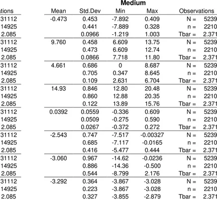
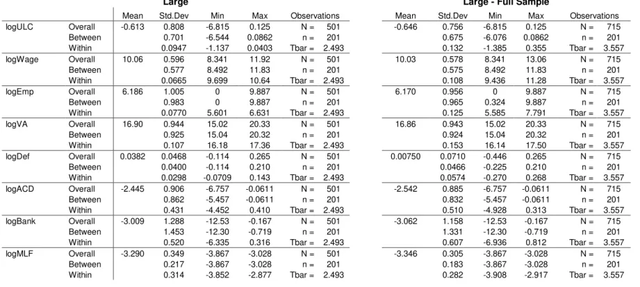
ABLESTable A.1 – Descriptive Statistics for Small and Medium firms, variables in levels ... 41 Table A.2 – Descriptive Statistics for Large firms, IES sample (2006-2009) and Full sample (2003-2009), variables in levels ... 42 Table A.3 – Number of Firms in sample, from 2006 to 2009, by Sector ... 42
Table C.1 – Static Model: Fixed Effects versus Between Effects ... 46 Table C.1.1 – Hausman specification tests, based on the classical (non-robust) and Wooldridge’s (robust) versions ... 47
Table C.2 – Cross-Sectional analysis: Seemingly Unrelated Regression (decomposed ULC) and Ordinary Least Squares (ULC equation) ... 48 Table C.2.1 – For Small and Medium firms ... 48 Table C.2.2 – For Large firms ... 49
Table C.3 – Dynamic Model for the log-decomposed ULC: Pooled Ordinary Least Squares and Fixed effects ... 50 Table C.3.1 – Estimations with the logarithm of Apparent Cost of Debt ... 50 Table C.3.2 – Estimations with the logarithm of Bank’s interest rate for Short Run and Long Run loans ... 51 Table C.3.3 – Estimations with the logarithm of Marginal Lending Facility ... 52
vi
L
IST OFF
IGURES1
1. INTRODUCTION
Discussions about the ways of improving competitiveness within the European countries are currently the main concern of political authorities, to promote economic growth and to reduce financial markets’ pressure over sovereign debt, especially after the Euro adoption. Such debate fall in the discussion of country-level Unit Labor Costs – hereinafter ULC(s) –, total labor compensation to labor productivity, i.e. total labor cost per unit of output, interpreted as a measure of competitiveness.
Countries can adjust their ULC by promoting overall labor productivity (measured as real value added to workers), but also by reducing the total cost of labor, which can be quite oppressive, for the workers side. Besides, the adjustment through capital can also affect competiveness. The question is: which one grows faster, i.e. does the nominal wage grows faster than the labor productivity or, on the other hand, does nominal profit rate decreases slower than capital productivity?
Since the ULC can be interpreted as a synthetic index of competitiveness, it hides several specific characteristics as nominal rigidities (prices and wages), but also quantity rigidities (labor), both likely to constrain the monetary transmission mechanism. Consequently, it emerges as a rigid competitiveness index. Therefore, decomposing the ULC allows isolating specific dynamics and should minimize combined rigidities effects.
2
This study focuses on the analysis of annual Portuguese firm-level data, contributing to the state of art with an extensive investigation about how Portuguese firms’ ULCs react to the monetary policy and to other financial variables, evaluating how effective the monetary transmission mechanism is, in terms of competitiveness.
We aim at combining typically microeconometric analysis with macroeconometric frameworks, in terms of the multipliers analysis (average short run and average long run effects).
Taking into account the characteristics of the Portuguese firms, we will separately analyze them considering their different size – Small, Medium and Large firms –. However, we will implement the same model to explain these “universes”.
Marques et al. (2010) and Druant et al. (2009) show us that the Small firms are likely to be less rigid, relatively to the Large ones, and also slower in adjustments to monetary shocks, so we might expect that the Small firms’ ULCs might display a lengthened response and, therefore, less constraints for the monetary transmission.
The remainder of this paper is organized as it follows: section 2 provides a review of relevant literature, while section 3 describes data and their refinements. Sections 4 and 5 present empirical methodologies and the results, respectively, while section 6 presents the robustness checks performed. Finally, section 7 concludes.
2. LITERATURE REVIEW
3
Algebraically, the economy’s ULC, in period t, can be described as it follows: w L LaborCompensation
ULC p p LaborShare p
VA VA
×
= × = × = × (1)
by log-linearizing equation (1), we get:
(
)
( )
( )
( )
( )
log ULC =log w +log L −log VA +log p (2) where w is the total labor compensation per worker (or just wages, even though it includes additional compensations to workers), L is the number of employees, VA is the value added and p is the price deflator (a unitless magnitude). By log-linearizing, we can isolate the driver(s) of a specific effect, over the ULC.
Especially for Portugal, it is argued that the progressive loss of competitiveness is essentially due to the price deflator growth. It might be true in aggregate level, but it does not necessarily hold for the firm level case, since the aggregate ULC does not result from a simple weighted average of each firms’ ULCs. However, we can rewrite the aggregate labor share (not ULC) as a weighted average of each firm’s labor share:
1 1
1 i i
K K
n i i i
L K L L
i i
i i
i p q
s s s
p q ϕ = = = = × =
∑
∑
∑
(3)where ϕi is the share of the th
i firm’s value added, in total value added, and sLi is the
th
i firm’s share of labor on its value added. Recalling equation (1), we can decompose the ith firm’s labor share as:
i i i i
L
i i i
w l ulc s
p q p
= = (4)
4
1 1 1
1 i i
K K K
n i i i i
L K L i
i i
i i i i
i
ulc p q
ULC s P s P P ulc
p p q ϕ ϕ = = = = = × = × × = × × ≠ ×
∑
∑
∑
∑
(5)proving the underlined difference.
Altomonte et al. (2012) also discuss the distortions that might arise from a simple aggregate analysis, due to improper weighting, pictured on a misrepresentation of a given sector or firms’ cluster (by size, labor force characteristics, and so on…). Indeed, the “average” policy effect can hide quite heterogeneous responses for some firms, even though “average” competitiveness gains; also one can be inflicting a severe cut in a growing sector or firms’ cluster, while encouraging a big saturated sector.
Knowing that the aggregate analysis might be distortive, the concept of disaggregation must be taken to another level, as the ULC summarizes three variables with an extensive literature about their rigidities: prices, wages and employment.
Marques et al. (2010) assemble micro evidences on commonly observed correlations with respect to (hereinafter w.r.t.) price rigidities: (i) in firms with high labor cost share, prices seem to change less frequently; (ii) changes in demand and in competitors prices mainly matter for price decreases, hence competition seems to reduce price stickiness, consistent with recent findings on macroeconometric literature, using disaggregated price data, as prices also respond slower to a monetary shock1; (iii) firms seem to respond faster to negative, than to positive demand shocks, however their size do not determine these adjustments, following Dias et al. (2011) results, from an Ordered Probit estimation of price adjustment lags to firms’ characteristics.
5
In terms of wages, they are also to be known as sticky. Druant et al. (2009) studied the relationship between prices and wages in European firms and their findings are straightforward: commonly, firms adjust wages less frequently than prices. Aiming at the Portuguese case, there is a positive correlation between Small firms’ flexibility and wage adjustments, contrasting with Large firms, which typically adjust through wage supplements, as they also prefer cheaper hires, potentially lowering the quantities rigidity, as advocated by Dias et al. (2012) and Centeno and Novo (2012).
These results are also widely discussed in Branguinsky et al. (2011), focusing on the Portuguese Labor Market, with high degree of labor protection and excessive government support for smaller firms, making adjustments very problematic and shifting firms’ size distribution since the 70’s. By presenting a model assuming high degree of labor protection, operating as a tax on wages, they conclude that this may cause degradation on allocated resources, potentially lowering aggregate productivity.
3. DATA DESCRIPTION
In this section, we present detailed information about all the datasets used, in this analysis, and all the refinements made, so that we have representative information about our universe, minimizing all possible bias, such as data selection or measurement errors. Finally, a brief descriptive analysis for the relevant variables is presented.
3.1. Merged Datasets
6
Banco de Portugal, and “Quadros de Pessoal (QP)”, Ministry of Labor and Social
Security, for the 2002-2009 period.
The CB and IES datasets provide information from firms’ balance sheets, while QP provides detailed information about their workers, in terms of quantities, spendings and their characteristics (years of schooling, workers experience, gender, and so on…).
CB is an annual dataset that covers the whole sectors of the Portuguese economy
since 2000, excluding the Financial Sector, Public Activities2 and Societies. It was incorporated in IES, introduced in 2006, with the objective to simplify the annual reporting to the public entities, responsible for supervision, investigation and statistical information providing. This transition allowed reducing the cost of obtaining information and expanding the statistical information to the “universe”, already in 2005, due to T−1 reporting, as a control. At that point, the statistical information was obtained from a sample of firms who provided their balance sheets to Portuguese Instituto Nacional de Estatística and Banco de Portugal.
Note that when CB-IES was merged with QP, there was a loss of about one million observations, almost a half of the total, at that point. We underline two reasons: firms report IES but do not report QP, and vice-versa. No plausible explanations were found for such behavior, due to the compulsory nature of both IES and QP.
In addition, once firms report their 5-digit “Classificação Portuguesa das Atividades Económicas (CAE), Revisão 2.1”, for the CB period, and “CAE Rev. 3”, for the IES period, we have also merged Industrial Production Price Index (IPPI) and
2
7
Consumer Price Index (CPI) annualized data, from Portuguese Instituto Nacional de Estatística, to deflate Industry and Electricity and Water firms’ ULCs and Construction,
Trade and Services firms’ ULCs, respectively. This procedure is conditional to the different CAE classification revisions reported, avoiding possible measurement errors arising from incorrect correspondences between “CAE Rev. 2.1” and “CAE Rev. 3”.
It is important to note that the existing firms in 2005 and which did not report IES-2006, are also taken into account and deflated according to “CAE Rev. 2.1”. Those
who were still observed in both 2005 and 2006 are deflated according to “CAE Rev. 3”, due to T −1 reporting of CAE, in IES-2006.
Since IPPI is referred to CAE classification, we have directly merged the information for 3-digit “CAE Rev. 2.1” firms, from IPPI base 2000 (from 2000 to 2008), and 3-digit “CAE Rev. 3” firms, from IPPI base 2005 (from 2005 onwards).
In contrast, we had to reclassify CPI, referred to 5-digit “Classificação Portuguesa do Consumo Individual por Objetivo (CCIO)”, equivalent, at 4-digit level,
to 3-digit “Statistical Classification of Products by Activity in the European Economic Community (CPA)”3. The latter has a direct correspondence with CAE at 3-digit level.
Like the IPPI, the CPI is separated in two basis year: CPI base 2002 (from 2002 to 2008) and CPI base 2008 (from 2008 onwards). But merging is not straightforward, since, in 2008, the CPI turned to be a chain index, raising some additional difficulties, in terms of regrouping the elementary indexes to the new classification4.
3 Correspondence table available at http://ec.europa.eu/eurostat/ramon (COICOP 1999 - CPA 2008). 4 The International Labor Organization provides an extensive guide to CPI methodological issues
8
Then, we have merged these two different CPI bases, reclassified in both 3-digit “CAE Rev. 2.1” and 3-digit “CAE Rev. 3”, the latter, retropolated until 2005, where:
NewBase Retrop OldBase 1
OldBase 1 t
t t
t p
p p
p +
+
= × (6)
so it can be possible to deflate the respective firms, taking into account the different classifications reported.
Note that these deflators are not firm-level, due to confidential restrictions, especially in IPPI. Therefore, unavoidable measurement errors might be a strong possibility, due to aggregation and heterogeneity omission, in sectors whose firms’ product differentiation is high or moderate.
Also, both IPPI and (reclassified and retropolated) CPI are at 2006 basic prices, once we have gathered information about the (aggregate) Gross Value Added, from Portuguese Instituto Nacional de Estatística, so we could compute firms’ weights on the aggregate, for representativity purposes.
In terms of the Monetary Policy variable, we have collected information from the European Central Bank’s marginal lending facility reference rate, available at Eurostat. The annualized data is obtained by weighting the observed value by the
number of days in which the monetary stance hold, between 2002 and 2009:
(
)
11 1
J J
MLF MLF
t j j j
j j
i i d d
−
= =
= × ×
∑
∑
(7)9
3.2. Data refinements
Firms which report turnover and assets above 1000€, strictly positive employees expenditures, at least one person employed, strictly positive capital and value added (which must be higher than total labor compensation), were included on this analysis.
However, firms which report ratios above 100%, such as Return on Equity, Apparent Cost of Debt (total financial interest expense to financial debt, including bank loans, medium and long maturity bonds, and subsidiaries loans) and Bank’s interest rate for Short Run and Long Run loans (total financial interest expense to bank loans) were excluded, which had a less than 6% impact in the overall observations.
For comparability issues, between static and dynamic models, we have imposed that the firms’ ULCs, apparent cost of debt, bank’s interest rate, turnover and return on equity must be observed at least two consecutive times. This restriction cuts observations by almost a half, especially due to the non-reporting of financial variables. Additionally, one time observation is lost.
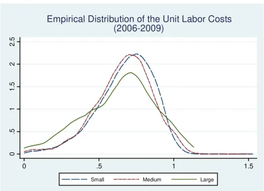
We call the attention to the fact that all of the refinements above do not severely affect the empirical distributions for the relevant variables. Nevertheless, the Micro firms were excluded due to lack of dynamics and since only the stable ones remain.
For a unique characterization of the firms’ size, during the analyzed period, we apply the following criteria:
(
)
1(
)
dimi T a 1 Tt adimit −
=
= − + ×
∑
(8)
10
preliminary analysis, we examine, in our dataset, that the probability of transitions between different firm sizes is below 6%, and it is typically a reduction in size: Medium to Small and Large to Medium. For simplicity, we consider this effect negligible, strengthened by unchanged signs and minor changes in magnitudes of the estimated coefficients, in preliminary Fixed Effects estimations.
We accommodate the sectoral changes, due to misreporting of CAE, before 2005, or changes on the main activity, by dynamic observability of firms’ ULCs. If a given firm spent most of the time in the “old” sector, then the “new” sector observations were excluded. If not, then the “old” sector observations were excluded. If a given firm spent the same time in both “old” and “new” sectors, then the observations earlier than 2005 were excluded, since there was a major revision of CAE reporting, when IES was introduced. This procedure had a 0.2% effect in overall observations.
However, a possible selection bias emerges from the CB dataset, towards the Large firms, which is straightforwardly observed when we analyze the effect of IES introduction: little impact on total number of Large firms and an exponential increasing effect, as firms size decreases.
The solution would be estimating a first step year-by-year Probit, to obtain the Inverse Mills Ratios (IMRs), as suggested by Wooldridge (2002), but there are also severe constraints to that procedure: we do not know the year that a given firm is “born” and we also do not know if the missing value is due to exit, lay-off or non-observability.
11
regressors for the periods wherein firms have already left the panel, which, in this case, are the macroeconomic variables. Therefore, even if a panel-style Probit is estimated, when constructing the IMR, using this dataset, it would be time-varying, but equal for all firms, in a given year, unlike the usual Heckman selection bias correction5.
Being aware of such additional difficulties, we will only analyze the IES period (2005-2009) and, as a robustness check, we will analyze the whole period (2002-2009), for the Large firms observed in both periods, as they are not likely to be selected. This allows us to control possible changes in the estimated signs and magnitudes.
3.3. Descriptive statistics
Based on appendix A, we present an initial descriptive analysis, for the relevant variables, in levels, and observe that: (i) as firms size increases, both average ULCs and average price deflators tend to be lower, while average wages, average number of employees and average value added follow in the opposite line; (ii) heterogeneity related to both ULCs, its components and the financial variables, tends to be higher, as firms size increases; (iii) no clear pattern for the financial variables’ averages; (iv) aggregate apparent cost of debt is always higher than any other aggregate interest rate considered, reflecting risk perception, once it covers several other ways of financing.
4. ECONOMETRIC FRAMEWORK
This section addresses the econometric methodologies implemented, based on Portuguese firm-level ULCs and their decomposition, starting with a static model and
12
respective specifications tests, to a coefficient stability cross-sectional analysis, concluding with a dynamic model and respective multipliers analysis.
4.1. Models’ characterization and the decomposed Unit Labor Costs
Due to the lack of relevant literature related to the functional form of firm-level ULCs and specifically to the relationship between competitiveness and the monetary and financial variables, we will use the log-decomposition in (2), analyzing these effects in terms of elasticities, allowing highlighting the driver(s) of the overall effect.
Our purpose is to estimate a system where the dependent variables are the log-decomposed ULC: logarithm of wages, logarithm of the number of employees, logarithm of value added and logarithm of price deflator. Separately we will estimate a model with the logarithm of ULC as the dependent variable. For each of these, we perform three different estimations including, in each, the logarithm of apparent cost of debt (logACD), then the logarithm of bank’s interest rate (logBank) and finally the logarithm of marginal lending facility (logMLF), at once. Each model is also estimated by each firms’ size.
Using this alternation strategy, we can isolate a direct monetary policy effect, from banks and financial markets influence on the monetary transmission mechanism to Portuguese firms, in terms of competitiveness.
We have also included several controls on these estimations, described in appendix B, accounting for the sensitivity of Portuguese firms’ ULCs to capital, labor and external markets.
13
(
)
, , , , ,log ULC H ULC H ULC H ULC H ULC H
it it it i t it
ULC =β H +X′δ +µ +λ +ε (9)
( )
( )
(
)
( )
, , , , , , , , , , , , , , , , , , log log log logw H w H w H
w H w H
it i t it
L H L H L H
L H L H
it i t it
it it VA H VA H VA
VA H VA H
it i t it
p H p H
p H p H
it i t
w
L
H X
VA
p
µ λ ε
β δ
µ λ ε
β δ
µ λ ε
β δ µ λ β δ = + ′ + + + , , H p H it ε (10)
{
}
,1,..., j t; 2006,..., 2009; i ; Small, Medium, Large
i= N t= T ≤T j∈ , and:
{
logACD , logBank , logMLF}
it it it t
H ∈ (11)
where each of the elements, in Hit, are alternately used in each equation, also providing different estimates considering the element used, reflecting the “H” on superscript. In equation (9) and (10), Xit is a
(
k− ×1 1)
vector of control variables. In addition, the β's are scalars and δ's are(
k− ×1 1)
vectors, on equation (9) and in each equation of the system in (10). The δ's also contain a constant term.Sectoral and time dummies have also been included, the latter with the exception for the model with the logarithm of marginal lending facility, since it is a macroeconomic variable, and so, time-varying, but equal for all firms, in a given year.
In the dynamic version we have the following:
(
)
,(
)
, , , , ,, 1
log ULC Hlog ULC H ULC H ULC H ULC H ULC H
it i t it it i t it
ULC =α ULC − +R′ψ +K′ζ +µ +λ +ξ (12)
( )
( )
( )
( )
(
)
, , , , , , , , , ,, 1 ,
, , , , , , , log log log log log
w H w H
w H w H w H
it i t
L H L
L H L H L H
it i t
i t it it VA H
VA H VA H VA H
it i
p H
p H p H p H
it i
w L
ULC R K
VA p
µ λ
α ψ ζ
µ λ
α ψ ζ
µ
α ψ ζ
µ
α ψ ζ
− = + ′ + ′ + + , , , , , , w H it
H L H
it
VA H VA H
t it
p H p H
t it ξ ξ λ ξ λ ξ + (13) ,
1,..., j t; 2006,..., 2009
14
The alternation procedure, concerning Hit elements, still holds on these estimations. In this case Kit is a
(
k− ×2 1)
vector of control variables and may contain lagged regressors. In addition, the α's are scalars, ψ's are 2 1× vectors and ζ's are(
k− ×2 1)
vectors, on equation (12) and in each equation of the system in (13). The ζ'salso contain a constant term. Sectoral and time dummies have also been included. The lagged regressors, in Rit, allows us to obtain the relevant impact multipliers.
Note that the “sum” of the estimated coefficients for each covariate, obtained from the log-decomposed ULC system in (10) and (13), is equal to the estimated coefficient for the same covariate, in the logarithm of ULC equation. For example, in (10), βw H, +βL H, −βVA H, +βp H, =βULC H, .
Even though we have information about the population, inference might be interesting, since this population can be interpreted as resulting from one realization of an independent and identically distributed (i.i.d.) process, as in macroeconometrics approaches.
We will focus on Seemingly Unrelated Regression (SUR) method, purposed by Zellner6, to estimate the systems of log-decomposed ULC, in (10) and (13). Note that each equation, on these systems, has the same set of regressors.
As shown in Hayashi (2000), by making no assumptions about the inter-equation error correlation, having common exogenous regressors in each equation and assuming conditional homoscedasticity, the Feasible Generalized Least Squares (FGLS) is
15
numerically equivalent to the efficient Generalized Least Squares (GMM) estimator, proposed by Hansen (1982). Hence, considering this framework, SUR is numerically equivalent to the efficient GMM. Likewise, Amemiya (1985) and Greene (2002) claim that SUR with common regressors in each equation is also numerically equivalent to equation-by-equation Ordinary Least Squares (OLS)7.
On the other hand, Avery (1977) and Baltagi (1980) argue that when estimating a model with error components, this condition is not sufficient for the equivalence to hold, since the composite error is autocorrelated, due to the presence of the individual effects. Besides, SUR assumes that the error for each equation is non-autocorrelated, however it can be correlated between different equations.
The latter is the case of the Random Effects (RE) estimator, since the individual effects are not eliminated, so the composite error is autocorrelated in each equation. Therefore, a Random Effects SUR is not numerically equivalent to equation-by-equation RE.
4.2. Static Model
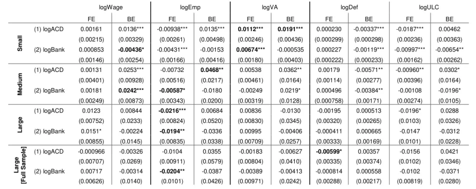
We begin with a static model using Fixed effects (FE) and Between effects (BE) estimators. Baltagi (2005) and Kennedy (2003) argue that typically FE, based on the time-series component of the data, tends to provide short run estimates, while BE, based on the cross-sectional component of the data, tends to provide long run estimates, since it is a regression on individual time-averages, i.e., a cross-sectional regression over
7 These authors provide different demonstrations of this equivalence. See also Lu and Schmidt (2012) for
16
time-averages, capturing the structural component of the data. Following this strategy, we can isolate the “short run” and “long run” overall effect, as well as their drivers.
As FE and BE are, in fact, OLS estimations of a transformed model, we extend the SUR-OLS equivalence to this case. If we perform FE estimations, the transformed error component is not autocorrelated because the individual effects are eliminated with the within transformation. As for the BE estimations, the SUR-OLS equivalence directly holds since we are performing a cross-sectional regression over time-averages.
Also, we guarantee that the estimated variances are corrected for possible presence of heteroscedasticity and autocorrelation (in the residual structure), using firm-level cluster robust standard errors (White cluster for FE and cluster bootstrap for BE, based on one hundred replications), insuring consistency of inference for both FE and BE estimations.
Note that both FE and BE provide consistent estimates if the individual-specific effect ( )µi is not correlated with the regressors, i.e., if the Hausman test, based on the differences between FE and RE estimates, lead us to the non-rejection of the null of exogeneity. However, if the null is rejected, then RE and BE are inconsistent, since both contain the individual effects and BE is a special case of RE. Additionally, this test implies that the RE estimator is more efficient than the FE estimator.
17
asymptotic normality of the FE estimator might be a “doubtful assumption”. As the Hausman test is based on the asymptotic normality of both FE and RE (and also BE), if these conditions do not hold, this test has, once again, a nonstandard limiting distribution. Furthermore, in the presence of small within variation and reduced number of observations the central limit theorem is no longer applicable.
Bearing in mind the issues above, Wooldridge (2002) suggests a similar test, inspired on Mundlak (1978) seminal paper, assuming that the time-varying regressors might be correlated with µi, in a restricted way:
(
i| i, i)
(
i| i)
0 iE µ H X =E µ w =γ +wγ (14)
where wi include time-varying regressors and
1 1 T
i T t i
− =
=
∑
w w .
The test statistic is a comparison between augmented and non-augmented RE estimations of equation (9) and each equation of the system in (10), from which we obtain the unrestricted Sum Squared Residuals and the restricted Sum Squared Residuals, respectively. Bearing in mind this formulation, the test is valid even if the homoscedastic hypothesis does not hold. If this is the case, then a robust Wald statistic is reported instead, based on Wooldridge
0 : 0
H γ= .
It should be noted that we are not interested in testing the simultaneous exogeneity of the regressors included on the whole system, in (10). Instead we want to test their exogeneity, in each equation of the system.
18
We stated the weaknesses of BE estimation, as it drops panel structure of the data, but also, in micro-panels, it is likely to be inconsistent, due to the correlation between the regressors and the individual effects. Therefore, the FE estimates might be interpreted not only as a typical “short run” (within) average effect, but also as a structural average effect, equaling the short run to the long run “multipliers”, since no lagged regressors were included, at this stage.
Considering this scenario and the purpose of this study, the next step should be towards an estimation of a dynamic model, examining the differentials between the short run and both lagged and long run effects.
4.3. Cross-Sectional analysis
Knowing that the time dummies capture time-specific effects over the dependent variable, we can extend this approach to the regressors, by interacting them with these dummies, which is equivalent to a cross-sectional OLS regression of equation (9) and the system in (10). We will estimate the static system of the log-decomposed ULC, by SUR, and the ULC equation, by OLS. This can be summarized as it follows:
(
)
, , , ,log ULC H ULC H ULC H ULC H
i t i t i t t i i
ULC =β H ×D +X′δ ×D +µ +v (15)
( )
( )
( )
( )
, , , , , , , , , , , , , , , , log log log logw H w H w H w H
i t t i i
L H L H L H L H
i t t i i
i t i t
VA H VA H VA H VA H
i t t i i
p H p H p H p H
i t t i i
w v
L v
H D X D
VA v
p v
β δ µ
β δ µ
β δ µ
β δ µ
= × + ′ × + + (16)
1,..., j; 2006,..., 2009
19
The consistency of these estimations will depend on the Hausman test results, which will be carefully interpreted, bearing in mind its limitations.
We will implement these SUR and OLS estimations using firm-level cluster bootstrapped standard errors, based on one hundred replications, as a cautious strategy, suggested by Wooldridge (2002).
Being interested in the estimation of a dynamic model, we intend to ensure the dynamic stability of time-specific effects w.r.t. ULCs and to its subcomponents. Thus, a joint test for the coefficients equality, across different years, will be performed, equivalent to a structural break test. As an example, for the first equation, the null is:
2006 2007 Cross
0 2006 2008 0 2006 2007 2008 2009
2006 2009 0
: 0 :
0
w w
w w Cross w w w w
w w
H H
β β
β β β β β β
β β
− =
− = ⇔ = = =
− =
(17)
and a similar null hypothesis is used for the remaining equation-specific betas.
Once again, this test is a comparison between a restricted and an unrestricted model, where the first corresponds to the one explained solely by control variables and sectoral dummies. A robust Wald statistic is reported, as the standard errors have been adjusted. If we reject the null, it is statistically plausible to assume that the estimated time-specific effects vary across time, inducing to possible structural breaks.
4.4. Dynamic Model
20
Bond (2002) provides a guide to dynamic micro-panel data models, such as:
, 1 , 1,..., ; 2,...,
it i t it
y =φy − +u i= N t= T (18)
starting with classical estimators, POLS and FE, are widely known to be biased and inconsistent for AR p
( )
and ADL p q(
,)
models, with p>0, especially for low or moderate T case. As, for the POLS case, the lagged dependent variable is positively correlated with the error term, while, for the FE case, the lagged transformed dependent variable is negatively correlated with the transformed error term, due to the presence of individual-specific effects, shown by Nickel (1981). However, having correlations in the opposite directions, we know that a consistent estimate would lie between them, or, at least, would not be very different.Once the problem of estimating dynamic panel data models lies in the presence of individual-specific effects, we have to perform a transformation that eliminates this source of endogeneity: first differencing8. However, Cov(∆yi t, 1−,∆vit) 0≠ .
Thus, a Two Stage Least Squares (2SLS) procedure was then purposed by Anderson and Hsiao (1982), using ∆yi t, 2− or yi t, 2− as candidates to instrument ∆yi t, 1− . Arellano (1989) found that the estimator using yi t, 2− as an instrument, rather than
, 2 i t y −
∆ , have a significantly lower variance. However, 2SLS is not asymptotically efficient, as it assumes homoscedastic disturbances.
8 Within, Between and RE transformations do not eliminate this source of endogeneity, as the transformed
21
Consequently, Arellano and Bond (1991) suggested towards GMM, a suitable framework for efficient estimation, especially if the entire set of available instruments (in levels) is used, commonly known as the Arellano-Bond (AB-GMM) estimator.
As we are interested in the estimation of φ, Blundell and Bond (1998) discuss the weak performance of AB-GMM, when φ is near unity. It is clear that, in this case, we have “weak” instruments – the instruments (referred to levels) are weakly correlated with the regressors (referred to first differences) –.
Blundell and Bond (1998) purposes additional moment conditions, based on a steady state distribution for the initial condition, yi0, estimating a system where differences are instruments for the levels equation and levels are instruments for the first differences equation (Sys-GMM). This strategy was especially helpful in improving efficiency, when φ 1, attenuating the effects of “weak” instruments presence.
Moreover, if one might be looking to further efficiency, then should proceed to compute the optimal GMM weighting matrix. Windmeijer (2005) purposes a variance correction for the two-step GMM procedures, as the variance estimator is downwards biased, due to the optimal weighting matrix estimation using first-step residuals. This correction is especially appropriate for Arellano-Bond and Blundell-Bond type of instruments.
22
Roodman (2006, 2009) presents two techniques in reducing the instrument count: using a subset of lags instead of the entire set, as Wooldridge (2002) also suggests, and/or collapsing the blocks of the instrumental matrix9, once the instrument growth becomes linear-in-T .
The main concern about the instrument proliferation is related to the power of the over-identifying tests10, especially Hansen, which is robust to the presence of heteroscedasticity, but can be weakened by many instruments. Roodman (2009) argues that combining both techniques would have significant impact on Hansen tests power, not affecting the estimated coefficient, neither the estimated standard errors.
For unbalanced panels, Roodman (2006, 2009) also suggests using the forward orthogonal deviations11 equation, purposed by Arellano and Bover (1995), instead of the first differences equation, since the loss of observations is not so severe.
Bearing in mind all the issues emerging from this GMM setup and ULCs appearing to be quite persistent, as a result from preliminary POLS estimations, we will run a two-step Sys-GMM estimation for the logarithm of ULC equation, in (12), with Windmeijer corrected standard errors, considering the following moment conditions:
(
)
{
}
{
}
(
)
{
}
{
}
(
,)
{
}
,
0, for each 2006,..., 2 and 2008, 2009 ; 1,...,
0, 2007,..., 1 , for each 2008, 2009 ; 1,...,
0, 2006, for each 1 3; 2008, 2009 ; 1,...,
is it j
i
is i it j
i
i t j it j
i t
y v s t t i N
y v s t t i N
m v t j j t i N
µ − ∆ = = − = = ∆ + = = − = = ∆ = − ≥ ≤ ≤ = = ∆
∑
∑
∑
(
)
{
}
, it i it 0, 2008, 2009 ; 1,..., j
i t m µ v t i N
+ = = =
∑
(19)9 Using Holtz-Eakin et al. (1988) and Arellano and Bond (1991) full set of moment conditions. 10 See also Sargan (1958) and Hansen (1982).
11
(
)
, 1 ... ; 2006,..., 2008;
1 1
it it i t iT i
i
i i
y T t y y y t T T
T t T t
⊥
+
= − − + + = ≤
23
where mi contains all regressors (and controls), except the lagged dependent variable. As in Windmeijer (2005), mi instruments sub-matrix is collapsed, unlike the instrumental sub-matrix including lags and first-differences of the dependent variable.
As for the system of log-decomposed ULC, in (13), we will use the same equation-by-equation strategy. In this case, the model becomes a DL q
( )
, with q>0. For POLS and FE estimations, it may be arguable that the lagged logarithm of ULC might contain information about the dependent variable and so a source of endogeneity still prevails, however, no significant changes were found, using equation-by-equation Pooled 2SLS and FE-2SLS.Emphasizing again in the logarithm of ULC equation, in (12), we will focus on the Hansen test and the statistical significance of the estimated dynamic effects, commonly known, in the macroeconometrics literature, as the impact multipliers.
Taking into account the time dimension of the model, one might think about how the expected value of the logarithm of ULC evolves along the years. The contemporaneous effect is straightforwardly obtained from the estimation, but obtaining the one-step and the long run multipliers requires to rewrite the model as a DL
( )
∞ .For the one-step ahead multiplier, ∂log
(
ULCi t, 1+)
∂Hit, we have:(
)
(
)
(
)
(
)
(
)
(
)
(
)
(
)
(
)
, , , ,
, 1 0 1
, , , ,
0 1
1
, , , ,
0 1
log log (...)
1 log (...)
log 1 (...)
ULC H ULC H ULC H ULC H
it i t it it
ULC H ULC H ULC H ULC H
it it it
ULC H ULC H ULC H ULC H
it it it
ULC c ULC L H
L ULC c L H
ULC L c L H
α ψ ψ
α ψ ψ
α ψ ψ
− − = + + + + ⇔ ⇔ − = + + + ⇔ ⇔ = − + + + (20)
24
(
)
(
, , , 2)
(
,)
1 ,0 1 2
log ULC H ULC H ULC H ... 1 ULC H ULC H (...)
it it it
ULC = θ +θ L+θ L + H + −α L − c + (21)
combining (20) and (21) polynomials over Hit:
(
) (
) (
)
(
)(
) (
)
1
, , , 2 , , ,
0 1 2 0 1
, , , , 2 , ,
0 1 2 0 1
, , , , , , 2 , ,
0 1 0 1 0 1
... 1
1 ...
... ...
ULC H ULC H ULC H ULC H ULC H ULC H
ULC H ULC H ULC H ULC H ULC H ULC H
ULC H ULC H ULC H ULC H ULC H ULC H ULC H ULC H
L L L L
L L L L
L L L L
θ θ θ α ψ ψ
α θ θ θ ψ ψ
θ θ α θ α θ ψ ψ
−
+ + + = − + ⇔
⇔ − + + + = + ⇔
⇔ + + − − − = +
(22)
equating coefficients of the same power in L, yields:
, , , ,
0 0 0 0
, , , , , , , ,
1 1 0 1 1 0
ULC H ULC H ULC H ULC H
ULC H ULC H ULC H ULC H ULC H ULC H ULC H ULC H
ψ θ θ ψ
ψ θ α θ θ ψ α ψ
= =
⇔
= − = +
(23)
where ULC H, , 0,1
{ }
s s
θ = refer to the -steps multiplier.
For the long run multiplier, we evaluate all the variables at the, so called, “steady state”, described with asterisks:
(
)
(
)
(
)
* , , * , * , * 0 1 , , ,* 0 1 *
, , ,
log log (...)
1
log (...)
1 1 1
ULC H ULC H ULC H ULC H
ULC H ULC H
ULC H
ULC H ULC H ULC H
ULC c ULC H H
c
ULC H
α ψ ψ
ψ ψ
α α α
= + + + + ⇔
+
⇔ = + +
− − −
(24)
and the long run multiplier is:
(
*)
, , , 0 1 * , log 1ULC H ULC H
ULC H ULC H
ULC H
ψ ψ λ
α
∂ +
= =
∂ − (25)
Recalling the one-step multiplier, the null is 1 Step ,
0 : 1 0
ULC H
H − θ = , and for the long run multiplier, the null is LRM ,
0 : 0
ULC H
25
In terms of the log-decomposed ULC system, in (13), the one-step and long run multipliers are equal, once there is no lagged dependent variable in each equation. Thus, the null simplifies to a linear restriction. Focusing on the logarithm of wages equation,
we have: LRM , , , ,
0 : 1 1 0 0
w H w H w H w H
H λ =θ =ψ +ψ = . Once again, we can highlight the statistically significant “driver” for the short and long run overall effects.
5. EMPIRICAL RESULTS
In this section the main results will be presented and interpreted, accounting for theoretical relationships and the addressed econometric methodologies. The following sub-sections are organized as in the previous section: Static Model, Cross-Sectional analysis and Dynamic Model.
5.1. Static Model
As described before, the FE and BE estimators tend to give us different information about the underlying variables: typically we get the time-series and the cross-sectional structure of data, respectively, and so “short run” (within) and “long run” (between) estimates.
Note that the model with marginal lending facility will not be considered. Recall that this is an individual constant variable and its coefficient would not be identified on BE.
26
In a preliminary analysis, we can observe the statistical and numerical importance of the value added on the Small firms’ ULCs. However, for Medium and Large firms, this statistical and numerical importance changes towards the Labor Market variables.
On the other hand, price deflator stands typically to be the lowest contributor to the overall effect, reflecting a possible aggregation bias due to the non-observability of firm-level deflators, as firms’ ULCs are deflated by CAE 3-digit level prices, hiding significant heterogeneity for firms with high or moderate product differentiation.
Focusing on the logarithm of ULC equation, for FE estimations, we underline the highest “short run” average elasticity (in absolute value) of apparent cost of debt w.r.t. ULCs, for Large firms (0.02%), followed by Medium and Small firms (0.01%), all significant at 10%. For the model with the logarithm of bank’s interest rate there are no statistically significant effects to account.
FE estimates corroborate with the literature, since the “short run” (within) estimated elasticities have the expected signs, for all equations. Furthermore, Large firms are likely to be contemporaneously more elastic to monetary and financial variables than Medium or Small firms. However, for BE estimates, this pattern does not hold, since the estimated signs and magnitudes are quite dubious, once we denote several differences in comparison to, what is meant to be, the consistent estimator.
27
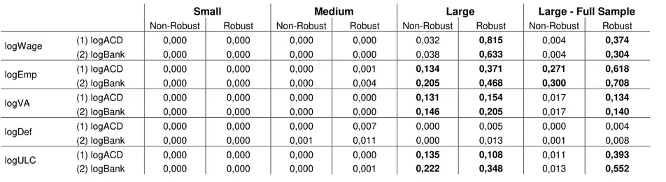
Yet, for Large firms, this test leads us to ambiguous results: in the classic and Wooldridge’s version we typically do not reject the null, which is not very plausible, compared to the previous results. Also, when analyzing the full sample period for the same set of firms (last column), this ambiguity turns out to be even greater, as we typically reject the null, for the classic version of this test, contrasting with the Wooldridge’s version, where we typically do not reject the null.
As discussed by Hahn et al. (2011), Hausman specification tests might have a nonstandard limiting distribution, in the presence of small within variation (and reduced number of observations)12. So, a careful interpretation of the p-values is recommended, since the within variation of the included regressors appears to be quite low, for all firms’ dimensions, as we can see in the descriptive statistics, from tables A.1 to A.2.
Considering such problems, we can only rely on FE consistency, which stands for both “short run” and structural model, clearly insufficient in terms of the multipliers analysis. Additionally, we account for the lack of statistical significance, concerning the Large firms estimations, which might be due to the small within variation combined with the reduced number of observations, producing very imprecise estimates.
It is clear, by now, that the drivers of the monetary and financial variables w.r.t. firms’ ULCs are not exactly the same, given different firms size.
5.2. Cross-Sectional analysis
In this sub-section, we will analyze the results from the estimation of equation (15) and the system in (16). Here, our main interest is to scrutinize statistical evidence
28
towards dynamic stability of the monetary and financial estimated effects w.r.t. firms’ ULCs.
Once again the marginal lending facility will not be included, since it is constant across firms. Also, for 2006, the coefficients from the logarithm of the price deflator equation are not identified, once the dependent variable is evaluated at 2006 basic prices, and so, constant for all firms (equal to one).
Recalling the previous results for the Hausman test, it will imply that SUR is inconsistent, due to the presence of a relevant unobserved variable ( )µi .
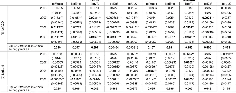
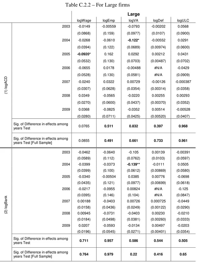
However, the year-by-year results, displayed on tables C.2.1 (for Small and Medium firms) and C.2.2 (for Large firms, IES period and full sample period), corroborate with the FE results, presented in the previous sub-section. Once again, Hahn et al. (2011) findings might help to understand this unlikely coherency.
In addition, we highlight the statistical and numerical importance of the value added, among different years, for Medium firms, which could contrast with the previous (static model) results, but a deeper analysis brings our attention to wages as the second statistically significant most important contributor to the overall effect.
Focusing on the implemented test, we typically do not reject the null, described in equation (17). Hereupon, these effects seem to be stable among different years.
29
A detailed analysis brings or attention to the (non-statistically significant) estimated elasticities for the number of employees’ equation, which dramatically changes among different years, in both estimations with the apparent cost of debt and the bank’s interest rate, severely influencing the overall effect. Even if we interpret this result as a possible structural break, due to changes in the monetary stance, the inclusion of time dummies in the panel-style estimations would be enough to capture it.
As for the remaining, once again we account for several statistical significance issues, especially for Large firms’ estimations. Also, the price deflator stands as the lowest contributor to the overall effect.
It could be argued that the statistical inference can be contaminated by the lack of bootstrap replications, especially for Small firms’ estimations. However, these results are robust to changes in the number of bootstrap replications (five hundred, one thousand and ten thousand).
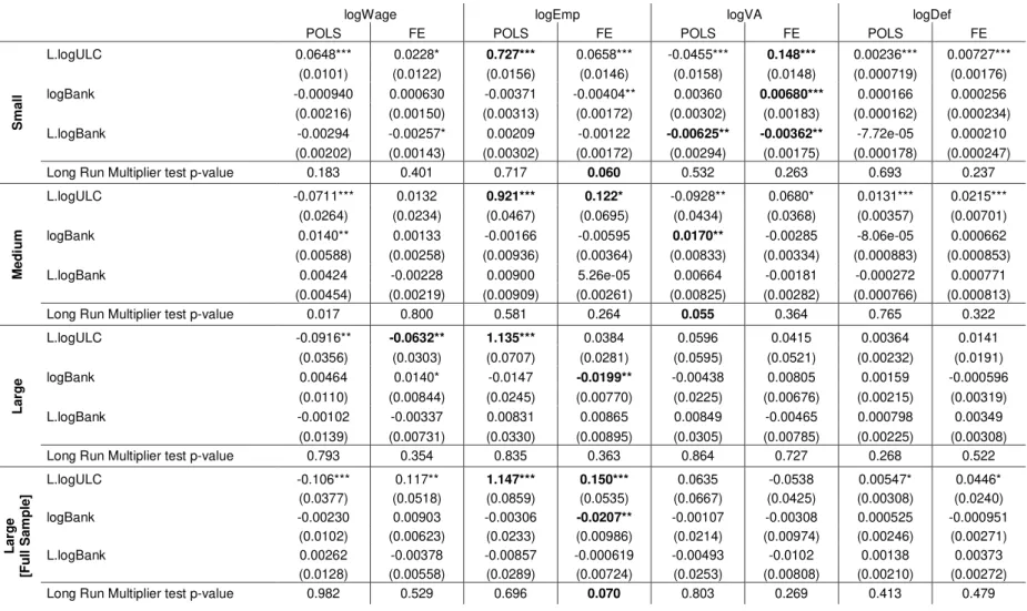
5.3. Dynamic Model
As stated before, a dynamic analysis would be enriching in sense that one can evaluate how a policy effect can prevail over time. Even though the lagged term reflects inter-year effect w.r.t. Portuguese firms’ ULCs, it might be quite informative, if there are firms that have not adjusted within the same year, which is likely to be the case for the Small firms.
30
model with the logarithm of marginal lending facility, by each firms’ size. The inconsistency of these estimates might be arguable. However, Pooled 2SLS and FE-2SLS estimates do significantly differ from these ones13. Also, these results corroborate with the FE estimation results, previously presented.
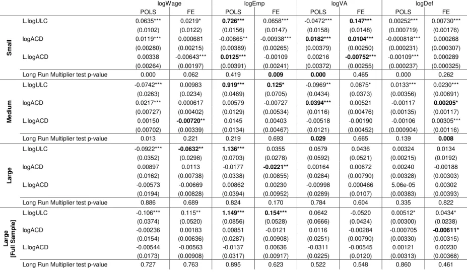
In terms of ULC persistence, typically the number of employees stands to be the highest statistically significant contributor, for both POLS and FE estimations. Concretely, for POLS, the number of employees seems to vary in the same proportion, on average, to a percentage variation on lagged logarithm of ULC, inducing to a possible presence of a unit root, on ULCs.
Even if we assume this possibility, we cannot test it with T =4, once panel unit root tests assume T ≥6 for all individual units. Additionally, FE estimations with highly persistent variables produce very noisy estimates, compared those from POLS, as the within transformation removes (persistent) time effects, almost zeroing out the transformed variable, as we can see on tables C.3.1 to C.3.3.
Concerning the short run effect, the value added stands as the driver for the Small firms’ overall effect, in the model with apparent cost of debt, and the driver for the Medium firms overall effect, in the model with marginal lending facility. This pattern holds in both POLS and FE estimations. However, for Small firms, the positively estimated signs do not seem to be coherent with the literature.
As for the long run effect, this pattern holds just for the POLS estimation of the model with the apparent cost of debt, also with (implausible) positive estimated signs.
31
Not surprisingly, for the model with marginal lending facility, the price deflator typically arises as the long run driver, in both POLS and FE estimations, for all firms’ dimensions, coinciding with price growth controlling policy of ECB.
Relatively to Labor Market variables, wages emerge, once again, as the second statistically most important contributor to both short and long run overall effect, especially for Medium firms.
Recalling the inconsistency of both POLS and FE, if we estimate an AR p
( )
or anADL p q(
,)
model, with p>0, like the logarithm of ULC equation, in (12), our choice will be towards a consistent (and efficient) GMM estimation, already defined as (two-step) Sys-GMM. Notwithstanding, we will also estimate equation (12) using POLS and FE, interpreted as upper and lower bounds for the consistent estimates, which should lie between them or, at least, should not be too far away.The major disadvantages, of this GMM procedure, are denoted by its sensitivity to moment restrictions14. In the end of appendix C, we discuss the instrumentation strategy that provides the most stable estimates.
Results are presented on tables C.4.1 and C.4.2, where the statistical significance is clearly concentrated in Small firms’ estimations. Mainly, Hansen tests do not reject the null of correct moment restrictions, after controlling for possible overfitting biases.
Introducing the autoregressive term in the estimations widens statistical significance problems and dominates other effects, as the average estimated persistence for the ULCs is above 0.8, for Medium firms, and above 0.9, for Large firms, all
32
significant at 1%. Therefore, it could have been enough estimating an AR
( )
1 model,instead of an ADL
( )
1,1 .Focusing on Small firms, solely the estimated persistence and short run elasticities are statistically significant. Nevertheless the lagged elasticities are also statistically significant, both one-step ahead and long run multipliers tests do not lead us to the null rejection, so these effects are actually not statistically significant at 10%. Since the monetary policy effects are known to not last longer than a year, the non-statistical significance of the impact multipliers seems to be reasonable.
Surprisingly, the highest estimated short run elasticity, in absolute value, is obtained by the model with the marginal lending facility (0.03%), followed by the apparent cost of debt (0.02%) and finally by the bank’s interest rate (0.008%). Both signs are consistent with the literature, but the magnitude, especially for the model with the marginal lending facility, seems to be unreasonably high, hence this effect might be contaminated with time effects, due to the time dummies exclusion, for this model.
We highlight an interesting pattern, arising from the Sys-GMM estimations: the persistence estimates are close to those from POLS, while the elasticities estimates are close to those from FE.
6. ROBUSTNESS CHECKS
33
We start our robustness checks, by disaggregating the included firms, to a sectoral and size dimension. Using the same alternation strategy, but this time, by each sector and firms’ size, we intend to investigate if there is any sector, whose (individual) estimated effect significantly differs from the (joint) size-only estimated effect. However, due to the lack of observations, only the Small and Medium firms’ models were estimated. Besides, there is no significantly different effect to be accounted. Considering the descriptive analysis, in section 4, these results were expected, since the Large firms stand as the most heterogeneous.
Next, we tried to implement an approximate version of the methodological criteria, described in section 4, for the sample based quarterly balance sheet dataset, in order to investigate if there is any time-aggregation bias on the yearly estimated elasticities. However, the number of relevant observations was less than one thousand and the Large firms were clearly over-represented. No estimations were performed.
Focusing on the missing values in the financial variables, we have engaged on an imputation strategy, following three schemes: (i) by CAE (at 3-digit level) average; (ii) by year average; (iii) combining (i) and (ii). Surprisingly, following these strategies, the results deteriorated, especially in terms of statistical significance.
Finally, repeating the estimations, considering other functional forms, produced no significant improvements over the previous results.
34
We present a proposal, based on non-linear models assumption of Correlated Random Effects: if a non-linear dynamic model, augmented by the Chamberlain-Mundlak device15, produces consistent estimates, then we would expect these good properties to hold, in the linear case, when assuming that the time-varying regressors and an initial condition, yi0, (since we are talking about a dynamic model) might be correlated with µi, in a restricted way. Recalling the Wooldridge’s version of the Hausman test16, a similar approach was used, however, for a static model.
Regarding this dynamic approach, we will consider the following model for the unobserved heterogeneity:
0 0
i yi i ai
µ γ= +θ +zγ+ (26)
assuming both time-averaged regressors and initial condition to be strictly exogenous.
We ran preliminary POLS regressions, for the logarithm of ULC equation, in (12), augmented by the Chamberlain-Mundlak device, described in equation (26):
, 1 0
it i t i i i i it
y =φy − +zβ+θy +z γ+ +a υ (27) where yit =log
(
ULCit)
, zi ⊃{
R Ki, i}
and yi0 corresponds to the logULC value for the first year that a given firm is observed. We assume strict exogeneity, in terms of the composite error ai+υit. Even though this is a very strong assumption and(
i t, 1 i)
0E y −a ≠ , this approach produces persistence estimates lying between those from POLS and Sys-GMM, and elasticities estimates between FE and Sys-GMM ones. No simulations were made. Hence, discussions about the bias order remain unclear.
35
7. CONCLUSIONS AND FUTURE RESEARCH
In this study we have investigated the relationship between Portuguese firm-level ULCs and the monetary and financial variables. In the case of an active monetary policy from the ECB, Portuguese authorities should aim at promoting demand policies, stimulating the GDP growth, driver of the Small firms’ ULCs. Consequently, we would expect a potential increase on aggregate competitiveness, if the reduction in Small firms’ ULCs is greater than in the other countries or exporting markets, as a result from a positive variation in several interest rates.
Furthermore, micro policies should be encouraged and aimed to a specific sector or firms’ cluster, due to heterogeneous and/or quicker adjustments to monetary and financial shocks, like the Medium and Large firms, once their ULCs are expected to be driven by the Labor Market variables, typically known to be highly rigid. Hence, flexibilizing the Portuguese Labor Market may produce a desirable outcome for such firms, especially in terms of competitiveness.
Contrasting with country-level literature, these effects do not seem to be driven by CAE 3-digit price deflators. However, this conclusion might not hold, if we had firm-level price deflators.
Finally we propose further investigation on Portuguese firm-level ULCs, introducing rigidity indicators in the estimated models, widely reflecting Portuguese Labor Market conditions, attenuating potential functional form misspecification.
36
REFERENCES
[1] Altomonte, C., T. Aquilante and G. Ottaviano (2012). New competitiveness indicators: firm-level evidence from the EFIGE project. Mimeo. Brussels, March.
[2] Amemiya, T. (1985). Advanced Econometrics, Cambridge, Massachusetts: Harvard University Press.
[3] Anderson, T. W. and C. Hsiao (1982). Formulation and estimation of dynamic models using panel data. Journal of Econometrics 18, 47–82.
[4] Arellano, M. (1989). A note on the Anderson-Hsiao estimator for panel data. Economic Letters 31, 337-341.
[5] Arellano, M. (2003). Modelling Optimal Instrumental Variables for dynamic panel data models. Working paper 0310, Centro de Estudios Monetarios y Financieros, Madrid
[6] Arellano, M. and S. Bond (1991). Some tests of specification for panel data: Monte Carlo evidence and an application to employment equations. Review of Economic Studies 58, 277-297.
[7] Arellano, M. and S. Bond (1998). Dynamic panel data estimation using DPD98
for Gauss: A guide for users. Mimeo. Available at
ftp://ftp.cemfi.es/pdf/papers/ma/dpd98.pdf.
[8] Arellano, M. and O. Bover (1995). Another look at the instrumental variable estimation of error-components models. Journal of Econometrics 68, 29-51. [9] Avery, R. B. (1977). Error components and seemingly unrelated regressions.