ACPD
13, 26327–26388, 2013Inferring CO2 fluxes
from GOSATXCO2 F. Deng et al.
Title Page
Abstract Introduction
Conclusions References
Tables Figures
◭ ◮
◭ ◮
Back Close
Full Screen / Esc
Printer-friendly Version
Interactive Discussion
Discussion
P
a
per
|
D
iscussion
P
a
per
|
Discussion
P
a
per
|
Discuss
ion
P
a
per
|
Atmos. Chem. Phys. Discuss., 13, 26327–26388, 2013 www.atmos-chem-phys-discuss.net/13/26327/2013/ doi:10.5194/acpd-13-26327-2013
© Author(s) 2013. CC Attribution 3.0 License.
Atmospheric Chemistry and Physics
Open Access
Discussions
This discussion paper is/has been under review for the journal Atmospheric Chemistry and Physics (ACP). Please refer to the corresponding final paper in ACP if available.
Inferring regional sources and sinks of
atmospheric CO
2
from GOSAT
X
CO
2
data
F. Deng1, D. B. A. Jones1,2, D. K. Henze3, N. Bousserez3, K. W. Bowman4,2, J. B. Fisher4, R. Nassar5, C. O’Dell6, D. Wunch7, P. O. Wennberg7, E. A. Kort8, S. C. Wofsy9, T. Blumenstock10, N. M. Deutscher11,12, D. Griffith12, F. Hase10, P. Heikkinen13, V. Sherlock14, K. Strong1, R. Sussmann15, and T. Warneke11
1
Department of Physics, University of Toronto, Toronto, ON, Canada
2
Joint Institute for Regional Earth System Science and Engineering, University of California, Los Angeles, CA, USA
3
Department of Mechanical Engineering, University of Colorado, Boulder, CO, USA
4
Jet Propulsion Laboratory, California Institute of Technology, Pasadena, CA, USA
5
Climate Research Division, Environment Canada, Toronto, ON, Canada
6
Colorado State University, USA
7
California Institute of Technology, Pasadena, CA, USA
8
Department of Atmospheric, Oceanic and Space Sciences, University of Michigan, Ann Arbor, MI, USA
9
Harvard University, Cambridge, MA, USA
10
ACPD
13, 26327–26388, 2013Inferring CO2 fluxes
from GOSATXCO2 F. Deng et al.
Title Page
Abstract Introduction
Conclusions References
Tables Figures
◭ ◮
◭ ◮
Back Close
Full Screen / Esc
Printer-friendly Version
Interactive Discussion
Discussion
P
a
per
|
D
iscussion
P
a
per
|
Discussion
P
a
per
|
Discuss
ion
P
a
per
|
11
Institute of Environmental Physics, University of Bremen, Bremen, Germany
12
School of Chemistry, University of Wollongong, NSW, Australia
13
FMI-Arctic Research Center, Sodankylä, Finland
14
National Institute of Water and Atmospheric Research, Wellington, New Zealand
15
IMK-IFU, Garmisch-Partenkirchen, Germany
Received: 31 August 2013 – Accepted: 17 September 2013 – Published: 10 October 2013 Correspondence to: F. Deng ([email protected])
ACPD
13, 26327–26388, 2013Inferring CO2 fluxes
from GOSATXCO2 F. Deng et al.
Title Page
Abstract Introduction
Conclusions References
Tables Figures
◭ ◮
◭ ◮
Back Close
Full Screen / Esc
Printer-friendly Version
Interactive Discussion
Discussion
P
a
per
|
D
iscussion
P
a
per
|
Discussion
P
a
per
|
Discuss
ion
P
a
per
|
Abstract
We have examined the utility of retrieved column-averaged, dry-air mole fractions of CO2(XCO2) from the Greenhouse Gases Observing Satellite (GOSAT) for quantifying monthly, regional flux estimates of CO2, using the GEOS-Chem four-dimensional varia-tional (4D-Var) data assimilation system. We focused on assessing the potential impact 5
of biases in the GOSAT CO2data on the regional flux estimates. Using different screen-ing and bias correction approaches, we selected three different subsets of the GOSAT XCO2data for the 4D-Var inversion analyses, and found that the inferred global fluxes were consistent across the threeXCO2inversions. However, the GOSAT observational coverage was a challenge for the regional flux estimates. In the northern extratropics, 10
the inversions were more sensitive to North American fluxes than to European and Asian fluxes due to the lack of observations over Eurasia in winter and over eastern and southern Asia in summer. The regional flux estimates were also sensitive to the treatment of the residual bias in the GOSAT XCO2 data. The largest differences ob-tained were for Temperate North America and Temperate South America, for which the 15
largest spread between the inversions was 1.02 Pg C and 0.96 Pg C, respectively. In the case of Temperate North America, one inversion suggested a strong source, whereas the second and thirdXCO2inversions produced a weak and strong sink, respectively. Despite the discrepancies in the regional flux estimates between the three XCO2 in-versions, the a posteriori CO2 distributions were in good agreement (with a mean dif-20
ference between the three inversions of typically less than 0.5 ppm) with independent data from the Total Carbon Column Observing Network (TCCON), the surface flask network, and from the HIAPER Pole-to-Pole Observations (HIPPO) aircraft campaign. The discrepancy in the regional flux estimates from the different inversions, despite the agreement of the global flux estimates, suggests the need for additional work to de-25
dif-ACPD
13, 26327–26388, 2013Inferring CO2 fluxes
from GOSATXCO2 F. Deng et al.
Title Page
Abstract Introduction
Conclusions References
Tables Figures
◭ ◮
◭ ◮
Back Close
Full Screen / Esc
Printer-friendly Version
Interactive Discussion
Discussion
P
a
per
|
D
iscussion
P
a
per
|
Discussion
P
a
per
|
Discuss
ion
P
a
per
|
fered significantly, suggests that innovative ways of exploiting existing datasets, and possibly additional observations, are needed to better evaluate the inferred regional flux estimates.
1 Introduction
The steady increase of atmospheric CO2 during the past 200 yr is an important con-5
tributor to climate change. However, in the past half century only about 45 % of the an-thropogenic emissions have remained in the atmosphere (Jones et al., 2005; Canadell et al., 2007), the remainder absorbed by the oceans and/or fixed by the terrestrial bio-sphere. Information on the spatial and temporal distribution of the carbon flux is critical to understanding the dominant processes governing the variability of the global carbon 10
cycle, and hence improves our ability to predict future global climate change.
The flask atmospheric CO2 concentration observations have been one of the most important datasets in quantifying and understanding the global carbon cycle. These data have been intensively used in estimating global and regional carbon sinks and sources via various kinds of atmospheric inversions (e.g. Enting et al., 1995; Fan et al., 15
1998; Rayner et al., 1999; Gurney et al., 2002; Peylin et al., 2002; Rödenbeck et al., 2003; Law et al., 2003; Patra et al., 2005; Michalak et al., 2005; Baker et al., 2006b; Peters et al., 2007; Deng and Chen, 2011; Bruhwiler et al., 2011). Though there is general agreement in the estimates of hemispheric-scale fluxes, large uncertainties still remain in the estimates of the fluxes on smaller, regional scales, due partly to 20
the limited spatial scale of the observations, errors in the atmospheric models (e.g. Stephens et al., 2007), and to the different configurations of the atmospheric inversions. Space-based observations of CO2provide greater observational coverage than the surface observational network, and several studies (e.g., Park and Prather, 2001; Rayner and O’Brien, 2001; Houweling et al., 2004; Baker et al., 2006a; Chevallier et al., 25
ACPD
13, 26327–26388, 2013Inferring CO2 fluxes
from GOSATXCO2 F. Deng et al.
Title Page
Abstract Introduction
Conclusions References
Tables Figures
◭ ◮
◭ ◮
Back Close
Full Screen / Esc
Printer-friendly Version
Interactive Discussion
Discussion
P
a
per
|
D
iscussion
P
a
per
|
Discussion
P
a
per
|
Discuss
ion
P
a
per
|
the Tropospheric Emission Spectrometer (TES) provide useful additional information on CO2sources and sinks, particularly in the tropics, where the density of the surface network is sparse. The additional reduction in uncertainty on estimates of the fluxes obtained by Nassar et al. (2011) was more limited in the extratropics, which could be due to the fact that they used only ocean data between 40◦S–40◦N, so the observa-5
tional coverage was limited. Chevallier et al. (2009) conducted an inversion analysis of CO2 data from the Atmospheric Infrared Sounder (AIRS) and found that it did not im-prove estimates of the CO2 fluxes, beyond what they obtained from assimilating data from the surface network. A major challenge with use of the data from space-based thermal infrared instruments such as TES and AIRS is that these instruments were not 10
designed for observing atmospheric CO2near the surface, and hence the information content of the CO2abundances retrieved from their measurements is limited. Although improved retrievals algorithms may eventually provide better results for the middle and upper troposphere, sensitivity to the lower troposphere will remain elusive.
The Greenhouse Gases Observing Satellite (GOSAT) (Kuze et al., 2009), launched 15
on 23 January 2009, was designed to monitor total atmospheric columns carbon diox-ide (CO2) and methane (CH4) globally from space. Recent inversion analyses (Takagi et al., 2011; Maksyutov et al., 2012; Basu et al., 2013) have shown that the total col-umn CO2abundances inferred from GOSAT measurements can provide constraints on CO2 flux estimates that are complementary to those obtained from surface observa-20
tions. We present here an investigation of the impact of biases in the GOSAT CO2data on regional flux estimates of CO2. We use retrievals of the column-averaged dry-air mole fractions of CO2(XCO2) produced by the NASA Atmospheric CO2Observations from Space (ACOS) project for July 2009 – December 2010, together with the GEOS-Chem model, to quantify monthly estimates of regional fluxes of CO2for 2010. We also 25
Observa-ACPD
13, 26327–26388, 2013Inferring CO2 fluxes
from GOSATXCO2 F. Deng et al.
Title Page
Abstract Introduction
Conclusions References
Tables Figures
◭ ◮
◭ ◮
Back Close
Full Screen / Esc
Printer-friendly Version
Interactive Discussion
Discussion
P
a
per
|
D
iscussion
P
a
per
|
Discussion
P
a
per
|
Discuss
ion
P
a
per
|
tions (HIPPO) project. We also compare our inferred flux estimates in the extratropics with a global flux dataset derived from eddy covariance measurements (Jung et al., 2011).
The rest of this article is organized as follows. Section 2 summarizes the retrieval al-gorithm and datasets used to constrain the model, and to evaluate our modeling results. 5
Section 3 presents the estimated carbon fluxes and the evaluation of performance of the inverse modeling. Regional flux estimates and their sensitivities are discussed in Sect. 4. Conclusions are presented in Sect. 5.
2 Methods and data
2.1 Observations and their uncertainties
10
2.1.1 Satellite observations
The GOSAT spacecraft (Kuze et al., 2009), launched January 2009, is dedicated to measuring carbon dioxide (CO2) and methane (CH4), using the Thermal and Near In-frared Sensor for Carbon Observation Fourier-Transform Spectrometer (TANSO-FTS). The TANSO-FTS detects gas absorption in the short wave infrared (SWIR) and thermal 15
infrared (TIR) region of the spectrum. The SWIR consists mainly of reflected solar radi-ation and therefore, provides sensitivity to variradi-ations in the abundance of CO2 through-out the troposphere and down into the boundary layer. GOSAT is in a sun-synchronous polar orbit at an altitude of 666 km, with a repeat cycle of 3 days.
We use here the NASA Atmospheric CO2Observations from Space (ACOS) GOSAT 20
XCO2data product, spanning July 2009 to December 2010. The ACOS retrievals em-ploy an optimal estimation approach to infer atmospheric profile abundances of CO2, from which the total column dry-air mole fraction (XCO2) is calculated. The details of the retrieval are described in O’Dell et al. (2012). The retrieved CO2profile is given by
ˆ
y=y
a+A(y−ya), (1)
ACPD
13, 26327–26388, 2013Inferring CO2 fluxes
from GOSATXCO2 F. Deng et al.
Title Page
Abstract Introduction
Conclusions References
Tables Figures
◭ ◮
◭ ◮
Back Close
Full Screen / Esc
Printer-friendly Version
Interactive Discussion
Discussion
P
a
per
|
D
iscussion
P
a
per
|
Discussion
P
a
per
|
Discuss
ion
P
a
per
|
whereyis the true CO2profile (on a 20-level vertical grid),yais the a priori profile used in the retrieval, andAis the averaging kernel matrix, which gives the sensitivity of the retrieved CO2to the true CO2. From Eq. (1) theXCO2can be calculated as
XCO2=
RPsurf
0 [ya+A(y−ya)](1−q)dp
RPsurf
0 (1−q)dp
, (2)
whereqis the water vapour mixing ratio andpis the air pressure. Equation (2) can be 5
written as (Connor et al., 2008)
XCO2=XCOa 2+
X
j
hjaCO
2,j(y−ya)j, (3)
where hj is the contribution of the normalized pressure weighting function for re-trieval layer j, aCO
2,j is the normalized column averaging kernel (defined as aCO2,j =
(hTA)j/hj), andXCO2
a
is the a priori CO2column assumed by the retrieval (XCO2a= 10
hTya). The pressure weighting function corrects for the presence of water vapour, as described in the denominator of Eq. (2), using the water vapour inferred by the retrieval algorithm.
To assess the impact of residual bias in the XCO2 retrievals on regional flux esti-mates, we use versions b2.9 and b2.10 of the ACOS product. ACOS b2.10 is similar 15
to b2.9 version described in (O’Dell et al., 2012), with a couple important changes: the aerosol scheme was modified to allow more flexibility to deviate from the aerosol prior, the gas absorption models were updated (Thompson et al., 2012), and the prior CO2 profile was changed to agree with that of TCCON (Wunch et al., 2010). In addition, the filtering and bias correction schemes were refined and updated for version b2.10. 20
ACPD
13, 26327–26388, 2013Inferring CO2 fluxes
from GOSATXCO2 F. Deng et al.
Title Page
Abstract Introduction
Conclusions References
Tables Figures
◭ ◮
◭ ◮
Back Close
Full Screen / Esc
Printer-friendly Version
Interactive Discussion
Discussion
P
a
per
|
D
iscussion
P
a
per
|
Discussion
P
a
per
|
Discuss
ion
P
a
per
|
and corrected the bias in the data in the following two ways: (a) we screened out data with retrieved surface pressure (Psurf) that differs from the European Centre for Medium Range Weather Forecasting (ECMWF) surface pressure by more than 5 hPa (Wunch et al., 2011); and (b) we corrected the data using the four-parameter bias-correction proposed by Wunch et al. (2011), but with the four coefficients calculated based on the 5
data used in this study. Other than the surface pressure difference mentioned above, we used the same filter criteria according to Wunch et al. (2011) in (a) and (b). The filtered b2.9, filtered and bias corrected b2.9 and the b2.10 data used here will be re-ferred to as XCO2_A, XCO2_B, and XCO2_C, respectively. Figure 1 shows the zonal mean XCO2 of four XCO2 datasets based on different filtering and bias correction 10
approaches. Selecting data with surface pressure errors that are less than 5 hPa re-duced theXCO2values in the tropics and subtropics in between spring and fall (April– November in the Northern Hemisphere and November–May in the Southern Hemi-sphere). Application of the Wunch et al. (2011) bias correction (in XCO2_B) further re-duced theXCO2values in these regions. In contrast, the bias correction in XCO2_B re-15
sulted in increases in extratropicalXCO2in the Northern Hemisphere in winter.XCO2 values in XCO2_C in general are higher than that in XCO2_A and XCO2_B.
2.1.2 Flask observations
We use here CO2mixing ratios measured by a non-dispersive infrared absorption tech-nique in air samples collected in glass flasks at NOAA ESRL Carbon Cycle Coopera-20
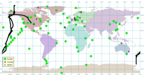
tive Global Air Sampling Network sites (Conway et al., 2011) and Environment Canada (EC) sampling sites. The 72 NOAA sites and six EC sites are shown in Fig. 2. The flask measurements are directly traceable to the World Meteorological Organization (WMO) CO2mole fraction scale (WMO X2007) (Zhao and Tans, 2006). Measurement accuracy determined from repeated analyses of CO2in standard gas cylinders using 25
ACPD
13, 26327–26388, 2013Inferring CO2 fluxes
from GOSATXCO2 F. Deng et al.
Title Page
Abstract Introduction
Conclusions References
Tables Figures
◭ ◮
◭ ◮
Back Close
Full Screen / Esc
Printer-friendly Version
Interactive Discussion
Discussion
P
a
per
|
D
iscussion
P
a
per
|
Discussion
P
a
per
|
Discuss
ion
P
a
per
|
Therefore, the accuracy and precision of flask measurements are undoubtedly high. When the observations are compared with the modeled observations, the model-data mismatches for the observations are larger, since representativeness errors must be accounted for.
The uncertainties assigned to these data for inverse modeling are calculated using 5
the statistics of the differences between the observations and the model simulations of the observations using the a priori emissions (Palmer et al., 2003; Heald et al., 2005). We calculated these uncertainties following the procedures detailed by Nassar et al. (2011), and these values are further scaled down to 68 % as the uncertainties used in our inverse modeling.
10
2.1.3 TCCON observations
We useXCO2 data from TCCON observatories to evaluate our inferred CO2 surface fluxes by examining whether the a posteriori CO2 distribution is in better agreement with the TCCON data. The TCCON sites use ground-based Fourier transform spec-trometers to measure high resolution spectra (0.02 cm−1) in the near infrared (3800– 15
15 500 cm−1), from whichXCO2is retrieved. A profile scaling retrieval approach is used to calculate the column CO2abundance. The column-averaged dry air mole fraction is then is computed as (Wunch et al., 2011)
XCO2=0.2095·CO col 2
Ocol2 , (4)
where O2col is the simultaneously retrieved atmospheric oxygen column density, and 20
ACPD
13, 26327–26388, 2013Inferring CO2 fluxes
from GOSATXCO2 F. Deng et al.
Title Page
Abstract Introduction
Conclusions References
Tables Figures
◭ ◮
◭ ◮
Back Close
Full Screen / Esc
Printer-friendly Version
Interactive Discussion
Discussion
P
a
per
|
D
iscussion
P
a
per
|
Discussion
P
a
per
|
Discuss
ion
P
a
per
|
precision and accuracy in the calibrated XCO2 data are both 0.8 ppm (2σ) (Wunch et al., 2010).
2.1.4 HIPPO aircraft measurements
The HIAPER Pole-to-Pole Observations (HIPPO) project is a sequence of five global aircraft measurement campaigns that sample the atmosphere from near the North Pole 5
to the coastal waters of Antarctica, from the surface to 14 km (Wofsy et al., 2011). The NCAR/NSF High-performance Instrumented Airborne Platform for Environmental Re-search (HIAPER), a modified Gulfstream V (GV) jet hosted the HIPPO campaigns. Major GHGs (CO2, CH4, N2O) and other important trace species were measured at high frequency, with two (or more) independent measurements for each to provide re-10
dundancy, check calibration and assess sensor drift. We use the CO2 field based on one-second data averaged to 10 s, from two (harmonized) sensors: CO2-QCLS and CO2-OMS. UTC (time), GGLAT (latitude from GPS), GGLON (longitude from GPS), and PSXC (static pressure) are the fields that we used to match observation with mod-eled CO2mixing ratio. In Sect. 3.2.2, we compare our results with data observed from 15
campaign 3 (HIPPO-3) in March and April 2010, and the route of the campaign is shown in Fig. 2.
2.1.5 Eddy covariance-based observations
We compare to land-atmosphere CO2fluxes from a so-called “upscaled” eddy covari-ance global product (MPI-BGC: Jung et al., 2009; Jung et al., 2011). This product de-20
rives a globally-gridded, time varying dataset from in situ measurements of net ecosys-tem exchange (NEE) at hundreds of flux tower sites worldwide. The towers’ instruments (sonic anemometer, infrared gas analyzer) measure fluxes on the order of 1 km, in ad-dition to ancillary measurements (e.g., meteorology) and other fluxes (Baldocchi et al., 2001; Baldocchi, 2008). The MPI-BGC product is derived from a suite of statistical 25
precipita-ACPD
13, 26327–26388, 2013Inferring CO2 fluxes
from GOSATXCO2 F. Deng et al.
Title Page
Abstract Introduction
Conclusions References
Tables Figures
◭ ◮
◭ ◮
Back Close
Full Screen / Esc
Printer-friendly Version
Interactive Discussion
Discussion
P
a
per
|
D
iscussion
P
a
per
|
Discussion
P
a
per
|
Discuss
ion
P
a
per
|
tion, and fraction of absorbed photosynthetically active radiation) available at the global scale to the NEE fluxes, and also derives Gross Primary Production (GPP) and Total Ecosystem Respiration (TER) products. The MPI-BGC product can be used only for specific analyses as the world is treated somewhat unrepresentatively like a flux site, e.g., undisturbed, growing, flat, biased towards temperate regions; the mean annual 5
flux, for instance, is not appropriate to compare to. Nonetheless, the MPI-BGC product is valuable for assessing relative spatial distributions, seasonal variability, and timing of min/max uptake, amplitude of the max-min uptake, interannual variability, and hotspots.
2.2 Forward modeling
The GEOS-Chem model (http://geos-chem.org) is used to simulate global atmospheric 10
CO2. The model is a global 3-D chemical transport model driven by assimilated me-teorology from the Goddard Earth Observing System (GEOS-5) of the NASA Global Modeling and Assimilation Office (GMAO). Nassar et al. (2010) described the recent update of the atmospheric CO2 simulation in GEOS-Chem. In this study, we employ the model at a horizontal resolution of 4◦×5◦, with 47 vertical layers. Our model sim-15
ulations include CO2 fluxes from fossil fuel combustion and cement production, from ocean surface exchange, from terrestrial biosphere assimilation and respiration, and from biomass burning. Specifically, these include (i) monthly national fossil fuel and ce-ment manufacture CO2emission from the Carbon Dioxide Information Analysis Center (CDIAC) (Andres et al., 2011); (ii) monthly shipping emissions of CO2from the Interna-20
tional Comprehensive Ocean–Atmosphere Data Set (ICOADS) (Corbett and Koehler, 2003; Corbett, 2004; Endresen et al., 2004, 2007); (iii) 3-D aviation CO2 emissions (Kim et al., 2007; Wilkerson et al., 2010; Friedl, 1997); (iv) monthly mean biomass burning CO2emissions from the Global Emissions Fire Database version 3 (GFEDv3) (van der Werf et al., 2010); (v) biofuel (heating/cooking) CO2 emission estimated by 25
ACPD
13, 26327–26388, 2013Inferring CO2 fluxes
from GOSATXCO2 F. Deng et al.
Title Page
Abstract Introduction
Conclusions References
Tables Figures
◭ ◮
◭ ◮
Back Close
Full Screen / Esc
Printer-friendly Version
Interactive Discussion
Discussion
P
a
per
|
D
iscussion
P
a
per
|
Discussion
P
a
per
|
Discuss
ion
P
a
per
|
Productivity Simulator (BEPS) (Chen et al., 1999), which was driven by NCEP reanal-ysis data (Kalnay et al., 1996) and remotely sensed leaf area index (LAI) (Deng et al., 2006). The annual terrestrial ecosystem exchange imposed in each grid box is neutral (Deng and Chen, 2011). The emission inventories for 2010 used in our GEOS-Chem simulation are summarized in Table 1.
5
2.3 Inverse problem and optimizing method
In the inversion analysis, the surface CO2 sources and sinks (x) are related to the atmospheric observations (y) by the following relationship
y=H(x)+ε, (5)
whereH is the forward atmospheric model (such as GEOS-Chem) and ε is the ob-10
servation error, or model-data mismatch, which reflects the difference between the observations and the modelled results, including errors associated with observations (instrument errors) and model errors. Considering an a priori estimate of the CO2flux
xa, we can construct a cost function
J(x)=1
2(H(x)−y)
T
S−o1(H(x)−y)+1
2(x−xa)
T
S−a1(x−xa), (6)
15
whereyis a the vector of observations andSoandSaare the observational and a priori error covariance matrixes, respectively. Minimization of the cost function, subject to the a priori constraint, provides an optimal estimate of the fluxes, based on the available observations.
In the version of GEOS-Chem employed here, we use a 4-dimensional variational 20
(4D-var) data assimilation system in which we optimize a set of scaling factors to adjust the fluxes in each model grid box to better reproduce the observations over a given time period. The 4D-var cost function that we minimize is given by
J(c)=1 2
N X
i=1
(fi(c)−yi)TS0,−1i(fi(c)−yi)+1
2(c−ca)
T
Sca−1
ACPD
13, 26327–26388, 2013Inferring CO2 fluxes
from GOSATXCO2 F. Deng et al.
Title Page
Abstract Introduction
Conclusions References
Tables Figures
◭ ◮
◭ ◮
Back Close
Full Screen / Esc
Printer-friendly Version
Interactive Discussion
Discussion
P
a
per
|
D
iscussion
P
a
per
|
Discussion
P
a
per
|
Discuss
ion
P
a
per
|
where N is the number of observations, yi, distributed in time over the assimilation window,cis the state vector of scaling factors, andcais the vector of a priori scaling factors, which we typically assume are unity. The a posteriori flux estimate for thejth grid cell is thus given byxj =c
jxa,j. Here the forward modelf includes the observation
operator that maps the modeled CO2profile to the GOSATXCO2observation space 5
XCOm2 =f(x)=XCO 2a+
X
j
hjaCO2,j(H(x)−ya)j, (8)
which is analogous to Eq. (3), with the modeled CO2 profile H(x) interpolated onto the GOSAT retrieval levels. Here XCO2m is the modelledXCO2, aCO2 is the GOSAT column averaging kernel, andhis the pressure weighting function provided with each GOSATXCO2retrieval.
10
The cost function is minimized iteratively using the L-BFGS algorithm (Liu and No-cedal, 1989) together with the adjoint of GEOS-Chem (Henze et al., 2007). The adjoint provides an efficient way to compute the sensitivity of the model output to inputs and model parameters, and was originally developed and used to optimize aerosol and CO sources (Henze et al., 2007, 2009; Kopacz et al., 2009, 2011; Jiang et al., 2011). In 15
this work, we apply the adjoint to optimize global surface CO2sinks and sources. In constructing the observational error covarianceS0, we used theXCO2error esti-mates provided with the ACOS-GOSAT dataset. However, these errors were uniformly inflated to ensure that the a posteriori reduced χ2=1 constraint (Tarantola, 2004) was approximately satisfied. This scaling is justified since the observation errors (or 20
the model-data mismatches) incorporate errors associated with observations and the model, which is difficult to characterize. For inversion of the XCO2_A, XCO2_B, and XCO2_C datasets, we inflated the reported ACOSXCO2errors by 1.7, 1.57 and 1.175, respectively.
The state vector in the inversion consists of the sum of CO2 fluxes from fossil fuel 25
ACPD
13, 26327–26388, 2013Inferring CO2 fluxes
from GOSATXCO2 F. Deng et al.
Title Page
Abstract Introduction
Conclusions References
Tables Figures
◭ ◮
◭ ◮
Back Close
Full Screen / Esc
Printer-friendly Version
Interactive Discussion
Discussion
P
a
per
|
D
iscussion
P
a
per
|
Discussion
P
a
per
|
Discuss
ion
P
a
per
|
covariance matrix, the a priori uncertainty estimates for these components ofSawere adjusted to ensure that the a posteriori reducedχ2=1 constraint was satisfied and to balance the observational term in the cost function. According to Marland et al. (2008), the uncertainty for estimates of global fossil fuel emissions is about 6 %. However, in constructing Sa, we assigned 16 % for the uncertainty of the fossil fuel emissions in 5
each month and each model grid box. For biomass burning, we started with an as-sumed uncertainty of 20 % that was then inflated to 38 % for emissions in each month and in each model grid box. The annual GPP estimate for 2010 is −119.5 Pg C and we assigned an uncertainty of 22 % of the GPP estimates in each 3 h time step and in each model grid. The TER, which is the sum of autotrophic and heterotrophic respi-10
ration, was specified to be 119.5 Pg C in 2010 since we assumed an annual balanced biosphere. We also assigned 22 % of the prior estimates in each 3 h time step and in each model grid as the prior TER uncertainty. For the ocean flux we assumed an a priori uncertainty of 44 %.
2.4 A posteriori uncertainty estimation
15
The optimization algorithm requires calculating the gradient of the cost function
∇J(c)=
N X
i=1
KTi S−10,i Kici−yi+(Sc
a)−1(c−ca), (9)
whereKi is the Jacobian associated with the linearization of the observation
opera-tor (forward atmospheric model) fi. The second derivative of the cost function is the
Hessian, 20
∇2J(c)=
N X
i=1
KTi S−10,iKi+ Sc a
−1
ACPD
13, 26327–26388, 2013Inferring CO2 fluxes
from GOSATXCO2 F. Deng et al.
Title Page
Abstract Introduction
Conclusions References
Tables Figures
◭ ◮
◭ ◮
Back Close
Full Screen / Esc
Printer-friendly Version
Interactive Discussion
Discussion
P
a
per
|
D
iscussion
P
a
per
|
Discussion
P
a
per
|
Discuss
ion
P
a
per
|
and for a linear system, such as CO2transport, the a posteriori error covariance matrix is given by the inverse of the Hessian,
ˆ
S=
N X
i=1
KTi S−0,1iKi+ Sca
−1 !−1
. (11)
We approximate the inverse of the Hessian using the Davidon–Fletcher–Powell (DFP) updating formula (Tarantola, 2004). This algorithm starts with an initial approximation 5
of the inverse of the Hessian and combines it with gradients information from recent iterations of the minimization algorithm to update ˆS. Since Eq. (7) optimizes the scaling factors but we need ˆSexpressed in the flux space, it is necessary to rescale Eq. (9) to express the gradient of the cost function with respect to changes in the fluxes, dJ/dx=
dJ/dc
dc/dx
, which yields 10
∇J(x)j=∇J(c)j/(x
a)j (12)
for the gradient of thejth flux element. With this transformation, the update to estimate a posteriori covariance proceeds as follows. Let
δxn=xn+
1−xn, (13)
δ∇J(x)n=∇J(x)
n+1− ∇J(x)n, (14)
15
and then the inverse of the Hessian can be approximated by DFP updating formula as
ˆ
Sn+1=Sˆn+
δxnδxTn
(δ∇J(x)n)Tδx n
−( ˆSnδ∇J(x)n)( ˆSnδ∇J(x)n)
T
(δ∇J(x)n)T( ˆS
nδ∇J(x)n)
, (15)
wherenis the iteration number. The approach used here to estimate the inverse Hes-sian is similar to that of Muller and Stavrakou (2005).
ACPD
13, 26327–26388, 2013Inferring CO2 fluxes
from GOSATXCO2 F. Deng et al.
Title Page
Abstract Introduction
Conclusions References
Tables Figures
◭ ◮
◭ ◮
Back Close
Full Screen / Esc
Printer-friendly Version
Interactive Discussion
Discussion
P
a
per
|
D
iscussion
P
a
per
|
Discussion
P
a
per
|
Discuss
ion
P
a
per
|
2.5 Initial condition and model run schemes
The initial fields of the atmospheric CO2 mixing ratio used are based on the results from an inversion analysis of flask observations from NOAA ESRL Carbon Cycle Co-operative Global Air Sampling Network sites and Environment Canada (EC) sampling sites. GEOS-Chem was run from 1996 to the end of 2007 without assimilation to obtain 5
a reasonable distribution of CO2in the troposphere and stratosphere, and then the flask observations were assimilated from January 2008 to the end of 2009. Comparison of the a posteriori CO2field in July 2009 with the GOSATXCO2revealed the assimilated CO2fields were biased high relative to the GOSAT v2.9 data. To obtain initial conditions for theXCO2inversions, we removed the global mean bias from the a posteriori CO2 10
distribution from the flask inversion (hereafter referred to as “the original initial field”) at 0 GMT on 1 July 2009. We scaled the original initial field by 0.99764, and 0.99734 to match the overall globalXCO2 values for XCO2_A, and XCO2_B, respectively, while we directly use the original initial field for XCO2_C. We carry out separate inversions for each of these GOSATXCO2datasets, which are referred to as RUN_A, RUN_B, and 15
RUN_C. For evaluation of the inversion results with independent surface data, we start with the original initial field, rather than the adjusted fields, to simulate the a posteriori atmospheric CO2. TheXCO2inversion analyses were conducted from 1 July 2009, to 31 December 2010, however, we report here only the results for 2010 to avoid possible discrepancies in the fluxes due to spin-up during the first 6 months.
20
3 Results
3.1 Optimized carbon fluxes and their uncertainties
ACPD
13, 26327–26388, 2013Inferring CO2 fluxes
from GOSATXCO2 F. Deng et al.
Title Page
Abstract Introduction
Conclusions References
Tables Figures
◭ ◮
◭ ◮
Back Close
Full Screen / Esc
Printer-friendly Version
Interactive Discussion
Discussion
P
a
per
|
D
iscussion
P
a
per
|
Discussion
P
a
per
|
Discuss
ion
P
a
per
|
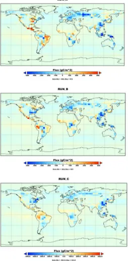
separately, we only report the net ecosystem exchange since the inferred GPP and TER fluxes will be highly correlated. Shown in Fig. 3 are annual fluxes for 2010 in-ferred from the GOSAT-ACOSXCO2 data with the three different screening and cor-rection schemes discussed in Sect. 2.1.1. The global total surface fluxes estimated from the three inversion analyses are similar:−3.79 PgC, −4.02 PgC, and−4.35 Pg C 5
for RUN_A, RUN_B, and RUN_C, respectively. Considering the 2.41±0.06 ppm an-nual mean global carbon dioxide growth rate for 2010 (Conway and Tans, 2012) and the 8.90 Pg C a priori carbon emission from fossil fuel burning (including na-tional fuel combustion and cement manufacturing (8.542 Pg C), internana-tional ship-ping (0.192 Pg C), and aviation (0.162 Pg C)) used for 2010, the global total surface 10
flux should be −3.78±0.13 Pg C (−3.65∼ −3.91 Pg C), using the conversion factor of 2.124 Pg C ppm−1to convert atmospheric CO2mixing ratio to Pg C. The estimate from RUN_A is in this range, whereas the estimates from RUN_B and RUN_C exceed the lower bound with greater surface carbon uptake of 0.11, and 0.44 Pg C. In terms of the land and ocean breakdown, we estimate that 2.16–2.77 Pg C is fixed by the terrestrial 15
biosphere, and 1.49–1.63 Pg C is absorbed by the ocean in 2010, based on the three inversions. The estimates for the oceanic uptake vary less between the three inver-sions, which may be due to the fact that the oceanic flux estimates are dominated by the Takahashi et al. (2009) a priori fluxes because we did not use any atmospheric CO2observations over the ocean in the three inversions.
20
As can be seen in Fig. 3, the differences in the spatial distribution of the terrestrial carbon fluxes are large. Significant differences can be found between the inferred CO
2 fluxes from RUN_A and RUN_B, and between those from RUN_A and RUN_C, while the distribution obtained from RUN_B is relatively similar to that obtained from RUN_C. There are large differences, for example, over North America and South America (see 25
ACPD
13, 26327–26388, 2013Inferring CO2 fluxes
from GOSATXCO2 F. Deng et al.
Title Page
Abstract Introduction
Conclusions References
Tables Figures
◭ ◮
◭ ◮
Back Close
Full Screen / Esc
Printer-friendly Version
Interactive Discussion
Discussion
P
a
per
|
D
iscussion
P
a
per
|
Discussion
P
a
per
|
Discuss
ion
P
a
per
|
becomes much weaker when we use XCO2_B, and XCO2_C datasets. Although there are no grid boxes that are strong sources of CO2 in RUN_C, the annual CO2 source for tropical South America inferred from XCO2_C data is significantly greater than that inferred from XCO2_A, and XCO2_B data, as the number of inferred source grid cells is much greater in RUN_A than in RUN_B.
5
To help interpret our results, the monthly land fluxes are aggregated into the 11 TransCom land regions (Gurney et al., 2002) that are widely used. The total annual flux and the seasonal variations of the fluxes for each region are shown in Figs. 4 and 5, respectively. We estimate a sink for all four Eurasian regions (Europe, Boreal Eurasia, Temperate Eurasia, and Tropical Asia), as shown in Fig. 4, in all three inver-10
sion analyses. The estimated aggregated uptake for these regions is 3.69, 2.94, and 2.55 Pg C from RUN_A, RUN_B and RUN_C, respectively. In the extratropics, the esti-mated fluxes are most similar across the threeXCO2inversions for Boreal Eurasia and Temperate Eurasia, for which we estimated an annual CO2 uptake in range of 0.49 to 0.68 Pg C and 0.51 to 0.64 Pg C, respectively. Their seasonal variations (Fig. 5) are also 15
similar in the three inversions. We note that the a posteriori fluxes in Boreal Eurasia are close to the a priori used, reflecting, as discussed below, the lack of observational cov-erage in winter and with observations over the boreal region only available during May through September.
For Tropical Asia, the threeXCO2 inversions suggested a sink in the range of 0.69 20
to1.32 Pg C. The differences between inversions are manifested mainly in the region around the Indonesian islands (see Fig. 3), and between May to September (see Fig. 5). These differences amount to an increased uptake of about 0.63 Pg C in the annual regional carbon budget (Fig. 4) in RUN_A compared to RUN_C.
The largest differences in the inferred fluxes for the threeXCO
2inversions were ob-25
ACPD
13, 26327–26388, 2013Inferring CO2 fluxes
from GOSATXCO2 F. Deng et al.
Title Page
Abstract Introduction
Conclusions References
Tables Figures
◭ ◮
◭ ◮
Back Close
Full Screen / Esc
Printer-friendly Version
Interactive Discussion
Discussion
P
a
per
|
D
iscussion
P
a
per
|
Discussion
P
a
per
|
Discuss
ion
P
a
per
|
for Boreal North America also varied significantly between the three inversions, but the absolute magnitude of the differences was small. We also conducted an inversion analysis of the surface flask data and the differences between the fluxes inferred from the flask data and those based on theXCO2for Temperate North American is striking. With XCO2_A we estimated a source of about 0.5 Pg C for Temperate North America, 5
whereas with the flask data we estimated a sink of about 0.7 Pg C (Fig. 4). Examination of the seasonal variations in Fig. 5 shows that there are significant differences among the three inversions in the timing and extent of the uptake of CO2 in July, August, and September in Boreal North America. In Temperate North America the monthly mean uptake in RUN_A is systematically smaller from May through September than in the 10
other two runs. In Temperate South America, CO2 uptake during the growing season in RUN_A is much less than in the other two runs, especially between January–April. Considering the spatial distribution, these differences in Temperate South America are mostly caused by the stronger uptake in RUN_C and RUN_B than in RUN_A in the eastern part of this region.
15
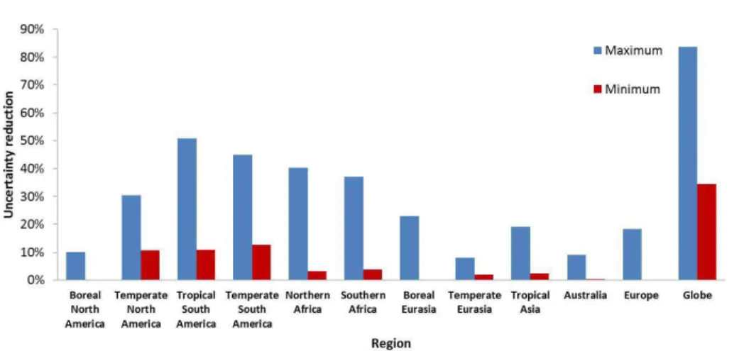
The posterior errors derived from the 4D-Var inversion using Eq. (15) have been aggregated to the TransCom regions. The uncertainties of the land fluxes and the flux for each month are given in Fig. 5. These uncertainties can be further used to calculate the uncertainty reduction percentage (Deng et al., 2007), given as
Ur=
1− σ σa
×100 %. (16)
20
whereσandσaare the a posteriori and a priori uncertainties, respectively. The uncer-tainty reduction obtained for RUN_A is shown in Fig. 6. The unceruncer-tainty reduction on the regional flux estimates varies significantly from region to region. The minimum uncer-tainty reductions can be as small as less than 1 % for the three northern high-latitude regions (Boreal North America, Europe, and Boreal Eurasia) during winter months, 25
ACPD
13, 26327–26388, 2013Inferring CO2 fluxes
from GOSATXCO2 F. Deng et al.
Title Page
Abstract Introduction
Conclusions References
Tables Figures
◭ ◮
◭ ◮
Back Close
Full Screen / Esc
Printer-friendly Version
Interactive Discussion
Discussion
P
a
per
|
D
iscussion
P
a
per
|
Discussion
P
a
per
|
Discuss
ion
P
a
per
|
flux estimates was obtained for the fluxes inferred for Temperate North America, the two South American regions, and the two African regions. The largest uncertainty re-duction that we obtained was about 50 % for Tropical South America. We note that these estimates of uncertainty reduction depend largely on our assumed a priori un-certainty. Comparison of the monthly mean fluxes in Fig. 5 indicates the differences 5
in the flux estimates inferred from the different datasets is larger than the estimated a posteriori uncertainties, suggesting that it is likely that we have underestimated the observation errors. Neglect of spatial and temporal correlations in the a priori error co-variance matrix would also result in an underestimate of the a posteriori errors and, consequently, an overestimate of the uncertainty reduction. Clearly, the estimated un-10
certainty reduction depends strongly on the specification of the observation and a priori error covariance matrix, which are difficult to characterize. Therefore, in our interpre-tation of the uncertainty reduction in Sect. 4 we will focus on the relative uncertainty reduction between the different regions and not on the magnitude of the error reduction.
3.2 Evaluation of the inversions
15
3.2.1 Comparison with GOSATXCO2
The objective of the inversion analysis, as described by Eq. (7), is to optimize the fluxes to minimize the mismatch between the model and observations. One way of assessing the success of the inversion is by the degree to which the a posteriori CO2 matches the observations. Shown in Fig. 7 are the model and GOSAT XCO2 differences for 20
RUN_A. It shows that the distribution of the model and observations differences is approximately Gaussian. As an indication of the overall inversion performance, the mean global bias is reduced from 2.72 ppm to 0.04 ppm, while the 1σ spread is also reduced from 2.18 ppm to 1.65 ppm. On the hemispheric scale, the residual bias is smaller in the Northern Hemisphere (NH) than in the Southern Hemisphere (SH). In the 25
ACPD
13, 26327–26388, 2013Inferring CO2 fluxes
from GOSATXCO2 F. Deng et al.
Title Page
Abstract Introduction
Conclusions References
Tables Figures
◭ ◮
◭ ◮
Back Close
Full Screen / Esc
Printer-friendly Version
Interactive Discussion
Discussion
P
a
per
|
D
iscussion
P
a
per
|
Discussion
P
a
per
|
Discuss
ion
P
a
per
|
bias is 0.08 ppm (reduced from 2.02 ppm, with a decrease in the standard deviation from 1.88 ppm to 1.39 ppm). While the mean biases have been reduced satisfactorily in both hemispheres, the larger standard deviation obtained in the NH may reflect the difficulty of reliably capturing the greater biospheric sources and sinks in the NH.
We also examined the seasonality of the residual bias, focusing on April–September 5
as the growing season and October–March as the non-growing season in the NH, and vice versa for the SH, to broadly reflect the hemispheric biosphere carbon cycle dy-namics. During the growing season, the residual biases were 0.00 ppm and 0.03 ppm for the NH and SH, respectively. During the non-growing season, the biases were 0.02 and 0.09 ppm, for the NH and SH, respectively. We believe that the relatively small bi-10
ases of 0.03 ppm and 0.00 ppm obtained for the SH and NH, respectively, during their growing season is due to the fact that moreXCO2data are available to constrain the inversion analysis during these periods. One common feature among the four cases examined is that the standard deviations of the a posteriori biases are greater during the growing season on both hemispheres than during the non-growing season, indicat-15
ing that larger uncertainties may be related to simulating the summertime drawdown of atmospheric CO2.
3.2.2 Comparison with independent observations
Flask observations
Flask observations provide the research community with highly accurate and precise 20
atmospheric CO2measurements that are often used to calibrate new atmospheric CO2 measurements. We use here flask observations from the 78 observing sites shown in Fig. 2, corresponding to 3016 flask observations in 2010, to evaluate the a posteriori CO2fluxes. We sampled the modeled CO2distribution at the appropriate measurement location and time (to within one hour of the measurement time). Using the a posteriori 25
ACPD
13, 26327–26388, 2013Inferring CO2 fluxes
from GOSATXCO2 F. Deng et al.
Title Page
Abstract Introduction
Conclusions References
Tables Figures
◭ ◮
◭ ◮
Back Close
Full Screen / Esc
Printer-friendly Version
Interactive Discussion
Discussion
P
a
per
|
D
iscussion
P
a
per
|
Discussion
P
a
per
|
Discuss
ion
P
a
per
|
These mean differences for RUN_A and RUN_B could be due to the overall systematic errors transferred from theXCO2data when we adjusted the initial CO2distribution in the inversion to remove the mean mismatch with the GOSAT data. Therefore, it would be inappropriate to directly compare the modeled a posteriori mixing ratios against real flask observations to evaluate our flux estimates. Instead we simulated the a posteriori 5
CO2mixing ratios, based on the optimal CO2flux estimates, starting from the original initial CO2 field (which as discussed in Sect. 2.5, was based on an assimilation of the surface data).
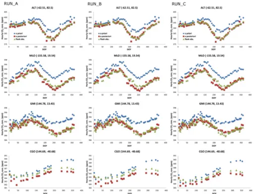
Figure 8 shows the observed and simulated CO2time series at four flask sites: ALT (Alert, Nunavut, Canada), MLO (Mauna Loa, Hawaii, USA), GMI (Mariana Islands, 10
Guam), and CGO (Cape Grim, Tasmania, Australia). Because we assumed a balanced biosphere (with zero annual net uptake) for our a priori fluxes, the a priori CO2 distribu-tion significantly overestimates the observadistribu-tions at the flask sites by the end of 2010. The a priori overestimate largely reflects the well-established secular increase in atmo-spheric CO2 due to anthropogenic emissions, and the inversion successfully corrects 15
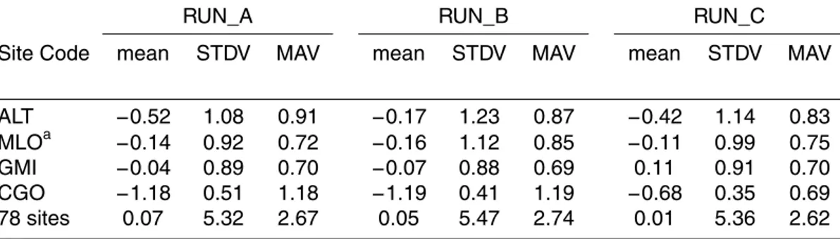
for it. In general, the seasonal variation of the observed atmospheric CO2time series has been satisfactorily simulated using the a posteriori fluxes, optimized from ACOS GOSATXCO2 data, considering the spatial and temporal resolution of the model. We intentionally started with a poor a priori flux to better assess the ability of the obser-vations to constrain the flux estimates. The mean, the standard deviation (STDV), and 20
the mean absolute value (MAV) of the mismatch between the a posteriori model and observations are listed in Table 2. For ALT, MLO, and GMI, the mean differences are small, much less than 1 ppm. For CGO, however, the a posteriori CO2 is biased low by slightly more than 1 ppm for RUN_A and RUN_B, while the bias was significantly reduced to−0.68 for RUN_C. For all 78 flask sites, the mean of the model-observation 25
ACPD
13, 26327–26388, 2013Inferring CO2 fluxes
from GOSATXCO2 F. Deng et al.
Title Page
Abstract Introduction
Conclusions References
Tables Figures
◭ ◮
◭ ◮
Back Close
Full Screen / Esc
Printer-friendly Version
Interactive Discussion
Discussion
P
a
per
|
D
iscussion
P
a
per
|
Discussion
P
a
per
|
Discuss
ion
P
a
per
|
extratropics. However, the magnitude of the underestimate is highly variable. At Palmer Station, Antarctica (PSA), for example, the mean difference is only−0.21 ppm and the MAV is 0.21 (not shown) in RUN_A, compared to−1.18 ppm for the mean difference and 1.18 for the MAV at CGO. Examination of the mean and MAV suggests that RUN_C provides a relatively better overall simulation compared with observations from all 78 5
sites.
TCCON observations
We evaluated the a posteriori flux estimates using TCCON by comparing the obser-vations with the a posteriori atmospheric CO2 mixing ratios that were produced with the model simulation initialized with the original initial CO2field. As with the flask data, 10
the model was sampled at the observation location and time (to within one hour). To compare with the TCCONXCO2, the modelled CO2concentrations are mapped to the TCCON 71 vertical layers and then transformed using the a priori profile and average kernel extracted from the TCCON dataset. Finally, theXCO2values are calculated us-ing the approach of Wunch et al. (2011). Figure 9 shows the observed and modeled 15
XCO2time series at four selected sites: (1) Lamont, USA, (2) Sodankylä, Finland, (3) Izana, Tenerife, and (4) Wollongong, Australia. The a posteriori CO2 field reproduced well the observed seasonal variations at these four sites. However, the model under-estimated theXCO2 at Lamont and Izana in summer (between days 150–250), and overestimated it at Sodankylä and Wollongong throughout 2010. Using the scaled ini-20
tial field, our calculation shows that the means of the mismatches between the modeled a posteriori hourly atmospheric CO2 mixing ratios and the observations at 13 TCCON sites in 2010 are−0.79 ppm,−1.27 ppm, and 0.06 ppm for all three inversions, respec-tively.
The mean model and observation mismatch, the standard deviation (STDV), and the 25
ACPD
13, 26327–26388, 2013Inferring CO2 fluxes
from GOSATXCO2 F. Deng et al.
Title Page
Abstract Introduction
Conclusions References
Tables Figures
◭ ◮
◭ ◮
Back Close
Full Screen / Esc
Printer-friendly Version
Interactive Discussion
Discussion
P
a
per
|
D
iscussion
P
a
per
|
Discussion
P
a
per
|
Discuss
ion
P
a
per
|
XCO2at Park Falls, Orleans, Karlsruhe, Bialystok, Darwin, and Lauder are well simu-lated by the a posteriori fluxes from all three inversions, with mean biases that are less than or equal to 0.70 ppm. RUN_B produced the best a posteriori CO2 compared to the TCCON observations in Southern Hemisphere (including Darwin, Wollongong, and Lauder) in terms of both the mean and the MAV, while RUN_A produced the best a pos-5
teriori CO2comparing with northern subtropical (Lamont, and Izana) observations. For the northern sites, no single inversion consistently agrees well with all the observations, however, RUN_B and RUN_C generally produced better a posteriori CO2 fields rela-tive to the observations. Considering all 13 sites, RUN_C has the least absolute mean bias (0.06 ppm) and the least MAV (0.91 ppm). It also has the strongest correlation 10
(r2=0.80) with the observedXCO
2at all 13 sites.
HIPPO aircraft measurements
As discussed in Sect. 2.1.4, we compare our a posteriori CO2 fields with the 10 s averaged HIPPO-3 data. At this temporal resolution, the HIPPO data will reflect CO2 on spatial scales smaller than the model resolution. We do not average the HIPPO data 15
onto the model grid, so the differences between the model and the observations will also reflect representativeness errors associated with the coarse model grid. Listed in Table 4 are the mean differences, the standard deviation, and the mean absolute value of model and observation mismatch for all 24 303 HIPPO-3 observations. In general, the results from the three inversions are not significantly different from each other. 20
We estimated mean differences of−0.07 ppm,−0.08 ppm, and−0.17 ppm for RUN_A, RUN_B, and RUN_C, respectively. In contrast, using the scaled initial field results in mean differences between the a posteriori CO
2 and the HIPPO data of −1.01 ppm, −1.12 ppm, and −0.17 ppm, respectively, reflecting the global mean bias in the initial conditions used for theXCO2inversions.
25
ACPD
13, 26327–26388, 2013Inferring CO2 fluxes
from GOSATXCO2 F. Deng et al.
Title Page
Abstract Introduction
Conclusions References
Tables Figures
◭ ◮
◭ ◮
Back Close
Full Screen / Esc
Printer-friendly Version
Interactive Discussion
Discussion
P
a
per
|
D
iscussion
P
a
per
|
Discussion
P
a
per
|
Discuss
ion
P
a
per
|
optimal surface fluxes from our three inversions with the HIPPO-3 observations. As our model is sampled with a temporal resolution of one hour, and the spatial resolution of the model is coarse (4◦×5◦), the modeled CO2 does not reproduce much of the detailed structure seen in the observations. The a posteriori simulations based on the optimal fluxes from RUN_B deviate from the observation the most in the southern high-5
latitudes. For example, the mean differences in the southern high latitudes, 70◦S–45◦S can be as large as−0.92 ppm. However, the simulations based on a posteriori fluxes from RUN_B are less biased relative to the observations in the tropics and the Northern Hemisphere. The a posteriori simulation based on RUN_C has the smallest bias in the Southern Hemisphere between 15◦S to 70◦S, but the largest bias in the tropics (15◦S 10
to 15◦N). The posterior CO2 from RUN_A deviate from the observations the most in the Northern Hemisphere (15◦N to 80◦N). Overall, the simulations compare well to the HIPPO data. The correlation between the a posteriori simulations and the observations arer2=0.96 for all three inversion runs.
Eddy covariance-derived product
15
In Fig. 11 we compare our inferred fluxes for Temperate North America and Europe with the MPI-BGC fluxes (Jung et al., 2011), which are empirically derived from eddy covariance measurements. We focus on North America and Europe for this compari-son since the density of eddy covariance towers is greatest in these regions. For Tem-perate North America, the MPI-BGC fluxes suggest weaker uptake in May and June 20
than inferred from RUN_B, whereas the June MPI-BGC flux is in agreement with the estimates in RUN_A and RUN_C. However, for July – September the MPI-BGC data product suggests greater uptake than the threeXCO2 inversions and the flask inver-sion. For Europe, the MPI-BGC data are generally consistent with the results of the inversions. The major discrepancy between the threeXCO2 inversions and the MPI-25
ACPD
13, 26327–26388, 2013Inferring CO2 fluxes
from GOSATXCO2 F. Deng et al.
Title Page
Abstract Introduction
Conclusions References
Tables Figures
◭ ◮
◭ ◮
Back Close
Full Screen / Esc
Printer-friendly Version
Interactive Discussion
Discussion
P
a
per
|
D
iscussion
P
a
per
|
Discussion
P
a
per
|
Discuss
ion
P
a
per
|
4 Discussion
4.1 Regional flux estimates
Terrestrial ecosystem (biosphere) models often underestimate the seasonal amplitude of CO2 in the Northern Hemisphere (Randerson et al., 2009), and inversion analyses that employ these terrestrial ecosystem models to provide a priori flux estimates un-5
derestimate the CO2seasonal amplitude by 1 to 2 ppm (Basu et al., 2011; Peters et al., 2010). In this study, we used the annual balanced, 3 hourly terrestrial ecosystem fluxes as described by Deng and Chen (2011), which also produced a weak seasonal cycle in the a priori CO2fields. However, as shown in Figs. 8 and 9, the a posteriori simula-tions reproduced well the amplitude of the seasonal cycle measured at the flask and 10
TCCON sites. This improvement in the modeled seasonal cycle could be attributed to the good spatial coverage of the GOSAT observations during the growing season. This correction in the modeled seasonal cycle is reflected in the significantly greater uptake of CO2during the growing season obtained for the regions in the extratropical Northern Hemisphere (Fig. 5).
15
Using the ACOSXCO2data screened and bias corrected by the three different ap-proaches produced significantly different surface fluxes for regions such as Boreal North America, Temperate North America, and Temperate South America. The sen-sitivity of the inferred flux estimates for Boreal North America is not surprising since the GOSAT observational coverage is limited at high latitudes over North America. 20
The Temperate North America region has been described as a sink in previous in-versions using flask observations of atmosphere CO2(Deng and Chen, 2011; Gurney et al., 2004; Peters et al., 2007; Rayner et al., 2008; Deng et al., 2007). Here we esti-mated the region to be a significant source in RUN_A, but a weak sink in RUN_B and a strong sink in RUN_C. Our flask inversion suggested a stronger sink for the region. 25
ACPD
13, 26327–26388, 2013Inferring CO2 fluxes
from GOSATXCO2 F. Deng et al.
Title Page
Abstract Introduction
Conclusions References
Tables Figures
◭ ◮
◭ ◮
Back Close
Full Screen / Esc
Printer-friendly Version
Interactive Discussion
Discussion
P
a
per
|
D
iscussion
P
a
per
|
Discussion
P
a
per
|
Discuss
ion
P
a
per
|
the June uptake. In contrast, in RUN_B and RUN_C, we estimated stronger uptake in June. Unlike the flask inversion, all theXCO2inversions produced much weaker uptake in July compared to June. Comparison with the TCCON observations at Lamont from day 120–250 (Fig. 9) shows the strong negative bias for RUN_B and RUN_C, which could indicate that the stronger uptake inferred in these inversions for Temperate North 5
America represent an overestimate of the actual sink during the growing season (in the absence of compensatory changes in the flux from other regions). Surface flask obser-vations, for example, at the KEY site and inland at NWR and SGP (not shown), also suggest that the summertime sinks estimated in RUN_B and RUN_C for Temperate North America were overestimated. A weak sink for Temperate North America is pos-10
sible for 2010 as a result of the cold spring and hot and dry summer in the southeast US during 2010 (Blunden et al., 2011). In addition, fire emissions in British Columbia, Canada, in July would have further reduced the net uptake of CO2 from Temperate North America in 2010. Indeed, these could be responsible for the strong decrease in uptake in the threeXCO2inversions in July.
15
For Temperate South America, we estimated a strong source in RUN_A, a weak source in RUN_B, and a strong sink in RUN_C (Fig. 4). As shown in Fig. 5, these differences are largely due to the estimated uptake during January to May. For these months, RUN_B and RUN_C suggest greater uptake than RUN_A, with sink estimates comparable to those inferred from the flask data and similar to the a priori fluxes. Com-20
parison with the flask data from the PSA flask station at the South Pole (not shown), reveals that the a posteriori CO2concentrations from all threeXCO2inversions under-estimate the observed CO2 concentrations, with the underestimate being greater for RUN_B during the first half of 2010. However, this is not the case for RUN_C though the inferred fluxes from XCO2_C are almost identical to those from XCO2_B for the same 25