School of Economics and Management

Carlos Pestana Barros & Nicolas Peypoch

A Comparative Analysis of Productivity Change in Italian and Portuguese Airports

WP 006/2007/DE _________________________________________________________

António Afonso & João Tovar Jalles

Growth and Productivity: the role of Government Debt

WP 13/2011/DE/UECE _________________________________________________________

Department of Economics

W

P

ISSN Nº 0874-4548

School of Economics and Management

Growth and Productivity: the role of

Government Debt

António Afonso

and João Tovar Jalles

2011

Abstract

We use a panel of 155 countries to assess the links between growth, productivity and government debt. Via growth equations we assess simultaneity, endogeneity, cross-section dependence, nonlinearities, and threshold effects. We find a negative effect of the debt ratio. For the OECD, the higher the debt maturity the higher economic growth; financial crisis are

detrimental for growth; fiscal consolidation promotes growth; and higher debt ratios are

beneficial to TFP growth. The growth impact of a 10% increase in the debt ratio is -0.2% (0.1%) respectively for countries with debt ratios above (below) 90% (30%), and an endogenous debt ratio threshold of 59% can be derived.

JEL: C23, E62, H50.

Keywords: government debt, crises, panel analysis.

_____________________________ *

We are grateful to Giancarlo Corsetti for useful discussions at the beginning of the project, to participants in an ECB seminar for useful comments. The research was conducted while João Tovar Jalles was visiting the ECB whose hospitality was greatly appreciated. The opinions expressed herein are those of the authors and do not necessarily reflect those of the ECB or the Eurosystem.

$ _{ISEG/UTL - Technical University of Lisbon, Department of Economics; UECE – Research Unit on Complexity and}

Economics. UECE is supported by FCT (Fundação para a Ciência e a Tecnologia, Portugal), email: aafonso@iseg.utl.pt.

# _{European Central Bank, Directorate General Economics, Kaiserstraße 29, D-60311 Frankfurt am Main, Germany.}

email: antonio.afonso@ecb.europa.eu.

+ _{University of Cambridge, Faculty of Economics, Sidgwick Avenue, Cambridge CB3 9DD, United Kingdom, email:}

1. Introduction

The relevance of government debt for economic growth has become crucial,

particularly in a context where policy makers have to face increasing fiscal imbalances. In

terms of economic theory, at moderate levels of government debt, fiscal policy may induce

growth, with a typical Keynesian behaviour. However, at high debt levels, the expected

future tax increases will reduce the possible positive effects of government debt,

decreasing investment and consumption resulting in less employment and lower output

growth. Unfortunately, the empirical evidence that is currently available to shed light on

the importance of government debt (and related aspects) for growth of productivity is not

very conclusive. This paper attempts to fill some gaps and intends to provide some

additional empirical evidence of the effects of government debt (and its maturity structure)

on output growth and productivity for advanced countries (OECD) as well as emerging and

developing countries.

We have recently observed a revival in this theme fuelled by the substantial worsening

of public finances in many advanced (and other) economies as a result of the 2008/09

financial and economic crisis. In response, governments around the world implemented

important fiscal stimulus. More than ever it is important to understand the effects of

government debt on growth, capital accumulation and productivity, particularly when

associated with financial crisis.

The linkages between fiscal policy and growth have been the object of several analyses

For instance, Gemmell (2004) has summarised many existing empirical work dividing it

into three generation studies depending on the econometric methods used. Even though our

main purpose is empirical in nature, it is worth referring to some initial theoretical

contributions which serve as the underlying basis for our analysis. In particular, Modigliani

(1961) and Diamond (1965) first, and later Saint-Paul (1992), take a theoretical approach

based on a neoclassical growth model and suggest that an increase in public debt will

always decrease the growth rate of the economy. Regarding the developments of

government debt, Corsetti et al. (2010) discuss the importance of the reversal of significant

fiscal imbalances, to ensure the curbing of government debt, notably in a context where

monetary policy is limited by a zero lower bound regarding policy interest rates.

With respect to the empirical evidence, most papers have focussed on advanced

countries. Authors looking at mixed samples such as Schlarek (2004) focusing on a panel

of 59 developing and 24 advanced countries for the period 1970-2002 concludes that, for

growth. For advanced countries, he does not find any robust evidence, suggesting that

higher public debt levels are not necessarily associated with lower GDP growth rates.

Checherita and Rother (2010) look at the Euro-area from 1970 to 2010 and find a nonlinear

impact of debt on growth with a turning point at about 90-100% of GDP. On the same line,

Kumar and Woo (2010) used 38 advanced and emerging countries from 1970 to 2007 and

also find an inverse relationship between initial debt and subsequent growth, controlling

for other determinants of growth.

On the other hand, de la Fuente (1997) using OECD countries between 1965 and 1995

report evidence of a sizeable negative externality effect of government on the level of

productivity. In addition, Dar and Amirkhalkhali (2002) for a sample of 19 OECD

countries find that Total Factor Productivity (TFP) growth and productivity of capital are

weaker in countries with larger government (which can be proxied by the debt-to-GDP

ratio).

In this study we use cross-sectional/time series data for a panel of 155 developed and

developing countries for the period 1970-2008. We do not present or test a comprehensive

theory of economic growth. Rather, we are investigating the stability of coefficients over

time and across countries (and groups of homogeneous economies). In the empirical

estimation, the paper makes use of growth equations and growth accounting techniques (to

explore different channels of impact) and focus on a number of econometric issues that can

have an important bearing on the results. In particular, we assess such issues as

simultaneity, endogeneity, the relevance of nonlinearities, and the importance of outliers.

Therefore, this paper contributes to the literature by assessing the debt-growth nexus

with a diversified variety of methods, providing sensitivity and robustness, and, in more

specific terms, by addressing the following issues: i) The impact of government debt, and

its maturity, on growth, the existence of nonlinearities, and the relevance of debt

thresholds. ii) The relevance of financial development (e.g., banking sector development,

stock market development, for which we build several financial development proxies) and

the impact of financial crises (debt, currency and banking) on the debt-growth relationship.

iii) On a growth accounting perspective, the impact on TFP growth (for that purpose we

build a measure of TFP), capital stock accumulation, private and public investment. iv)

Differences between country groups (OECD vs. Emerging and Developing).

Our main results can be summarised as follows:

i) there is a negative effect of the government debt ratio for the full sample; ii) a quadratic

maturity the higher economic growth; iv) financial crisis are detrimental for growth,

notably with high debt ratios; v) fiscal consolidation promotes growth in a non-Keynesian

fashion; vi) for countries with debt ratios above (below) 90% (30%) the growth impact of a

10% increase in the debt ratio is -0.2.% (0.1%); vii) an endogenous debt ratio threshold of

59% can be derived for the full sample; viii) financial development, stock market

development, financial efficiency and bond market development positively affect growth

in the OECD; ix) higher debt ratios are beneficial to TFP growth, the growth of capital

stock per worker, and detrimental to the levels of private and public investment; x) the

higher the household’s debt burden coupled with higher government debt, the lower output

growth; xi) most results are confirmed even after we address cross-sectional dependence.

The paper is organised as follows. Section two describes the analytical and

econometric methodology. Section three presents the data, in particular the construction of

the TFP and financial development measures. Section four discusses our main results.

Section five concludes.

2. Methodology

2.1 Analytical framework

A neoclassical growth model provides the analytical framework for our analysis, and

the underlying basic aggregate production function can be written as Y=F(L,K), with Y

being the real aggregated output; L, labour force or population; K, capital (physical and

human). This model suggests that poor countries should have a high return to capital and a

fast growth in transition to the steady-state. However, there are several factors that could

interfere with this result. Therefore, the standard growth model is based on a conditional

convergence equation that relates real growth of per capita GDP to the initial level of

income per capita,1 investment-to-GDP ratio (a proxy for physical capital in a standard

neoclassical production function), a measure of human capital or educational attainment,

and the population growth rate, which is augmented to include the level of government

debt (as a share of GDP) – and some variants based on government debt maturity.2 This is

complemented with some controls, one of which is a measure of trade openness,3 as

_____________________________ 1

The initial level of income per capita is not only a robust and significant variable for growth (in terms of conditional or beta convergence), but output is generally correlated with fiscal variables, in particular, tax revenues and government expenditures.

2

The underlying model has its theoretical underpinnings from Landau’s (1983), Kormendi and Meguire’s (1985) or Ram’s (1986) formulations.

3

commonly found in the growth literature to expand the model beyond a closed-economy

form.

Ultimately, our aggregate production function is Y=F(L,K,D) with D being a

debt-related variable of interest. Specifically, D alternatively consists of the total government

debt ratio; short-term government debt ratio; long-term government debt ratio; short-term

government debt as a share of total government debt.The baseline specification assumes a

linear relationship between D and growth:

it i t it it j io

it it

it y y x D

y − ₋₁ =α +β₀ +β₁ +γ +η +ν +ε (1)

where yit −yit−1represents the growth rate of real GDP per capita; yi0is the initial value of

the real GDP per capita;4 xjit, j=1,2 is a vector of control variables; D_it is a debt-related

variable; η_t and ν_icorrespond to the country-specific fixed effect and time-fixed effect,

respectively, andε_it is some unobserved zero mean white noise-type column vector

satisfying the standard assumptions. α β β, ₀, ₁ and γ are unknown parameters to be

estimated.

The vector x1it (benchmark) comprises population growth, trade openness, gross fixed

capital formation (% GDP) and an education proxy for human capital corresponding to

Barro and Lee’s (2010) secondary school attainment (in Tables 1 to 4.b). x1it is enlarged

with the debt maturity variable as well as an interaction term (in Table 4.c). Table 5

includes as controls x1it and four interaction terms with financial crises-related dummies.

Table 6 uses alternatively x2itcomposed of the initial values of the variables included in

it

x1 (apart from population growth) together with the initial values (at the beginning of

each 5-year period) for inflation (CPI-based), initial government size (see Appendix 2),

initial financial depth (or liquid liabilities over GDP), banking crisis dummy and

government balance ratio. Table 7 includes x2it together with a number of interaction

terms with debt threshold levels and geographical dummies. Tables 11.a-b use x2it and

Table 12 x1it.

To capture a possible non-linear relationship, we also consider a quadratic term in (1).

Such specification would support, in this context, a so-called Laffer hypothesis if the

coefficient on debt is positive and the coefficient on debt squared is negative. Furthermore, integrated international financial markets may offer more scope to absorb shocks through risk sharing, suggesting there is less need for governments to step in. For instance, Afonso and Furceri (2008) find that such risk sharing is lower among the EU countries than in the US states.

4

we access the existence of other non-linear and threshold effects by making use of several

dummy (binary-type) variables and interaction terms in our regressions, as it will be

explained in the next section.

Finally, taking a growth accounting approach, we compute a measure of TFP and we

examine the influence of fiscal variables in affecting its growth rate, as well as the growth

rate of per worker capital stock, and private and public investment levels.

2.2. Econometric approaches

2.2.1. Panel techniques

The argument for cross-section studies over long time spans has been that less

interesting short- to medium-term effects, such as business cycle effects, are thereby

eliminated. However, a number of problems with cross-section studies using long time

spans need to be addressed. The most important of these may be a potentially severe

simultaneity problem. The cross-country regressions are usually based on average values

over long time periods. In such cases, e.g., the level of government spending is likely to be

influenced by demographics, in particular an increasing share of elderly. At the same time

the share of elderly is correlated with GDP. Thus, errors in the growth variable will affect

GDP, demographics and fiscal variables as a share of GDP, which are then correlated with

the error term in the growth regression.

A second problem is that cross-section studies using long observation periods give rise

to an endogenous selection of government spending (tax) policy. For example, countries

that raise taxes and experience lower growth during the observation period are more likely

to change the policy stance afterwards and, for instance, reduce taxes, such as Ireland did

during the 1980s.

A third related problem is that cross-section analysis may be inefficient since it

discards information on within-country variation. While both the simultaneity effect and

the use of within-country variation are arguments in favour of panel regressions with

shorter time spans, there are also risks. When the period of observation is short, it is less

likely that the error in the growth regression will affect government debt and other

regressors in the same period.

Cross-section methods are simple and easy to interpret but relationships may be

artificially created or obscured by unobserved heterogeneity and outliers. The use of panel

data can overcome (some of) these problems, and has other advantages. As a compromise

year non-overlapping averages to smooth the effects of short-run fluctuations, even though

growth regressions will be first estimated with annual data, therefore making use of the full

informational advantage of our (unbalanced) dataset. We run (pooled) Ordinary Least

Squares to serve as a benchmark model – as common practice in the literature – despite

being aware of all the econometric problems associated with this method, as previously

discussed. We also run a within estimator, fixed effects, with the inclusion of time

dummies that allow for common long-run growth in per capita GDP, which is consistent

with common technical progress.

2.2.2. Dealing with outliers

A closer inspection of the data - next section - suggests that influential outliers could

play an important role in section analysis. The sample sensitivity of some

cross-country empirical studies is well known. Therefore, one advance in this paper over earlier

work is the use of two robust estimators, the MM and the Least Absolute Deviation (LAD).

The former fits the efficient high breakdown estimator proposed by Yokai (1987) which on

the first stage takes the S estimator applied to the residual scale and derives starting values

for the coefficient vectors, and on the second stage applies the Huber-type bisquare

M-estimator using iteratively re-weighted least squares (IRWLS) to obtain the final

coefficient estimates.

As for the LAD, it minimises the sum of squares over half the observations. One way

of thinking about this informally is that the estimator seeks out part of the data for which

the model has greatest explanatory power (as measured by the coefficient of determination)

and then bases the parameter estimates on just that portion of the data. We then exclude

any observations for which the LAD residual is more than two standard deviations from

the mean residual, before re-estimating the model by OLS or FE. When the two sets of

estimates are very different, then it may be that the observations are drawn from several

different regimes, and/or the OLS (FE) estimates are driven by a few outliers. These

procedures are not perfect, but should help to exclude the worst outliers, including some

that would not be identified by more conventional OLS (FE) diagnostics.

2.2.3. Endogeneity

One should address possible endogeneity issues of right-hand side regressors. While

country-specific fixed effects might capture some of the omitted variables (if we miss out

any estimated parameters are likely to be biased)5, it does not solve the potential problem

and one may end up estimating biased coefficient. Moreover, panel data estimations may

yield biased coefficient estimates when lagged dependent variables are included. In our

case, initial income (or lagged income when using annual observations) is a regressor also

present in the dependent variable, the rate of growth per capita GDP. Moreover, on the

right-hand side of most estimated equations there is the debt-to-GDP ratio, which is itself a

function of real output. It is quite possible that countries with higher growth potential can

support a higher level of government debt. Furthermore, investment is also likely to be

endogenous because the expectation of high growth usually induces higher investment

levels. Therefore, we have re-estimated our regressions using the bias-corrected

least-squares dummy variable (LSDV-C) estimator by Bruno (2005).6

Therefore, we complement our fixed-effects approach by estimating the main equations

using Generalised Methods of Moments (GMM), and to further inspect endogeneity issues

we use a panel Instrumental Variable-Generalised Least Squares (IV-GLS) approach.7

We estimate the growth equations by system-GMM (SYS-GMM) which jointly

estimates the equations in first differences, using as instruments lagged levels of the

dependent and independent variables, and in levels, using as instruments the first

differences of the regressors. As far as information on the choice of lagged levels

(differences) used as instruments in the difference (level) equation, as work by Bowsher

(2002) and, more recently, Roodman (2009) has indicated, when it comes to moment

conditions (as thus to instruments) more is not always better. The GMM estimators are

likely to suffer from “overfitting bias” once the number of instruments approaches (or

exceeds) the number of groups/countries (as a simple rule of thumb). In the present case,

the choice of lags was directed by checking the validity of different sets of instruments and

we rely on comparisons of first stage R-squares. Intuitively, the system GMM estimator

does not rely exclusively on the first-differenced equations, but exploits also information

contained in the original equations in levels.

_____________________________

5 _{If our variables are uncorrelated with the omitted variables, then results may be unbiased. Thus, if we do not}

use any predictors that might be correlated with what we imagine to be an important omitted variable, we may be able to reduce the bias. That is why we do not wish to have too many variables in our model. If we use a predictor that is correlated with an omitted variable, we generate endogeneity bias. On the other hand, the more variables we consider the less likely it is that we are omitting something.

6

Kiviet (1995) uses asymptotic expansion techniques to approximate the small sample bias of the standard LSDV estimator for samples where N is small or only moderately large. Bruno (2005) extends the bias approximation formulas to accommodate unbalanced panels with a strictly exogenous selection rule.

7

2.2.4. Cross-sectional dependence

We are aware of the potential issue (in particular, bias in coefficient estimates) that can

arise from a significant cross-sectional dependence (within similar groups of countries in

our sample) in the error term of the model. As put forward by Eberhardt et al. (2010), the

so-called unobserved common factor technique relies on both latent factors in the error

term and regressors to take into account the existence of cross-sectional dependence.

Developed with the panel-date/time-series econometric literature over the course of the

past few years, this method has been largely employed in macroeconomic panel data

exercises (see, e.g., Pesaran (2004, 2006), Coakley et al. (2006), Pesaran and Tosetti

(2007), Bai (2009), Kapetanios et al. (2009) and Eberhardt and Teal (2011 and references

therein)). This common factor methodology takes cross-sectional dependence as the

outcome of unobserved time-varying omitted common variables or shocks which influence

each cross-sectional element in a different way. Cross-sectional dependence in the error

term of the estimated model results then in inconsistent coefficient estimates if independent

variables are correlated with the unspecified common variables or shocks.8

With this in mind, we test for the presence of cross-sectional dependence Pesaran’s

(2004) CD test statistic based on a standard normal distribution. We then run some of the

most important regression equations with Driscoll-Kraay (1998) robust standard errors.

This non-parametric technique assumes the error structure to be heteroskedastic,

autocorrelated up to some lag and possibly correlated between the groups. Given the

particular nature of the dependent variable and the possibility of error dependence another

estimation approach would be worthwhile. We rely on the Pesaran (2006) common

correlated effects pooled (CCEP) estimator, a generalization of the fixed effects estimator

that allows for the possibility of cross section correlation. Including the (weighted) cross

sectional averages of the dependent variable and individual specific regressors is suggested

by Pesaran (2006, 2007, 2009) as an effective way to filter out the impacts of common

factors, which could be common technological shocks or macroeconomic shocks, causing

between group error dependence.

_____________________________ 8

3. Building the dataset

We investigate the relationship between government debt and real per capita GDP

growth and TFP growth in a sample of 155 countries over the period 1970-2008. The

dataset excludes countries with poor data collection, as measurement error is likely to be

large. All variables are in logs with the exception of shares and growth rates.

The dataset was collected from several sources.9 Real GDP per capita was retrieved

from the World Bank’s Word Development Indicators (WDI); gross fixed capital

formation (as share of GDP) was retrieved from the same source; public investment (as a

share of GDP) was also taken from the same source together with AMECO for advanced

countries; we constructed TFP based on data from the latest version 6.3 of the Penn World

Table (PWT) of Heston et al. (2009) – see section below. The debt-to-GDP ratio comes

from IMF’s debt historical database due to Abbas et al. (2010).

With respect to human capital proxies we mainly rely on the average years of schooling

of the population over 25 years old from the international data on educational attainment

by Barro and Lee (2010), but we also take the literacy rate (% of people ages 15 to 24),

primary school enrolment (% gross), primary school duration (years) secondary school

enrolment (% gross), secondary school duration (years), tertiary school enrolment (%

gross) and tertiary school duration (years) from the WDI, for robustness purposes.

As for other controls and variables most come from either the WDI or the IMF’s IFS,

as follows: land area (in square kilometres), population, real interest rate (%), interest rate

spread (lending rate minus deposit rate), imports and exports of good and services (BoP,

current USD), labour participation rate (% of total), labour force, unemployment, total (%

of total labour force), fertility rate (births per woman), age dependency ratio (% of working

age population), urban population (% of total), short-term debt (% of exports of goods and

services), terms of trade adjustment (constant LCU), real effective exchange rate index

(2000=100), come from WDI.

3.1. Growth accounting - Total Factor Productivity

In order to assess how fiscal developments may impinge on TFP we construct a new

dataset for this variable, for a large number of developed and developing countries, in the

periods 1960-2007 and 1970-2007, depending on the availability of investment data for the

period 1950-1960 and 1960-1970, respectively. Naturally, the TFP construction based on

the latter period encompasses a larger number of countries. National income and product _____________________________

9

account data and labour force data are obtained from the latest version 6.3 of the Penn

World Table (PWT) of Heston et al. (2009). We gathered the following variables:

"rgdpwok" (real GDP per worker) and "Ky" (physical capital to output ratio). To construct

the labour quality index of human capital (H), we take average years of schooling in the

population over 25 years old from the international data on educational attainment (E) by

Barro and Lee (2010). Annual data on years of schooling from 1960 up to 2000 were

retrieved from Klenow and Rodriguez-Clare (2005) dataset and then complemented with

information up to 2007 using the Barro and Lee (2010) dataset together with linear

interpolation methods. Appendix 1.a details the construction of the TFP variable.

3.2. Financial development proxies

We also chose to take a further step into combining different proxies of financial

development, which will then be interacted with the debt variable in our regressions, by

using Principal Components Analysis (PCA). The conventional measures of financial

development are based on Ross Levine’s database,10 on which the principal component

analysis is applied (following Huang’s (2010) approach). See Appendix 1.b for a detailed

description on how we constructed the different financial development proxies: overall

financial development, financial intermediary development, stock market development,

financial efficiency, financial size development and bond market development.

4. Empirical Analysis

4.1. Descriptive statistics and graphical analysis

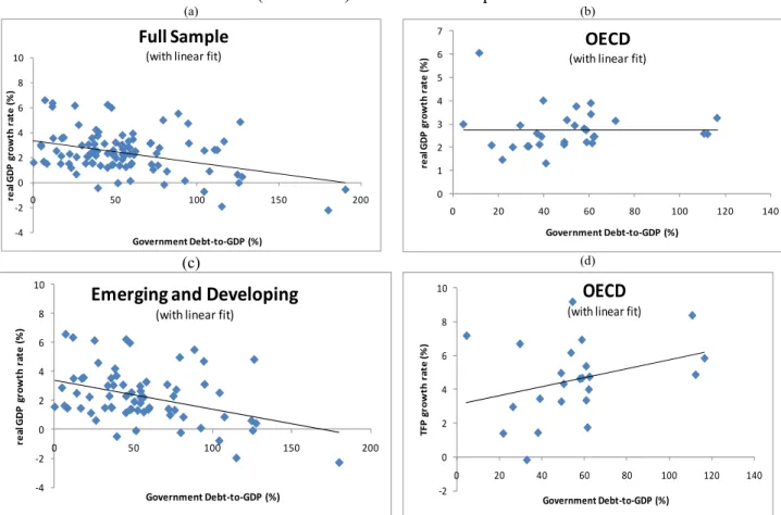
Since we are largely interested in the relationship between growth (and TFP) and debt,

it is instructive to aggregate our data into one big cross-section spanning from 1970-2008

and analyse some scatter plots. Figure 1.a shows per capita real GDP growth against the

ratio of government debt-to-GDP for the full sample. It seems that a negative relationship

between the two variables can be extracted, attested by a linear fit. Figure 1.b looks at the

OECD only but in this case, no clear relationship is found. Lastly, when taking the

sub-sample consisting of emerging and developing countries – Figure 1.c - we also find some

evidence of a negative relationship. If one takes a quadratic fit instead (not shown), to

account for a possible non-linear behaviour between debt and growth, the 95% confidence

interval includes slightly more countries.

[Figure 1] _____________________________

10

We find roughly a similar picture (not shown) when plotting the growth rate of TFP

against the ratio of government debt-to-GDP for the full sample and emerging and

developing sub-sample, that is, a negative relation. However, our graphical representation

suggests a positive relationship between TFP growth and the debt-to-GDP ratio for the

OECD sub-sample (Figure 1.d). In addition, from the Kernel density estimates (Figure 2)

we see that government debt has increased throughout time, which implies an increase of

the size of the government notably when trying to provide the additional services related to

the welfare state.

[Figure 2]

4.2. Results: government debt

4.2.1. Debt-growth relationship

We begin our analysis by estimating a growth regression using annual data, for the

period 1970-2008, using as regressors the initial level of GDP, population growth, trade

openness, private investment (gross fixed capital formation), education and government

debt (our variable of interest). Results (not shown for reasons of parsimony) are in line

with the growth literature, as we find significantly negative coefficients for the initial level

of per capita GDP (conditional convergence hypothesis, confirming the catching-up

process underlying a longer distance to the steady-state) and population growth, and

significantly positive coefficients for trade openness,11 private investment and education

levels. We will refrain from commenting on these results again for the remainder of the

paper as they are generally consistent and robust throughout. As for the debt-to-GDP ratio

evidence points to a statistically significant negative relationship with GDP per capita

growth rates for the full sample (pooled OLS and outlier robust estimators).12

In is important to acknowledge that private credit may bear a complementary

relationship with government debt, notably in the context of economic growth. Therefore,

we have included an interaction term between a measure of credit issued to the private

sector by banks and other financial intermediaries (divided by GDP), excluding credit

given to the government, government agencies and public enterprises, and government

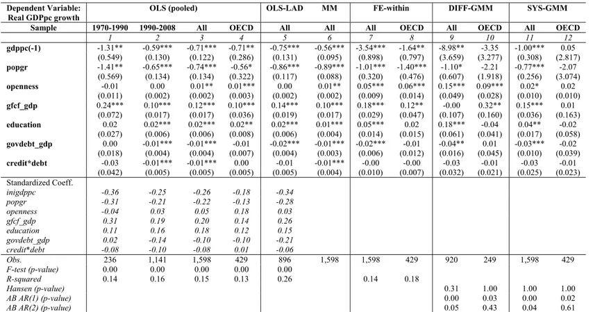
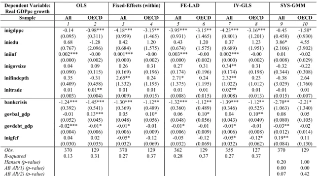
debt-to-GDP ratio. In Table 1 we still get statistically significant negative estimates of the

_____________________________ 11

This translates the successive openness process to international trade flows (removal of trade barriers and other sort of protectionism duties) by many countries, which has been intensified over the last few decades. 12

debt-to-GDP ratio on output growth and, additionally, a negative coefficient for the

interaction term, meaning that the higher the household’s debt burden coupled with higher

government debt, the lower output growth will be. As a robustness exercise we have also

estimated a model excluding the debt-to-GDP ratio, but explicitly including private credit

and the interaction term between the two variables. Results (not shown) suggest that

private credit by itself has a statistically positive effect on growth, however, the interaction

term yields statistically negative coefficients for the all sample which are robust across

econometric specifications (OLS, FE and SYS-GMM). The negative coefficient makes not

only the effect of the debt-to-GDP ratio conditional on the level of private credit, but vice

versa. In fact, it implies that private credit itself boosts growth given a low level of the

debt-to-GDP ratio. However, the negative coefficient on the interaction term has the

interesting implication that there exists a threshold level of the debt ratio above which

private credit can actually dampen growth.

[Table 1]

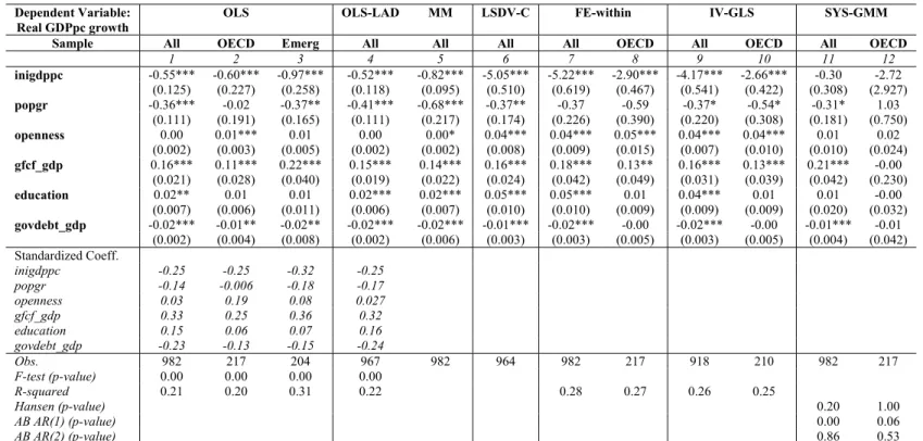
For the remainder of the paper we focus on 5-year averages, as common practice in the

literature. Regarding the full sample we find evidence that an increase in the debt-to-GDP

ratio is detrimental to output growth and this is robust across econometric specifications, as

reported in Table 2.

[Table 2]

Moreover, for the OECD sub-group, the same conclusion seems to apply when running

pooled OLS (and the coefficient is now significant at 5% level). It is instructive to briefly

discuss the size of the standardized coefficients – these indicate the relative importance of

the variables included in the model: a big impact comes from the initial level of per capita

GDP as well as from the population growth rate; private investment also accounts for a

sizeable share; and the negative impact of the debt-to-GDP ratio is confirmed.

In order to explore nonlinearities we re-run the same model with a quadratic-debt-term

included as an additional regressor. Results (not shown) do not provide evidence of any

significant quadratic-debt-term. As a robustness exercise, we have included also credit to

the private sector in our 5-year averages dataset and the same conclusions as for the use of

annual data apply. We have redone these estimations taking potential GDP growth as an

alternative dependent variable.13 In particular, we took the smoothed or detrended GDP

series extracted for each country making use of i) the Hodrick-Prescott, ii) the Baxter-King _____________________________

13

and iii) the Christiano-Fitzgerald random walk filters. Computing the growth rates of these

new series and using them as alternative dependent variables, yields similar results.

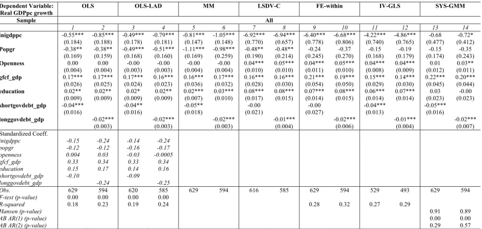
An interesting issue to explore is debt maturity, which we did using information from

the World Bank.14 Table 3.a shows that when short-debt-to-GDP ratio is included in our

growth specifications we still get a negative and statistically significant coefficient (for the

full sample). The same applies when long-term debt is used instead.

[Table 3.a]

In addition, we also assessed the impact of short- and long-term debt, as shares of the

total level of debt.15 In this case we obtain a positive and statistically significant coefficient

(at the 1% level) for the short-debt-to-total debt ratio across different econometric

specifications (being the long-debt-to-total-debt the complement, it naturally yields a

negative coefficient).

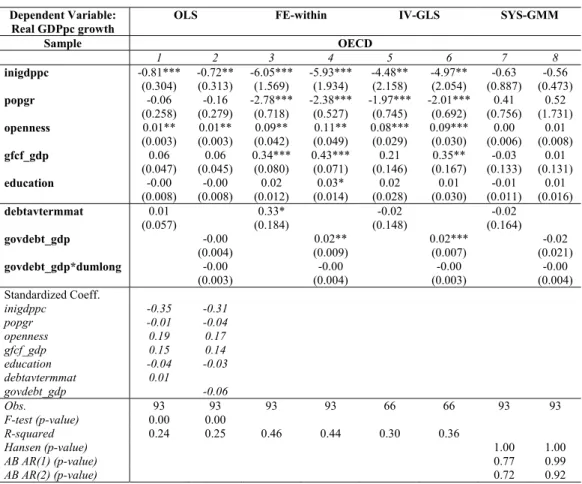
Due to limitations in data retrieved from the WDI, we used the OECD’s own measure

of average debt to maturity (in years) to construct additional dummy (binary type)

variables. For the average maturity above 5 years we have classified it as long-term debt

(dumlong) and attributed a value 1; the complement (short- and medium-term) takes the

value zero. Table 3.b presents the results from these estimations. In only one case we find

evidence supporting the claim that the higher debt maturity the higher the economic

growth rate (specification 3). As for the interaction term it appears not to be significant.

[Table 3.b]

Financial crisis

We now turn to a different, but equally important topic. In line with research by

Afonso, Gruner, Kolerus (2010) on fiscal developments and financial crisis, we take the

Laeven and Valencia’s (2010) database on banking, debt and currency crisis and study the

relevance of these phenomena, when interacted with the debt-to-GDP ratio, in explaining

differences in output growth. According to Easterly (2001), econometric tests and fiscal

solvency accounting carried out in his paper confirm the important role of debt crises.

Table 4 presents the results from adding govdebt_gdp with an interaction term for each type

of crisis introduced one at a time, plus a dummy variable (available in the same dataset)

taking the value 1 when a debt restructuring occurred and zero otherwise. The first aspect to

notice is that govdebt_gdp retains its negative and statistically significant. We do find some

evidence supporting the detrimental effect of financial crisis when associated with higher

_____________________________ 14

Given data availability a number of observations were lost due to data transformations. 15

government debt-to-GDP levels on output growth, in particular those related to debt and

currency crisis (robust across econometric methodologies).

For the OECD sub-group (not shown) we loose statistical significance of the

debt-to-GDP variable entirely, but we retain statistically negative coefficients for most interaction

terms with different types of crisis (in pooled OLS and FE cases; not in the SYS-GMM

though). Moreover, we now have evidence of negative effects of both banking crisis and

debt restructuring operations on per capita GDP growth. This seems to be in line with

Reinhart and Rogoff’s (2009) finding that banking crises are typically accompanied by

large increases in government debts.

[Table 4]

According to Gupta’s et al. (2005) study of 39 low income countries (during the 1990s)

initial conditions also have a bearing on the nexus between fiscal variables and growth, an

avenue is also explored by Kumar and Woo (2010). Therefore, we similarly include the

initial government size (from Gwartney and Lawsson, 2006), in light of the robust results

obtained by Sala-i-Martin et al. (2004).16 In addition, we include initial trade openness,

initial financial depth (llgdp) and initial inflation (all averaged over each time period). A

measure of banking crisis incidence is also considered as we have shown it is important

determinant. The fiscal deficit is included to take into account the finding that fiscal

deficits are negatively associated with longer-run growth (see, Fisher (1993) and Baldacci

et al. (2004)).

From Table 5 it stands out that banking crisis have indeed a negative impact on output

growth which is robust across econometric specifications (as attested before). The budget

balance is positive and statistically significant in four specifications for the OECD sample,

which would imply that a fiscal consolidation promotes growth in a non-Keynesian fashion

in those cases.17 As before, the debt-to-GDP ratio appears with negative and a significant

coefficient for the whole sample and mostly insignificant for the OECD sub-group. As a

robustness exercise we have repeated the analysis without initial conditions of the

regressors previously included (apart from inigdppc) – hence, replaced with variables

averaged over each 5-year period –, and results didn’t change.

[Table 5]

Another exercise worth while conducting is an assessment of the sensitivity degree of

the different explanatory variables included in our regressions. We have re-run the

_____________________________ 16

Fiscal sustainability can also be a motivation, in line with Woo (2003) and Huang and Xie (2008). 17

estimations without the budget balance (due to possible collinearity with either government

debt or government size) and inflation (which proved not to be significant in the regression

with initial conditions; but statistically negative in the first robustness exercise). Such

additional findings confirm the negative effect to debt-to-GDP ratio for the full sample and

for the OECD (the latter when running SYS-GMM).

4.2.2. Debt thresholds

High levels of government debt may affect the allocation of resources, hence growth

and productivity. In this sub-section we study the effect of different debt-to-GDP ratio

thresholds on growth. We followed Table’s 5 setting in terms of initial conditions of the

regressors. In addition to govdebt_gdp included in each specification, we interact this

variable with a dummy variable (dum30) taking the value 1 if the debt-to-GDP ratio was

below 30 at a certain point in time, between 60 and 90 (dum3060) or above 90 (dum90),

respectively. We find that the 30% debt threshold is positive and statistically significant at

1 percent level in one pooled OLS, one FE, and SYS-GMM estimation for both the whole

sample, and for the OECD sub-group. For the full sample having a debt-to-GDP ratio

above 90 affects negatively growth.18

In order to have a visual image, we plot the cross-sectional average of per capita GDP

growth rates for these levels of debt-to-GDP ratios for the entire sample as well as the

OECD and emerging economies sub-groups in Figure 3. Low debt is defined as having

govdebt_gdp below 30% and high debt as a level above 90%. A consistent pattern is

present, namely countries with low debt ratios grow faster (which is also true for the

emerging sub-group). No significant difference is found with respect to OECD economies.

[Figure 3]

We also computed the impact on growth of a given proportional increase in the

debt-to-GDP ratio. This was undertaken to allow an appropriate comparison of the impact of

government debt on growth at different levels of debt and reflects the fact that an increase

in the ratio from 10 to 20 percent constitutes a doubling, while an increase from 100 to 110

percent raises it only by one-tenth. Table 6 summarizes the results for debt ratios in three

groupings: <30%, 30-60% and > 90%. For each of these grouping we obtained the sample

average debt ratio (row 1), and then multiplied a given increase (10%) in this ratio, by the

estimated coefficient of the interaction term (row 2, based on the different estimation

_____________________________

18

techniques). The results (row 3) indicate that the higher the level of the debt ratio, the

higher the negative impact on output growth. For instance, a 10 percent increase in the debt

ratio in countries with debt ratio above 90 percent is associated with a decline in growth of

0.27 percent, while an identical increase in the debt ratio in the 30-60 percent group is

associate with a decline is growth around 0.08 percent.

[Table 6]

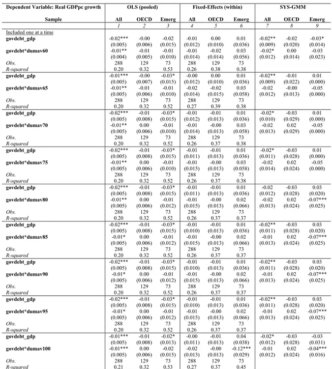
In Table 7 we run additional regressions with the debt ratio interacted with dummy

variables taking the value 1 if the average debt ratio of a particular country over that

country’s time span is above 60 (dumav60), above 65 (dumav65) until we reach the level

of 100 (dumav100). For reasons of parsimony we only report the coefficients of interest

and not the full set of estimates. The results show that for the whole sample, irrespective of

the threshold level included in the regression, we always find the debt-to-GDP ratio having

a negative and statistically significant effect on growth for the pooled OLS and SYS-GMM

specifications. Similarly, for emerging countries we have the same result. Nothing can be

said with respect to the OECD sub-group.19 The interaction terms in specification 1 (for the

full sample) suggest that having average debt ratios above 60 further increases the adverse

impact of debt on output growth. Indeed, we find interaction terms with statistically

significant negative coefficients in 8 out of 9 regressions for the full sample.

[Table 7]

Endogenous debt threshold

In the context of defining a plausible debt threshold level, other than specifying it in a

purely ad-hoc way, we now explore the endogenous determination of the debt-to-GDP

threshold ratio which is the threshold value in the empirical model that provides the best fit

by maximizing its likelihood. Based on a reduced form growth equation allowing for the

presence of multiple equilibrium (like in Strubhaar et al., 2002), we can employ Hansen’s

(1996, 2000) techniques to a (generalized) threshold regression of the form:

01 11 0 21 1

02 12 0 22

i it

it it

i it

y X if G

y y

y X if G

γ γ γ γ

γ γ γ γ

−

+ + → > − =

+ + → < (2)

whereγij,i,j=0,1,2 are regression coefficients and γ is a threshold value that splits the

sample in two halves. X_it is a vector of control variables consisting of population growth,

_____________________________ 19

openness, education and investment. The main innovation of the empirical part is to

estimate γ endogenously and then split the entire sample accordingly (by examining

whether a country performed better (over-performer) or worse (under-performer) than its

country-specific growth projection). The threshold variable, G, will be the government

debt ratio.

Equation (2) has an econometric correspondence: a threshold regression model. This

model estimation procedure involves three steps: i) estimating the sample split threshold

value; ii) testing whether the endogenously determined sample split value is significant;

and iii) performing conventional hypothesis tests.

The endogenously determined sample split is estimated by minimizing mean square

errors,

) ( )' ( min

arg _{i i}

Q q

q e q e

i∈ =

γ (3)

where q_i is the value of the threshold variable (government debt) of region i, Q is the set

of all different values of q_i in the sample, γ is the estimated threshold value of q_i, and

) (q_i

e is the vector of OLS residuals of the regression (2) if the sample is split in

observations larger or smaller than q_i, and each sample half is estimated separately.

The significance of the sample split could be obtained from a conventional structural

break test (Chow test). However, Davies (1977) argued that this test is invalid in the

present context, because it assumes that the sample split γ is known with certainty, while

we estimate it endogenously. A Chow test would not take into account the estimation error

of γ and the uncertainty whether the threshold exists under the null hypothesis. Hansen

(1996) suggests a Supremum F-, LM- or Wald-test, which has a non-standard distribution

dependent on the sample of observations. The critical values can be obtained by a

bootstrap.

Estimating (2) with cross-sectional 5-year averages and with the annual samples

(correcting for heteroskedasticity)20 yields an estimated threshold value γ =59.305 and a

corresponding Supremum Wald-test of 27.89 whose p-value is 0.079, indicating a

significant sample break for the full sample.21

_____________________________ 20

We thank Dieter Urban for kindly making his original code available, which was adaptated to our particular needs.

21

If we take the roughly 60% debt threshold just computed and attempt to summarize

GDP growth based on this information we have in Figure 4 a visual representation that

allows us to draw some meaningful conclusions. In particular, either picking the 60% debt

threshold or the 3% budget deficit level, splitting the sample results in having countries

with higher debt ratios, and higher budget deficits, associated with lower growth rates. On

the other hand, countries with lower debt ratios and lower fiscal imbalances have higher

growth rates.

[Figure 4]

Financial development

One additional issue to keep in mind when investigating the relationship between

government debt and growth is the level of financial development. The negative impact of

government debt on growth could conceivably be stronger in countries with more

developed financial systems, translating, for example, a higher private debt stock and

associated burdens (as already partly explored before with the inclusion of private credit).

Therefore, we proxy financial development with different measures computed using

PCA (see Appendix 1.b for the computation of these variables). As a first exercise, we run

a regression including the previous set of initial regressors plus our overall measure of

financial development (fd) and the latter interacted with the previously constructed

dummies for the debt ratio threshold. In a second exercise, similarly to Table 7, we run

independent regressions one at a time with a proxy for financial development and its

interaction with the above 60% debt threshold, which we have computed as the

approximate threshold level.22

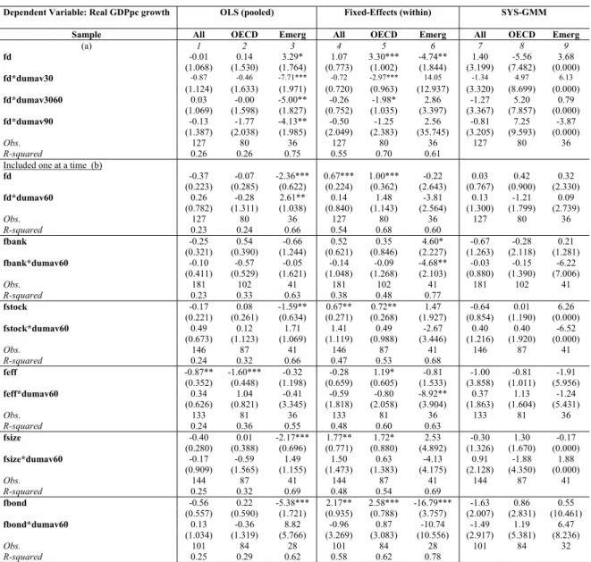
The evidence in Table 8 (panel a) suggests that those proxies and the interaction terms

are statistically stronger in emerging countries. Results from the first exercise suggest that

overall financial development has a positive effect on growth, but not when interacted with

debt ratios, and the same is true for the OECD sub-group (according to the fixed-effects

estimation). From the second exercise (Table 8, panel b), financial development, stock

market development, financial size, financial efficiency, and bond market development

essentially affect positively growth in the OECD sub-group. For emerging countries if the

debt-to-GDP ratio is above 60% both the banking sector development and financial

efficiency have a detrimental impact on output growth.

find a debt threshold of 58.14% highly significant (at 1% level). Finally, for the emerging countries sub-group a threshold of 79.11% was found for the debt-to-GDP ratio (significant at 1% level).

22

[Table 8]

4.3. Debt-TFP relationship: a growth accounting approach

A detailed growth accounting exercise was also undertaken – based on the measures of

TFP and capital stock per worker (see Appendix 1.a) – through which government debt

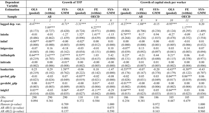
influences growth. Table 9 presents panel regression estimates on the growth rate of TFP

and capital stock per worker. Similarly to per capita GDP growth we find that the level of

financial development affects positively both TFP and capital stock growth rates. While

banking crises have a positive effect on TFP growth, they have a detrimental effect to the

capital stock growth rate. Moreover, the budget balance appears with a negative coefficient

for the OECD sample when explaining TFP growth but positive ones when explaining

capital stock growth rates. Furthermore, the debt-to-GDP ratio has positive effects when

considering both samples for TFP growth rates.

[Table 9]

Regarding the impact of debt ratios on private and public investment (not shown), our

results suggest that banking crises and debt ratios have statistically significant negative

effects in both cases. However, the impact of the budget balance is distinct: for private

investment a higher debt ratio has a positive effect, whereas a higher debt ratio is

associated with lower levels of government fixed capital formation.

4.4. Cross-sectional dependence

As discussed before, it is natural to suspect of the existence of cross-sectional

dependence across homogeneous groups of economies. Therefore, we use Pesaran’s CD

test (standard growth equation, with a basic set of controls, the debt ratio, and fixed effects)

for the OECD and Euro-area sub-samples. We find statistics of 15.26 and 10.26;

respectively corresponding to p-values of zero in both cases, rejecting the null hypothesis

of cross-sectional independence.

In Table 10 we run benchmark type growth regressions for the two sub-samples using

either a Driscoll Kraay robust estimation approach or Pesaran’s Common Correlated

Effects Pooled Estimator (CCEP). We examine three main variables of interest: debt ratio,

the change of the debt ratio, and average debt maturity (using the OECD measure).

Similarly to our earlier results, we find that government debt has a negative effect on

growth for the OECD sub-group using Driscoll-Kraay robust estimation, but not under the

associated with higher debt ratios. When running the CCEP estimator the debt maturity

yields statistically significant positive coefficients, reinforcing our results in Table 3.b,

which appeared to be weak.

[Table 10]

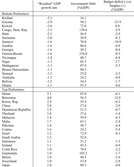
4.5. “Above” and “below” average performers vis-à-vis fiscal thresholds

To gain additional insight on the relationship between fiscal developments and

economic performance, we briefly review some country-specific details related to the

regression results reported above (in particular the regression equation corresponding to

specification 1 in Table 2). The main purpose of this exercise is to see if any definite trend

can be observed with respect to government debt and budget deficits and the level of

economic performance of the so-called “above-average performers” and “below-average

performers” (countries), vis-à-vis the fiscal thresholds.

For the full sample we identified above-average and below-average performing

countries on the basis of the difference between their actual and predicted values of per

capita GDP growth rates. In line with Nelson and Singh (1994) countries whose actual

growth rates exceeded their predicted growth rates by 1% or more were classified as

“above-average” performers, and countries that fell short of the predicted growth by a

similar percentage (or more) were categorized as “below-average” performers. The list of

countries in both categories is reported in Table 11. In both cases we run the regression

using government debt-to-GDP ratios as the included fiscal variable of interest. The table

shows the residual of the per capita GDP growth rate, the government debt ratio, and the

budget balance ratio for these groupings of countries.

[Table 11]

From examination of the results in Table 11 there is no clear-cut or direct connection

between these aggregates. In particular, we cannot conclude that the “above-average”

performers (higher residuals in this case) have had necessarily lower debt ratios or budget

deficits and that the “below-average” performers generally experienced larger debts and

deficits. For example, we have “below-average” cases (negative residuals) with low levels

of government debt and even budget balance surpluses. Conversely in the “above-average”

category we find countries such as Israel with both a high debt ratio and a substantial

budget deficit. If one isolates the group of OECD countries (not shown) we also have a

mixed picture with, for instance, Greece being in the “above-average” category but with a

the “below-average” category although it has relatively small debt ratio (35.1%) and a

budget deficit of 1.1% GDP. Still for OECD countries, the higher the computed residuals

in absolute terms, the lower the debt-to-GDP ratio. The same is true for the budget balance

in the “above–average” Performers: the higher the computed residuals, the higher the

budget balance (or the lower is the deficit).

Finally, and in order to summarise the overall effect of government debt on economic

growth it is possible to build a density chart of all the statistically significant estimated

coefficients, as depicted in Figure 5, where the left skewed plot confirms the global

negative effect of government debt on economic growth.

[Figure 5]

5. Conclusion

We have used cross-sectional/time series data for a panel of 155 developed and

developing countries for the period 1970-2008, in order to assess the potential linkage

between fiscal policy developments and economic growth. More specifically, we used

growth equations and growth accounting techniques and focussed also on a number of

econometric issues that can have an important bearing on the results, notably, simultaneity,

endogeneity, the relevance of nonlinearities, and threshold effects.

Our empirical results confirm the negative effect of the government debt ratio for the

full sample in our dataset. This result is robust across econometric methodologies and the

inclusion of different sets of regressors. We don’t find evidence supporting a Laffer-type

relationship, as a quadratic debt term was found to be statistically insignificant. Moreover,

when taking debt maturity into account it differs whether one has short or long-term debt

as percentage of GDP or as percentage of the total debt level. In the first case, we get

statistically negative coefficients for both the short- and long-term debt across different

econometric specifications for the full sample. Using the second definition, we find that

short-term debt positively affects growth. For the OECD sub-group only, we have the

result that the longer the average maturity of government debt the higher growth will be.

Using the IMF’s database on financial crisis we confirm their detrimental effect of

growth, but that is further worsened if interacted with high debt-to-GDP ratios. When the

budget balance is included in the equation to be estimated we consistently get positive

coefficients, which implies that, in those cases, a fiscal consolidation promotes growth in a

non-Keynesian fashion. In addition, the higher the household’s debt burden coupled with

With respect to the analysis of different government debt thresholds, countries with

debt ratios above 90% of GDP are associated with lower economic growth rates when

compared with countries that maintained an average debt ratio below 30% of GDP over the

period under scrutiny. In particular, for the latter group, the growth impact of a 10%

increase in the debt ratio is 0.1% whereas for the former group of countries that effect

amounts to -0.2%. Using Hansen’s endogenous determination of the threshold debt ratio

we find that, for the full sample we get a value of 59% of GDP, more specifically 58% of

GDP for the Euro area, and for emerging countries a slightly bigger value of 79% of GDP.

Regarding the level of financial development when interacted with government

debt-to-GDP, our results show that it positively affects growth in the OECD sub-group, and the

same is valid for stock market development, financial efficiency and bond market

development (after controlling for the debt-to-GDP ratio set at 60%).

On a growth accounting perspective, higher debt ratios are beneficial to TFP growth,

and for the growth of capital stock per worker, whereas they are detrimental to the levels of

private and public investment. The budget balance appears with positive contributions for

the TFP growth, capital stock growth and private investment. Finally, most results are

confirmed even after we account for cross-section dependence.

References

Abbas, A., Belhocine, N., ElGanainy, A., Horton, M. (2010), “A Historical Public Debt

Database”, IMF Working Paper No. 10/245.

Afonso, A. (2010). “Expansionary fiscal consolidations in Europe: new evidence”, Applied

Economics Letters, 17 (2), 105-109.

Afonso, A., Furceri, D. (2008). “EMU Enlargement, Stabilisation Costs and Insurance

Mechanisms”, Journal of International Money and Finance, 27 (2), 169-187.

Afonso, A., Gruner, H., Kolerus, C. (2010), “Fiscal policy and growth – do financial crises

make a difference”, ECB WP 1217.

Bai, J. (2009), “Panel data models with interactive fixed effects”, Econometrica, 77(4),

1229-1279.

Baldacci, E., Clements, B., and Gupta, S. (2003), “Using fiscal Policy to Spur Growth.”

Finance and Development, December, pp.28-31.

Barro, R. and Lee, J.W. (2010), “International data on educational attainment, updates and

Bowsher, C. G. (2002) "On testing overidentifying restrictions in dynamic panel data

models", Economics Letters, 77(2), 211-220

Bruno, G. (2005), “Approximating the bias of the LSDV estimator for dynamic unbalanced

panel data models”, Economics Letters, 87(3), 361-366.

Checherita, C. and P. Rother (2010), “The impact of high and growing government debt on

economic growth - an empirical investigation for the euro area”, ECB Working Paper

No. 1237.

Coakley, Jerry, Fuertes, Ana-Maria & Smith, Ron, 2006. "Unobserved heterogeneity in

panel time series models", Computational Statistics & Data Analysis, 50(9), 2361-2380

Corsetti, G., Kuester, K., Meier, A., Müller, G. 2010. "Debt Consolidation and Fiscal

Stabilization of Deep Recessions," American Economic Review, 100 (2), 41-45.

Dar, A. Amirkhalkhali, S. (2002), “Government size, factor accumulation and economic

growth: evidence from OECD countries”, Journal of Policy Modeling, 24, 679-692.

Davies, R.B., (1977), Hypothesis testing when a nuisance parameter is only present under

the alternative, Biometrika, Vol. 64, p. 247-54.

de la Fuente, A. (1997), “Fiscal Policy and growth in the OECD”, CEPR WP, No 1755

Demirgüç-Kunt, A. and R. Levine (1996), “Stock markets, corporate finance and economic

growth: An overview”, World Bank Economic Review 10(2), 223-240.

Demirgüç-Kunt, A. and R. Levine (1999), “Bank-based and market based financial

systems: Cross-country comparisons”, World Bank Policy Research working paper no.

2143.

Driscoll, John and Aart C. Kraay, 1998. "Consistent Covariance Matrix Estimation With

Spatially Dependent Panel Data", The Review of Economics and Statistics, 80(4),

549-560

Easterly, W. R. (2001), “The Lost Decades: Developing Countries Stagnation in Spite of

Policy Reform 1980-1998”, Journal of Economic Growth, 6(2): 135-157.

Eberhardt, M., Helmers, C. And Strauss, H. (2010), “Do spillovers matter when estimating

private returns to R&D?” Economic and Financial Reports 2010/1, EIB.

Eberhardt, M. and Teal, F. (2011), “Econometrics for Grumblers: A new look at the

literature on cross-country growth empirics”, Journal of Economic Surveys, 25(1),

109-155.

Fisher, S. (1993), “The role of macroeconomic factors in growth”, Journal of Monetary

Gemmell, N. (2004), “Fiscal Policy in a Growth Framework”, In: T. Addison and A. Roe,

eds. Fiscal Policy for Development: Poverty, Reconstruction and Growth. Great Britain:

Palgrave Macmillan, 149-176

Gollin, D. (2002), “Getting Income Shares Right,” Journal of Political Economy, 110 (2),

458-74.

Gwartney, J. and Lawson, R. (2006), “Economic Freedom of the World: 2006 Annual

Report”, Vancouver: The Fraser Institute.

Hall, R.E. and Jones, C. (1999), "Why do some countries produce so much more output per

worker than others?", Quarterly Journal of Economics, 114, 83.116.

Hansen, Bruce E., (1996), Inference when a nuisance parameter is not identified under the

null hypothesis, Econometrica, Vol. 64, p. 413 - 430.

Hansen, Bruce E., (2000), Sample splitting and threshold estimation, Econometrica, Vol.

68, p. 575-603.

Heston, A., Summers, R. and Aten, B., Penn World Table Version 6.3, Center for

International Comparisons of Production, Income and Prices.

Huang, H., Xie, D. (2008), “Fiscal sustainability and fiscal soundness”, Annals of

Economics and Finance, 9(2), 239-51.

Huang, H. (2010), Determinants of Financial Development, Palgrave MacMillan.

Kapetanios, G., Pesaran, M. H., Takashi, Y. (2009), “Panels with non-stationary

multifactor error structures”, unpublished working paper, updated version of IZA WP

No. 2243.

Kiviet, J. (1995), “On bias, inconsistency and efficiency of various estimators in dynamic

panel data”, Journal of Econometrics, 68(1), 53-78.

Klenow, P. and Rodriguez-Clare, A. (2005), "Externalities and Growth", Handbook of

Economic Growth, Philippe Aghion & Steven Durlauf (ed.), chapter 11, 817-861.

Kormendi, R.C and P.G Meguire (1985), “Macroeconomic determinants of growth: Cross

country evidence”, Journal of Monetary Economics 16, 141-164.

Kumar, M. and Woo, J. (2010), “Public debt and growth”, IMF WP 10/174.

Landau, D. (1983), “Government Expenditure and Economic Growth: A Cross Country

Study”, Southern Economic Journal 49, 783-792.

Modigliani, F. (1961), “Long-run implications of alternative fiscal policies and the burden

Nelson, M.A. and R.D. Singh (1994), “Deficit-Growth Connection: Some Recent Evidence

from Developing Countries”, Economic Development and Cultural Change 43(1):

167-91.

Pesaran, M. H. (2006), “Estimation and inference in large heterogeneous panels with a

multifactor error structure”, Econometrica, 74(4), 967-1012.

Pesaran, M. H. (2007), “A simple panel unit root test in the presence of cross section

dependence”, Journal of Applied Econometrics, 22(2), 265-312.

Pesaran, M. H. (2009), “Weak and strong cross section dependence and estimation of large

panels”, Keynote speech, 5th Nordic Econometric Meeting, Lund, 29th October.

Pesaran, M. H., Tosetti, E. (2007), “Large panels with common factors and spatial

correlations”, CESIFO WP No. 2103

Pesaran, M.H. (2004), “General diagnostic tests for cross section dependence in panels”,

Cambridge Working Papers in Economics, 0435, University of Cambridge.

Psacharopoulos, George (2004), "Economies of education: from theory to practice,"

Brussels Economic Review, ULB -- Universite Libre de Bruxelles, 47(3-4), 341-358.

Psacharopoulos, George and Harry Patrinos (2002), "Returns to Investment in Education:

A Further Update.", Education Economics, 12(2), 111-134

Ram, R. (1986), “Government Size and Economic Growth: A New Framework and Some

Evidence from Cross-Section and Time Series Data”, American Economic Review, 76,

191-203.

Reinhart, C., Rogoff, K. (2009), “The aftermath of financial crises”, American Economic

Review, 99(2), 466-72.

Rodrik, D. (1998), "Why Do More Open Economies Have Bigger Governments?", Journal

of Political Economy, 106(5), 997-1032

Roodman, D. (2009), "A Note on the Theme of Too Many Instruments", Oxford Bulletin

of Economics and Statistics, 71(1), 135-158

Rousseeuw , P. J., A. M. Leroy, “Robust regression and outlier detection”, John Wiley &

Sons, Inc., New York, NY, 1987.

Rousseeuw, P. J. and Van Driessen, K. (1999), “A Fast Algorithm for the Minimum

Covariance Determinant Estimator”, Technometrics, 41, 212-223.

Saint-Paul, Gilles (1992), "Fiscal Policy in an Endogenous Growth Model", The Quarterly

Journal of Economics, 107(4), 1243-59

Sarafidis, V., Wansbeek, T. (2010), “Cross-sectional dependence in panel data analysis”,

Schclarek, Alfredo A. (2004), “Debt and Economic Growth in Developing and Industrial

Countries”, Working Papers 2005:34, Lund University

Straubhaar, T,, Suhrcke, M., Urban, D. (2002), "Divergence – Is it Geography?"

Development Working Papers 158, Centro Studi Luca d\'Agliano, University of Milano

Woo, J. (2003), “Economic, political and institutional determinants of public deficits”,

Journal of Public Economics, 87(3), 387-426.

Yohai, V. J. (1987), “High Breakdown-Point and High Efficiency Robust Estimates for

Regression”, Annals of Statistics 15, 642-656.

Appendix 1.a Growth Accounting - TFP

For human capital (H), we follow Hall and Jones (1999) and Klenow and

Rodriguez-Clare (2005) in giving a larger weight to more educated workers:

H =exp(φ(E)) (A1)

where E is the average years of schooling; and the function φ(E) is piece linear with slope

of 0.134 for E≤4, 0.101 for 4<E≤8 and 0.068 for 8<E. The wage of a worker with E

years of education is proportional to her human capital. Since the wage-schooling

relationship is widely believed to be log-linear, this would imply that H and E would have

a log-linear relation as well, such asH =exp( * )φ E . International data on education-wage

profiles (Psacharopoulos, 1994) suggests that in Sub-Saharan Africa the return to one extra

year of education is about 13.4%, the world average is 10.1% and the OECD average is

6.8%. We estimate the capital stock, Ky, using the perpetual inventory method:

Kyt =It +(1−δ)Kyt−₁ (A2)

where I_t is the investment and δ is the depreciation rate. Data on I_t are from PWT 6.3 as

real aggregate investment in PPP. We estimate the initial value of the capital stock (Ky₀),

in year 1950 as I₁₉₅₀/(g+δ) where g is the average compound growth rate between 1950

and 1960, and δ is the depreciation rate (set to 7% for all countries and years).

We construct two different measures of TFP: one for a smaller sample of countries,

which have investment data from 1950 onwards and TFP figures go from 1960 till 2007,

and another, larger sample, for countries which have investment data from 1960 onwards

and TFP figures go from 1970 till 2007. TFP was then based on a Cobb-Douglas aggregate

production function of the typeY = AKα(HL)1−α, following the neoclassical tradition,