Decentralized solar PV generation forecast based on peer-to-peer approach

FACULDADE DE CIÊNCIAS

DEPARTAMENTO DE ENGENHARIA GEOGRÁFICA, GEOFÍSICA E ENERGIA

Decentralized Solar PV generation forecast based on

peer-to-peer approach

Luís Carlos Claudino Teixeira da Silva

Mestrado Integrado em Engenharia da Energia e Ambiente

Dissertação orientada por:

Miguel Centeno Brito (FCUL)

Acknowledgment

I wish to acknowledge those who, either by chance or simple misfortune, were involved in my dissertation.

I want to begin by thanking my mentors, Rodrigo Amaro and Professor Miguel Brito for the trust, the support given throughout the project and for helping me to overcome all the doubts that have appeared.

I would also like to thank Eng. Margarida Pedro and Eng. Filipa Reis and the entire team from the EDP Inovação, for the opportunity of this project and for accepting me.

To my family, for being my support. Especially my mother, with her big words, never let me down.

Finally, my great friend, João Costa, for giving me the strength and support along this work. And to all my colleagues and friends who were present for me, like Francisco Pinto and Nuno Pego.

Resumo

Atualmente, cerca de 80% de energia consumida provêm de fontes não renováveis. O aumento da concentração de gases de efeito de estufa e poluentes na atmosfera está fortemente relacionado com a conversão de combustíveis fósseis em eletricidade, calor e a sua utilização em veículos. Este percurso leva a mudanças climáticas que vão perturbar o delicado equilíbrio dos ecossistemas e pode facilmente levar várias espécies de animais e plantas à sua extinção.

A utilização de fontes de energia renováveis como solar ou o vento para a produção de energia elétrica pode fornecer uma solução fazível para a redução de emissão de gases de efeito de estufa, já que são livres de emissões poluentes para a atmosfera, e desta forma salvaguardar futuras gerações. A energia solar, em particular produção fotovoltaica (PV), pode satisfazer as necessidades elétricas de toda a humanidade. Na última década, sistemas PV têm vindo a aumentar o seu potencial, com a integração de células PV em edifícios de habitação e serviços. Em 2015, o mercado PV ultrapassou vários recordes com a sua expansão global, tendo nesta altura uma capacidade total instalada de cerca de 227 GW, dez vezes maior do que em 2009. Em 2016 voltaram-se a bater recordes com um aumento de cerca de 75 GW.

Em Portugal a tecnologia PV tem sido, de todas as tecnologias renováveis, a que mais cresceu, sendo praticamente inexistente em 2006 para uma capacidade instalada de 467 MW no fim de 2016. Cerca de 72 MW estão instalados no sector residencial. Na Europa cerca de 20 GW está instalado no sector residencial, para um total da ordem de 50 GW (no mundo).

A introdução desta nova tecnologia na rede elétrica levanta desafios devido ao seu carácter não controlável, causando vários problemas para os operadores da rede elétrica, como por exemplo problemas de fluxo de potência inversa ou de controlo de voltagem.

As previsões de radiação solar e/ou produção fotovoltaica proporcionam um modo para os operadores de rede controlarem e gerirem os balanços de produção e de consumo de energia de forma a otimizar o processo e não terem de usar as suas reservas de segurança, reduzindo custos.

Com o aumento de produção PV distribuído, a necessidade de prever a sua potência produzida é cada vez maior para o operador do sistema distribuição (DSO). Um dos principais objetivos desta dissertação é estudar e desenvolver um modelo de previsão para a produção PV distribuída na perspetiva do DSO. Isto significa que o modelo de previsão criado deve poder ser aplicado a qualquer sistema sem saber os seus detalhes técnicos; os sistemas analisados vão ser considerados como caixas negras, onde apenas a potência instalada, a distância entre sistemas e o seu histórico de produção é conhecido.

Existe uma grande variedade de técnicas de previsão. Como tal foi feita uma filtragem destas técnicas com o objetivo de ter um modelo simples como base de comparação, um modelo eficiente e um modelo mais complexo, mas com um grande potencial. Após uma análise de bibliografia os modelos escolhidos foram a Persistência (usada como um bom modelo de referência), regressões multivariáveis (simples, com resultados bastante satisfatórios) e o modelo de vetores de suporte (que têm tido um acréscimo de desenvolvimento e resultados bastante interessantes).

A Persistência é o modelo que assume que o que está a acontecer no presente se repetirá no futuro. Embora simples, este modelo pode obter melhores resultados do que modelos numéricos de previsão de tempo (NWP) já que para horizontes curtos consegue traduzir uma melhor

(algumas horas ou dias) este modelo começará a obter erros bastantes grandes, mas serve uma base de comparação apropriada para outros modelos.

O modelo de regressões multivariáveis (ARX) é um modelo de regressão linear que incorpora mais do que uma variável independente. Na maioria dos casos as relações principais costumam ser lineares ou, caso não sejam, podem ser assumidas de uma forma satisfatória, e desta forma aplicar este modelo e obter resultados interessantes. As grandes vantagens deste modelo é a sua fácil utilização e implementação, mas pode levantar dificuldades quando temos poucos dados ao fazer um ajuste demasiado fino aos dados de treino e perder a sua capacidade de generalizar para variáveis ainda não conhecidas.

Um modelo mais complexo que também usa regressões é o modelo de vetores de suporte. Este modelo foi inicialmente um modelo orientado para problemas de classificação linear, para separar duas classes através de uma linha reta num plano em outra dimensão, chamado de Hyperplane. Este modelo foi mais tarde usado para problemas não lineares onde foi adaptado para problemas de previsões através de regressões lineares por Vapnik, 1995, passando a chamar-se regressão de vetores de suporte (SVR).

O conceito geral deste modelo é transformar os dados fornecidos para uma outra dimensão onde seja possível fazer uma regressão linear, e depois devolver esta função. Esta transformação para outra dimensão é bastante facilitada graças a facilidade de incorporar o uso de funções kernel já existentes. O único problema é a escolha dos vários kernel que se torna um problema não trivial. Para este trabalho escolheu-se o kernel RBF, o mais usado por outros estudos semelhantes. Os parâmetros principais deste modelo são o épsilon e o cost. Estes parâmetros vão ser coeficientes que vão criar um intervalo onde o que esteja dentro deste será ignorado pelo modelo, olhando este apenas para os que restaram; estes dados que não são ignorados são chamados de vetores de suporte.

Outra forma deste modelo é o nu SVR, que em vez de nos deixar escolher o épsilon, permite-nos escolher a percentagem de vetores de suporte a usar e desta forma ele automaticamente calcula o épsilon a usar. A vantagem desta abordagem é na poupança de tempo computacional a escolher o melhor épsilon, mas com a contrapartida de perder algum controlo sobre o erro do modelo, já que não é possível escolher o épsilon. A grande vantagem do modelo SVR é que de certa forma é imune ao excesso de ajuste dos dados para o treinar já que os parâmetros épsilon e cost evitam isto e consegue obter desempenhos satisfatórios com o uso de poucos dados.

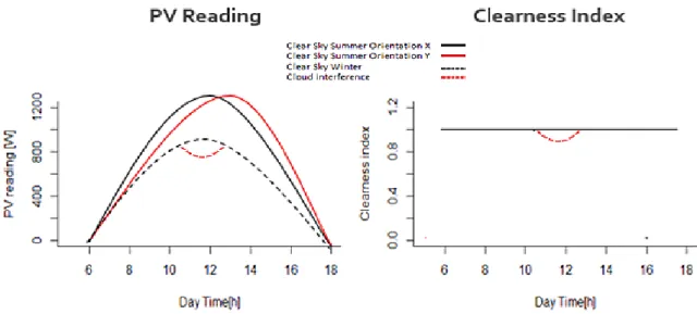
Para a previsão de radiação solar ou produção fotovoltaica é importante considerar o índice de céu limpo. O índice de céu limpo (K) relaciona a condição de um instante totalmente limpo (sem nebulosidade) com a condição real existente. Este índice varia entre K=1, que é um instante sem nebulosidade, e K=0, que representa um instante sem qualquer luz (noite, ou eclipse). O K pode ser usado para isolar a interferência causada pelas nuvens e eliminar os impactos da posição dos módulos ou da variabilidade sazonal. A remoção destes impactos permite a utilização da informação de vários sistemas diferentes de uma forma equivalente. Neste trabalho o K é calculado através da abordagem de Lonij, pela sua simplicidade e a necessidade de apenas do histórico de produção do(s) sistema(s) selecionado(s).

Nesta dissertação os dados usados para desenvolver e testar os modelos de previsão referem-se a Inglaterra, região de East Midlands, para um ano completo (01/07/2015 até o dia 30/06/2016), com um passo de 30 min. Foi realizada uma análise preliminar a estes dados, eliminando as estações com demasiados valores em falta; no final são usados dados de 57 sistemas. Além da previsão da geração individual de cada sistema, foi também considerado testar a previsão para a

Um dos primeiros problemas identificados foi o tempo necessário para a aplicação do modelo SVR. Os dados foram transformados para um passo de 1h de forma a reduzir em metade o número de dados usados. Os parâmetros para o SVR foram reduzidos a cinco hipóteses por parâmetro (épsilon, cost e gamma). Os números de estações previstas do modelo foram reduzidos de 57 a 12 (as 57 estações foram usadas como variáveis pelos modelos para a previsão) e o nu SVR foi utilizado para verificar se a redução no tempo era significativa e se haveria perda de desempenho. Os horizontes estudados foram de 1h até 6h.

O modelo da Persistência foi o primeiro a ser testado. Cada modelo terá inicialmente apenas informações do tempo presente (n = 1), sendo o primeiro caso de estudo, depois adicionando 2 pontos passados (n = 3) e, finalmente, adicionando 4 pontos passados (n = 5).

Em todos os casos de estudo, tanto o ARX quanto o SVR superaram o modelo de Persistência, exceto no quarto caso (n=5), o ARX neste caso, especialmente para horizontes maiores, têm o pior resultado. Os resultados em geral demonstraram que o uso de informações das estações próximas ajuda a precisão da previsão.

Concentrando no caso em que se usa apenas dados do presente (n = 1), a previsão do ARX e SVR, mostra um desempenho muito semelhante, com ligeira vantagem para SVR em horizontes maiores. Um aspeto sistemático na previsão para o caso regional é ter um desempenho menor do que o caso individual para horizontes inferiores, mas quase igual para horizontes maiores. Como a referência de comparação de ambos os modelos (ARX e SVR) é a Persistência e esta melhora no caso regional, devido a soma dos vários sistemas suavizar o comportamento da produção PV, os modelos aparentam ter pior performances para horizontes baixos, o que não se verifica no erro médio quadrático normalizado (nRMSE).

Quando n = 3 e n = 5, o SVR supera o ARX, sobretudo para horizontes maiores, mas com pior desempenho do que o caso de usar apenas informação presente (n = 1). Isso significa que adicionar informação passada apenas teve impacto negativo nos modelos. Isto pode ser uma adversidade de usar dados com um passo de 1 hora e não o passo original de 30 minutos, já que desta forma, para horizonte grandes (4h para cima) o modelo ARX pode perder a sua capacidade de generalizar tendo um ajuste demasiado grande ao treino, devido a redução de alvos na previsão. As nuvens podem ser eventos muito rápidos, portanto, para um melhor resultado, dever-se-ia usar dados de resolução mais alta, já que o passo de 1 hora é uma resolução muito baixa. A principal ideia que pode ser retirada destes casos é que o modelo SVR é um modelo mais robusto do que o ARX e pode lidar melhor com o uso de mais variáveis, não sofrendo de excesso de ajustamento, que parece acontecer no modelo ARX.

O modelo SVR exige uma computação muito mais exigente do que o ARX, sendo o principal problema o processo de otimização dos parâmetros. A alternativa utilizada nu SVR, reduziu consideravelmente esse processo sem perda de desempenho, uma alternativa ótima para o caso em questão, mas se realmente for necessário controlar a quantidade de erro no modelo e ir para o melhor desempenho possível, o épsilon SVR é o modelo escolhido. Estes modelos deveriam ser testados com dados de resolução mais elevada, já que deve melhorar ambos os modelos, especialmente o SVR, uma vez que parece que pode superar o problema de excesso de ajustamento melhor, mas tal não foi possível tendo em consideração o computador usado para esta dissertação.

Palavras-chaves: Regressões lineares multivariáveis (ARX), regressão de vetores de suporte

Abstract

This work studies solar power forecasting based on multivariable linear regressions (ARX) and support vector regressions (SVR) for a set of spatially distributed photovoltaic systems, and their aggregate. Models consider data-driven through a clear sky index from multiple neighbor systems available. The method is applied for very short-forecasting from the perspective of the distributed system operator (DSO). Forecast performance is assessed by comparison with the performance of the Persistence model, by evaluating forecast root mean square error (RMSE). Results for a case study with 57 PV systems in Sheffield, UK, show that in general, the SVR model presented better performances than ARX, especially for longer horizons. It is also shown that the SVR model can handle well overfitting problems. On the other hand, the model requires large computation power and time. The addition of neighbor’s information has a positive result in the forecasting performance for all models.

Keywords: Forecasting, persistence, multivariable linear regression (ARX), support vector

regression (SVR), solar power, very short-forecasting, distributed system operator (DSO), clear sky index, R

Table of contents

Acknowledgment ... iii

Resumo ... iv

Abstract ... vii

Figures and Table Index ... x

Symbology ... xii

1. Introduction ... 14

1.1. Context ... 14

1.2. Motivation ... 16

1.3. Objectives ... 18

1.4. Organization of the dissertation ... 19

2. Solar forecasting ... 20

2.1. Overview ... 20

2.2. Forecasting Models ... 20

2.2.1. Persistence ... 21

2.2.2. Multivariable Regression ... 21

2.2.3. Support Vector Regression ... 22

2.2.4. Clear-sky Index ... 26 2.3. Studies Overview ... 28 3. Methods ... 31 3.1. Data ... 31 3.2. Clear-sky model ... 32 3.3. Forecasting ... 32 3.3.1. Persistence ... 33 3.3.2. Multivariable Regression ... 33

3.3.3. Support Vector Regression ... 33

3.3.4. Forecast Accuracy Measures ... 34

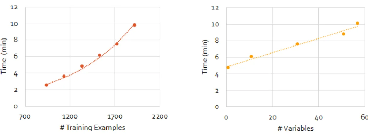
3.4. Computation time management ... 35

4. Results ... 40

4.1. Forecasting models results ... 40

4.2. Comparison of forecasting methods ... 42

4.2.1. Present information scenario ... 42

4.2.2. Adding Past Information ... 44

4.2.3. ν-SVR ... 47

5. Conclusions ... 49 6. References ... 51

Figures and Table Index

Figure 1.1: PV Installations evolution along the years [2000-2016] [6] ... 15

Figure 1.2: Global Cumulative Residential PV Installations (GW) Source: IHS Markit predict 2017 [21] ... 17

Figure 1.3: Example of various residential PV systems with their location and generation know. The green bar indicates the PV electric production of each system and the wind direction is indicated by the grey arrow at the top right... 18

Figure 2.1: Forecast Process for Statistical Approach [33] ... 21

Figure 2.2: Common Kernels [45] ... 25

Figure 2.3: On the left the representation for three different system and on the right the K index result ... 27

Figure 3.1: Location and Distance Representation of the Data Systems ... 31

Figure 3.2: Process of Selection of days for Training, Validation, and Testing ... 32

Figure 3.3: Process rearranged for no Validation Set ... 33

Figure 3.4: ε-SVR time distribution ... 36

Figure 3.5: Order of Selection for the Systems to be studied ... 36

Figure 3.6: Representation of the Systems Chosen ... 37

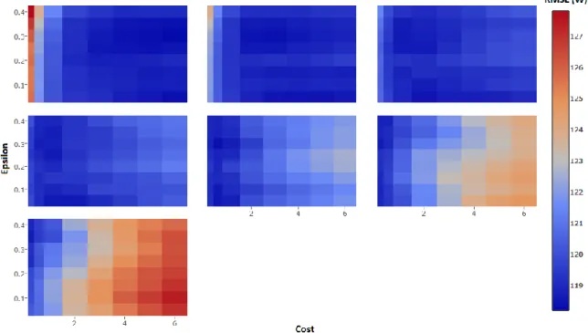
Figure 3.7: Results for a different cost, epsilon and gammas combinations. Each plot is a new gamma. Best RMSE Station ... 37

Figure 3.8: Results for a different cost, epsilon and gammas combinations. Each plot is a new gamma. Medium RMSE Station ... 38

Figure 3.9: Results for a different cost, epsilon and gammas combinations. Each plot is a new gamma. Worst RMSE Station ... 38

Figure 4.1: PV reading [black line] vs Forecast PV [colour line] for 5 days (Horizon =1, one random individual system) ... 40

Figure 4.2: PV reading [black line] vs Forecast PV [colour line] for 5 days (Horizon =6, one random individual system) ... 41

Figure 4.3: PV reading [black line] vs Forecast PV [colour line] for 5 days (Horizon =1, Regional system) ... 41

Figure 4.4: PV reading [black line] vs Forecast PV [colour line] for 5 days (Horizon =6, Regional system) ... 42

Figure 4.5: BIAS Results (Left: Individual System, Right: Regional System) Note: The areas shown in the left plot correspond to the ranges for each model considering the highest and lowest system’s BIAS value ... 42

Figure 4.6: MAE Results (Left: Individual System, Right: Regional System) Note: The areas shown in the left plot correspond to the ranges for each model considering the highest and lowest system’s MAE value ... 43 Figure 4.7: RMSE Results (Left: Individual System, Right: Regional System) Note: The areas shown in the left plot correspond to the ranges for each model considering the highest and lowest

Figure 4.8: Forecasting Skill [%] (Left: Individual System, Right: Regional System) Note: The areas shown in the left plot correspond to the ranges for each model considering the highest and

lowest system’s Skill value ... 44

Figure 4.9: Adding Azimuth and Solar Angle (Left: Individual System, Right: Regional System) . 44 Figure 4.10: Results for Skill [%] with n=3 (top) and n=5 (below) (Left: Individual System, Right: Regional System) Note: The areas shown in the left plot correspond to the ranges for each model considering the highest and lowest system’s Skill value... 45

Figure 4.11: Results for nRMSE [%] for n=3 (top) n=5 (below) ((Left: Individual System, Right: Regional System) Note: The areas shown in the left plot correspond to the ranges for each model considering the highest and lowest system’s nRMSE value ... 46

Figure 4.12: Number of points forecasted in the test set for every model ... 46

Figure 4.13: Results of Skill [%] using different nu to the ϵ-SVR counterpart (Left: Individual System, Right: A cumulative System) Note: The individual case stain range of each model is the interval between the highest and lowest system’s Skill value ... 47

Figure 4.14: Results of nRMSE [%] using different nu to the ϵ-SVR counterpart (Left: Individual System, Right: A cumulative System) Note: The individual case stain range of each model is the interval between the highest and lowest system’s nRMSE value ... 47

Table 3.1: Kernels Available ... 34

Table 3.2: Parameters used for SVR ... 34

Symbology

PV Photovoltaic

DSO Distribution System Operator

TSO Transmission System Operator

DG Distributed Generation

NWP Numerical Weather Prediction

NWS National Weather Service

GHI Global Horizontal Irradiance

SAM System Advisor Model

IDE Integrated Development Environment

CRAN Comprehensive R Archive Network

PPF Past Predicts Future model

NN Neural Network

AR Auto Regressive

ARMA Auto-Regressive Moving Average

ARIMA Auto-Regressive Integrated Moving Average

ARX Multiple Linear Regression

SVM Support Vector Machine

SVR Support Vector Regression

WSVM Weighted Support Vector Machine

MSE Mean Square Error

RMSE Root Mean Square Error

nRMSE Normalized Root Mean Square Error

MAE Mean Absolute Error

NA Missing Values W Watt kW Kilowatt MW Megawatt GW Gigawatt kWh Kilowatt hour

kVAh Kilo-volt-ampere hour

1.

Introduction

This chapter makes a brief introduction to the photovoltaic topic and the motivation for the use of forecasting techniques by system operators (mainly focused on the distributed system operator) for photovoltaic production. The objectives and organization of this work are also presented.

1.1. Context

In presents days, we get approximately 80% of the energy we consume from non-renewable energy sources, e.g. fossil fuels [1]. The increase in emissions of greenhouse gases and pollutants is correlated with the conversion of fossil fuels to electricity, heat, and transport. This leads to global warming that disturbs the delicate ecosystems and could easily relegate many species to extinction [2]. To prevent a global warming calamity, the global temperature should be kept to or around 1.5 ºC above pre-industrial temperatures. For this target, the global greenhouse gas emissions should be reduced worldwide to approximately 80% from their 1990 levels, by 2050 [3].

Utilizing renewable sources energy such as wind and solar to generate electricity provides a feasible contribution for the greenhouse gas reduction challenge as these are emission-free sources of energy that can be used to generate electricity and at the same time protect our environment for future generations.

Solar energy, in particular photovoltaic (PV), can fulfill all the electricity needs of humankind [4]. In the last decade, PV solar energy has started realizing its huge potential, as the amount of installed PV power is rapidly increased, also with the integration of solar cells into the roofs and facades of buildings [5].

After a limited development in 2014, the market restarted its fast growth, almost everywhere, with all regions of the world contributing to PV development for the first time. In 2015, the PV market broke several records and continued its global expansion, with a 25% growth at 50 GW. The total installed capacity at the end of 2015 globally amounted to at least 227 GW, ten times higher than in 2009. In 2016, the worldwide PV market showed again a great potential, breaking again several records and continuing with its global expansion, with a 50% increase [4].

Overall, these developments raised the annual global PV market to at least 75 GW, with a positive outcome in all regions of the world. Photovoltaic has now reached 1 GW of regional penetration on all continents, much more on the leading ones (Asia, Europe, and North America). The total global installed capacity as passed the 300 GW mark, as shown in Figure 1.1 [6].

The increase in the capacity installed yearly has been coupled with a strong decrease in the components price. Since 2006, the PV system price has shown a reduction of more than 50%, e.g. the standard final price in 2006 was around 5500-6000 €/kW for a residential system, whereas in 2017 the standard final price was approximal 2400-2700 €/kW [5].

Figure 1.1: PV Installations evolution along the years [2000-2016] [6]

It was thought that integrating PV systems into electrical grids would not be a difficult task; however, when the penetration level of PV systems started to increase, utilities began to face new non-traditional challenges mainly due to the discontinuous nature of solar energy [7]. Photovoltaic array output is highly dependent on environmental conditions such as illumination intensity and temperature. For example, the presence of clouds or high wind velocity can reduce the power output of solar cells and the presence of dust on the surface of the solar panels deteriorates their performances [8]. Thus, the power system must deal with not only uncontrollable demand but also uncontrollable generation [9].

Photovoltaic systems can impose negatives impacts on the electrical grid, dependent on the size as well as the location of the PV system. They may be classified based on their ratings into three different categories: i) Small systems rated as 10 kW and less, ii) intermediate PV systems rated from 10 kW to 500 kW and iii) large PV systems rated above 500 kW. The first two categories are usually managed by the distribution system operator (DSO) and the latter by the transmission system operator (TSO) [10].

Some of the main negative impacts of PV systems on the DSO side are as follows:

Reverse Power Flow

In the distribution system, the power flow is usually unidirectional from the Medium Voltage system to the Low Voltage system. However, at a high penetration level of PV systems, there are moments when the net production is higher than the net demand, especially at noon. As a result, the direction of power flow is reversed, and power flows from the Low Voltage side to the Medium Voltage side. This reverse power flow results in overloading of the distribution feeders and excessive power losses. The reverse flow of power has also been reported to affect the operation of automatic voltage regulators installed along distribution feeders as the settings of such devices need to be changed to accommodate the shift in load center [11].

Utilities can mitigate this adversity by setting a limitation to the PV power to be exported or simply blocking the export since the PV power is typically used for local loads. If a frequent accurate forecast of PV power could be done these limitations could be controlled relatively well [12].

Power Losses

Distributed Generation (DG) systems, in general, reduce system losses as they bring generation closer to the load. This assumption is true until reverse power flow starts to occur.

Miller and Ye showed that distribution systems losses reach a minimum value at a penetration level of approximately 5% but losses increases as the penetration level increases [13]. So, a key challenge is managing reverse power flow from happening.

Voltage Control Difficulty

In a power system with embedded generation, voltage control becomes a difficult task due to the existence of more than one supply point, in this case, will appear situations of overvoltage and under voltage [14].

As an example, the PV output is high when it is sunny, but when clouds appear PV output power can drop very quickly resulting in an under-voltage condition. This problem can be mitigated using weather prediction to reduce the expected amount of output power when clouds are expected. This requires the use of real-time weather measurements and weather forecast algorithms [15].

Increased Reactive Power

Photovoltaics system inverters normally operate at unity power factor for two reasons. The first reason is that standards do not allow PV system inverter to operate in voltage regulation mode. The second reason is that owners of small residential PV systems normally are paid for their kWh yield, not their kVAh production. Thus, they prefer to operate their inverters at unity power factor to maximize the active power generated and accordingly, their return. As a result, the active power requirements of existing loads are partially met by PV systems, reducing the active power supply from the utility. However, the reactive power requirements are still the same and must be supplied completely by the utility. A high rate of the reactive power supply is not preferred by the utilities because in this case distribution transformers will operate at very low power factor and the efficiency of transformers decreases as their operating power factor decreases. Hence overall losses in distribution transformers will increase reducing the overall system efficiency [16].

Islanding

It is necessary to detect when the system operates in an island mode and to disconnect it from the grid as soon as possible. The island can occur when a part of the grid is electrically isolated from the power system but the part with island is energized by distributed generators. The islanding detection is important for many reasons - a possibility to damage customer equipment’s and distributed generator, hazard for line-workers, islanding may interfere with restoration of normal services for neighboring customers [17].

For a quality and reliable distribution of power produced by PV systems the ability of precise forecast the energy produced is of great importance and has been identified as one of the key challenges for massive integration [18].

1.2. Motivation

Solar forecasting provides a way for system operators to predict and balance energy generation and consumption. Assuming the system operator has a mix of generating assets at their disposal, reliable solar forecasting allows optimization of dispatch their controllable units. Thus, a proper PV forecast would be able to lower the number of units in hot standby and, consequently, reduce the operating costs.

In this perspective, an inaccurate solar forecast means a need to make up for unpredicted imbalance with shorter-term sources of power. These short-term sources tend to be costlier on a per unit basis, which also means that the extent of total inaccuracy is important. For instance, the total cost to make up a 10% error on a 10 MW and 100 MW plant will, of course, be very different. This cost can then be passed through from the system operator to the market participants.

These types of penalties have existed with controllable generation to assure reliable power delivery to the grid operator but are now becoming an option for renewable plant operators that see economic value in using forecasts to schedule power. Accurate forecasting is required to take on that type of additional risk. So, an accurate forecast is not only beneficial for system operators since it reduces costs and uncertainties, but also for PV plant managers, as they avoid possible penalties that are incurred due to deviations between forecasted and produced energy [19].

From all renewable sources explored in Portugal, PV technology saw the largest relative increase in installed capacity, going from practically inexistent in 2006 to 467 MW in the end of 2016, is approximately 72 MW in the residential sector [20]. This residential growth tendency can be seen in Europe and in the rest of the world, and the tendency is to continue to go up Figure 1.2.

Figure 1.2: Global Cumulative Residential PV Installations (GW) Source: IHS Markit predict 2017 [21]

This residential growth can be attributed mainly due to the reduction in the price of PV systems components, with a focus on batteries, and incentive politics that are done in each country. Even so, the prices for the majority of the population is too high [22].

Given the increasing number of installed small PV systems, new challenges regarding the grid integration of PV generated electricity is coming up. Amongst those challenges is the issue of ramps and peaks of the injected PV power into low voltage grids, as talked in the context topic.

In this new challenge resides the main motivation for the DSO side, being the main objective of this perspective maintain the quality of energy (tension and safety of distribution) and managing the electric network with efficiency, to reduce losses. If the DSO can’t guarantee the quality of energy distributed, they need to compensate the customers and the overutilization of the electrical network assets will impact its lifespan. The other barrier is how efficiently the network can be handled since if it is badly managed it will impact directly on the operational cost. Forecasting the

PV power production would help mitigate this problem and create new solutions for load control [23].

Either way, the trustworthy forecasting of the expected PV power production is crucial for the integration of high shares into our energy system

1.3. Objectives

With the increase of PV distributed generation, the necessity to forecast their power output is growing necessity for the DSO operations. So, the main objective of this dissertation is to study and develop a forecasting model for solar PV distributed generation with the perspective of the DSO, responsible for operating, ensuring the maintenance of and, if necessary, developing the distribution system in each area.

The various systems will be analyzed as a black box, with the purpose that the forecasting model can be applied to any system without knowing their technical details. The information available will be the installed power, the location and the historical generation of each system, Figure 1.3 represents an example of this condition. In this example we can see that the systems closer to the clouds are producing less than the system further away, in this manner if the historical data for the generation of each system and their distance could be used in the forecasting model, it could interpret the movement of the clouds, improving the forecast accuracy.

Figure 1.3: Example of various residential PV systems with their location and generation know. The green bar indicates the PV electric production of each system and the wind direction is indicated by the grey arrow at the top right.

Nowadays there is a great variety of forecasting techniques so developing all of them would have been too time and computationally demanding, so with the interest of time and work management three techniques were chosen, Persistence (as a base model for comparison), Multivariable Regression (as a simple and efficient model) and Support Vector Regression (more advanced model with the potential of having superior performances).

1.4. Organization of the dissertation

This chapter introduced the impacts and challenges of large-scale integration of photovoltaics in the grid, the motivation of the work and defining its objectives.

In chapter two the different models used for this work are presented. It is described how forecast methods work in general and a theoretical explanation of each model used, their process, variables, advantages, and disadvantages.

Chapter three is devoted to the methodology used in this work. Knowing that the models had already been used and studied, the objective is not to focus directly on the model but rather how the models react to different variables with an index in forecasting decentralized PV power with a peer-to-peer information.

In chapter four the results and their interpretations are presented, for each figure will be pointed out the analyzes, the test carried out and discussion of the results obtained.

2.

Solar forecasting

This chapter presents the state of the art of solar forecasting techniques used in this dissertation, persistence, multivariable and support vector regressions, together with a brief explanation of models that use PV power as an index for PV forecast.

2.1. Overview

Accurate power prediction can enhance the stability and security level and lead to a more economical operating decision for the power system. Due to meteorological uncertainty, PV energy is difficult to predict. Weather variables such as temperature, global solar irradiation, sunshine duration, wind speed, relative humidity, cloudiness/sky cover, precipitation and dew point are used as inputs for solar power forecasting models. Solar irradiation varies with time, season, geographical location and meteorological conditions [24]. Since the output power of a solar panel at a fixed temperature is closely linear dependent of the global irradiance [25], predicting solar irradiance is not expected to be very different from predicting PV power, at least in a first approach.

The choice of a model depends on the forecasted horizon, tools, data available, required resolution, accuracy, and purpose. In general, forecasting may be distinguished according to the horizon time scale,but there is no consensus in the literature as to what the thresholds should be. One possible classification [26] is as follows:

Very short-term generally involves horizons from a few seconds up to a few hours ahead. These services are important for grid operators to guarantee grid stability.

Short term from a few days to a few months ahead. They are useful in daily operations of utility companies and valuable for electric market operators [27]. Forecasting the power output of a PV pant for the next few hours or days is necessary for the optimal integration in the electric network.

Long-term with lead times measured in months, quarters or even years. The long-term forecast is necessary for strategic planning. Their information is essential for capacity expansion, capital investment decisions, revenue analysis and corporate budgeting [28], [29].

2.2. Forecasting Models

Forecasting methods can be broadly characterized as physical or statistical [30]. Physical models are based on mathematical equations which describe physical state and dynamic motion of the atmosphere. This approach uses different weather forecasts such as global horizontal irradiance, ambient temperature, relative humidity, wind speed and PV system characteristics such as system location, orientation and historical data or manufacturer specification as inputs of solar and PV models which perform forecast of irradiation in an array plane and back of module temperature [31], [32].

In the statistical approach historical data of PV power and various inputs, such as a ground station or satellite data, numerical weather prediction (NWP) outputs and PV system data are used. A historical dataset is chosen to train a model and to determine unknown model parameters. Models output a forecast of PV power at a given time based on past inputs proceeded by analysis, Figure 2.1.

Figure 2.1: Forecast Process for Statistical Approach [33]

A few key components make up solar forecasting tools. First, there is the weather model. As mentioned above, solar generation is variable by nature. Cloud cover causes this variability by obstructing sunlight from hitting the solar panels. If one can predict the weather with a great amount of certainty, one is already one step ahead of improving our forecast.

The second factor in a solar forecast is the model used to convert the weather into system power output. The solar industry uses these “PV simulation” models to predict the performance of a PV system under environmental conditions like irradiance, wind speed, temperature and relative humidity. PV simulation models may also incorporate important PV systems behaviors such as tracking, which predicts the orientation of the PV panels mounted on single- or dual-axis tracking hardware.

Some of the main statistical analysis methods used in power generation forecasting are multiple linear regressions [34], neural networks (NN) [35], support vector machines (SVM) [36], autoregressive moving average (ARMA) [37], autoregressive integrated moving average (ARIMA) [38] for non-stationary time-series.

2.2.1. Persistence

Some simple forecast techniques can serve as benchmarks that can be used to evaluate forecast improvements. One very simple and commonly used reference is the Persistence method. The Persistence model as shown results that can outperform the NWP models, the reason for this is that it can inherit a better representation of the temperature effects on the panels that are not present as an input to the GHI (Global Horizontal Irradiance) to the power output a day-head model [39]. The error in the Persistence increases considerably as the hour-ahead increases, as such the Persistence model is only suitable for very short term forecasting [40].

This method main idea sets that the conditions at the time of the forecast will not change, “things stay the same”, for example projecting past values of PV production into the future [4].

2.2.2. Multivariable Regression

Linear regression attempts to model the relationship between two variables by fitting a linear equation to observed data. One variable is known as the independent variables (X), and the other is often called the response variable (Y), being B0 the bias and B the model coefficients, equation

(2.1).

The overall idea of regression is to examine two things: (a) does a set of predictor variables do a good job in predicting an outcome variable? (b) Is the model using the predictors accounting for the variability in the changes in the dependent variable? [41].

These regressions are commonly used because they are the simplest and easiest non-trivial relationships to work with, in the majority of the case the key relationships between our variables are often or at least approximately linear over the range of values that are of interest to us and even if they are not, we can often transform the variables in such a way as to linearize the relationships [42].

The multivariable regression is very similar to a linear regression, the difference is in the number of variables we give the model, where we can have multiples explanatory variables, equation (2.2).

𝑌 = 𝐵0+ 𝐵1. 𝑋1+ 𝐵2. 𝑋2+ ⋯ + 𝐵𝑛. 𝑋𝑛 (2.2)

Multivariable linear regression analysis has three major uses. First, it can be used to identify the strength of the effect that the independent variables have on the dependent variable. Second, it can be used to forecast effects or impacts of changes, in other words, helps us to understand how much the dependent variable will change when we change the independent variables. Third, this model analysis predicts trends and future values that can be used to get point estimates.

When selecting the model, an important consideration is the model fit. Adding independent variables to multiple linear regression models will always increase the amount of explained variance in the dependent variable (typically expressed as R²). Therefore, adding too many independent variables without any theoretical justification may result in an over-fit model [41].

When the spatial information is an important variable, auto-regressive (AR) regression can be proven very useful. Overall the auto-regressive model specifies that the output variable will depend linearly on its own previous value and a stochastic term (an imperfectly predictable term). The main advantage of the AR is that the model explicitly accounts for autocorrelation in the error allowing for a valid inference to be made, while normal linear regression assumes uncorrelated errors, with autocorrelated data, this assumption fails and so inference drawn from the regression model will be invalid (standard error, etc)[43].

2.2.3. Support Vector Regression

Support vector machines were, initially, a learning algorithm orientated for linear problems of classification, where they would separate two linear classes in a hyperplane. Later it was proposed for non-linear problems, mapping of points in one space and projecting it for a bigger dimension space, where they are divided according to the class to which they belong, with the intention of maximizing the separation margin. After this, the notion of Support Vector Regression (SVR) was introduced, a generalization of SVM for regression problems (Vapnik, 1995) [36], one of the main advantage of this method is that it can capture the nonlinearity in a dataset.

For a brief explanation of the SVR equations, let's assume that we are given training data {(𝑥1, 𝑦1), … , ( 𝑥𝑙, 𝑦𝑙 )} )} ⊂ ℵ × ℜ, where ℵ represents the space of the inputs patterns – for

instance ℜ𝑑. In ε-SVR the objective has been to find a function f(x) that has at most ε deviation from the obtained targets 𝑦𝑖 for all the training data and at the same time as flat as possible. For the

where 〈… 〉 stand for the dot product in ℵ. Flatness in (2.3) means small 𝜔. For this, it is required to minimize its Euclidean norm i.e. ‖𝜔‖2. Regularly this can be written as a convex optimization problem by requiring 𝑚𝑖𝑛𝑖𝑚𝑖𝑧𝑒 1 2‖𝜔‖ 2 _(2.4) 𝑠𝑢𝑏𝑗𝑒𝑐𝑡 𝑡𝑜 { 𝑦𝑖− 〈𝜔, 𝑥𝑖〉 − 𝑏 ≤ 𝜀 〈𝜔, 𝑥𝑖〉 + 𝑏 − 𝑦𝑖 ≤ 𝜀 (2.5)

The above convex optimization problem is achievable in cases where f exists and approximates all pairs (𝑥𝑖, 𝑦𝑖) with 𝜀 precision. Introducing slack variables 𝜉𝑖 , 𝜉𝑖∗ (slack variable is a variable that is

added to an inequality constraint to transform it into an equality) to cope with the constraints of the optimization problem, (2.4) and (2.5), the formulation becomes

𝑚𝑖𝑛𝑖𝑚𝑖𝑧𝑒 1 2‖𝜔‖ 2_{+ 𝐶 ∑(𝜉} 𝑖 + 𝜉𝑖∗) 𝑙 𝑖=1 (2.6) 𝑠𝑢𝑏𝑗𝑒𝑐𝑡 𝑡𝑜 { 𝑦𝑖− 〈𝜔, 𝑥𝑖〉 − 𝑏 = 𝜀 + 𝜉𝑖 〈𝜔, 𝑥_𝑖〉 + 𝑏 − 𝑦_𝑖 = 𝜀 + 𝜉𝑖∗ 𝜉𝑖 , 𝜉𝑖∗≥ 0 (2.7)

The constant C > 0 determines the trade-off between the flatness of f and the amount up to which deviations larger than 𝜀 are tolerated. 𝜀-insensitive loss function, |𝜉|𝜀 has been described by

|𝜉|_𝜀 = {_{|𝜉| − 𝜀 𝑜𝑡ℎ𝑒𝑟𝑤𝑖𝑠𝑒}0 if |𝜉| < 𝜀 (2.8) The dual formulation provides the key for extending SVM to nonlinear functions. The standard dualization method utilizing Lagrange multipliers has been described as follows:

𝐿 = 1 2‖𝜔‖ 2_{+ 𝐶 ∑(𝜉} 𝑖 + 𝜉𝑖∗) 𝑙 𝑖=1 − ∑ 𝛼𝑖(𝜀 + 𝜉𝑖 − 𝑦𝑖+ 〈𝜔, 𝑥𝑖〉 + 𝑏) 𝑙 𝑖=1 − ∑ 𝛼𝑖∗(𝜀 + 𝜉𝑖∗ + 𝑦𝑖− 〈𝜔, 𝑥𝑖〉 − 𝑏) 𝑙 𝑖=1 − ∑(𝜂𝑖𝜉𝑖+ 𝜂𝑖∗𝜉𝑖∗) 𝑙 𝑖=1 (2.9)

The dual variables in equation (2.9) must satisfy positivity constraints i.e. 𝛼𝑖, 𝛼𝑖∗, 𝜂𝑖, 𝜂𝑖∗ ≥ 0. It

follows from saddle point condition that the partial derivatives of L with respect to the primal variables (𝜔, b, 𝜉𝑖, 𝜉𝑖∗) should vanish for optimization.

𝜕𝐿 𝜕𝑏= ∑( 𝑙 𝑖=1 𝛼_𝑖∗− 𝛼𝑖) = 0 (2.10) 𝜕𝐿 𝜕𝜔= 𝜔 − ∑( 𝑙 𝑖=1 𝛼_𝑖∗− 𝛼𝑖)𝑥𝑖= 0 (2.11) 𝜕𝐿 𝜕𝜉_𝑖∗= 𝐶 − 𝛼𝑖 ∗_{− 𝜂} 𝑖 ∗_{= 0 (2.12)}

Substituting equation (2.10)(2.11)(2.12) into (2.9) yields the dual optimization problem. 𝑀𝑎𝑥𝑖𝑚𝑖𝑧𝑒 {−1 2 ∑ (𝛼𝑖− 𝛼𝑖 ∗_)(𝛼 𝑗− 𝛼𝑗∗) 𝑖,𝑗=1 〈𝑥_𝑖, 𝑥𝑗〉 − 𝜀 ∑(𝛼𝑖− 𝛼𝑖∗) + ∑(𝛼𝑖− 𝛼𝑖∗) 𝑙 𝑖=1 𝑙 𝑖=1 } (2.13) 𝑆𝑢𝑏𝑗𝑒𝑐𝑡 𝑡𝑜 ∑(𝛼𝑖− 𝛼𝑖∗) 𝑙 𝑖=1 = 0 𝑎𝑛𝑑 𝛼𝑖, 𝛼𝑖∗∈ [0, 𝐶] (2.14)

Dual variables 𝜂𝑖, 𝜂𝑖∗ trough condition (2.13) have been eliminated for deriving (2.14). As

consequence (2.11) can be rewritten as follow:

𝜔 = ∑(

𝑙

𝑖=1

𝛼𝑖− 𝛼𝑖∗)𝑥𝑖 (2.15)

and therefore from Eq. (2.3) 𝑓(𝑥) = ∑(

𝑙

𝑖=1

𝛼𝑖− 𝛼𝑖∗)〈𝑥𝑖, 𝑥〉 + 𝑏 (2.16)

This is named support vector expansion i.e. 𝜔 can be completely described as a linear combination of the training patterns xi. Notice that 𝜔 does not have to be computed explicitly, even for

evaluating f(x).

Computation of b is done by exploiting Karush-Kuhn-Tucker (KKT) conditions [36] which states that at the optimal solution the product between dual variables and constraints must vanish. In this model, means that:

𝛼𝑖(𝜀 + 𝜉𝑖− 𝑦𝑖+ 〈𝑤, 𝑥𝑖〉 + 𝑏) = 0 (2.17) 𝛼𝑖∗(𝜀 + 𝜉𝑖∗− 𝑦𝑖+ 〈𝑤, 𝑥𝑖〉 + 𝑏) = 0 (2.18) and (𝐶 − 𝛼𝑖)𝜉𝑖 = 0 (2.19) (𝐶 − 𝛼_𝑖∗_)𝜉 𝑖∗= 0 (2.20)

Following this reasoning, only samples (𝑥𝑖, 𝑦𝑖) with corresponding 𝛼𝑖∗= 𝐶 lie outside the

ε-insensitive tube around f and 𝛼𝑖𝛼𝑖∗= 0, i.e. there can never be a set of dual variables 𝛼𝑖𝛼𝑖∗ which

are both simultaneously nonzero as this would require nonzero slacks in both directions. Finally, for 𝛼𝑖∗∈ (0, 𝐶), 𝜉𝑖∗= 0 and moreover the second factor in (2.17) and (2.18) need to vanish, hence b

can be computed as follows:

𝑏 = 𝑦𝑖− 〈𝜔, 𝑥𝑖〉 − 𝜀 𝑓𝑜𝑟 𝛼𝑖 ∈ (0, 𝐶) (2.21)

𝑏 = 𝑦𝑖− 〈𝜔, 𝑥𝑖∗〉 − 𝜀 𝑓𝑜𝑟 𝛼𝑖∗ ∈ (0, 𝐶) (2.22)

From (2.17) and (2.18), it follows that only for |𝑓(𝑥𝑖) − 𝑦𝑖| ≥ 𝜀 the Lagrange multipliers may be

nonzero, or in other words, for all samples inside the 𝜀-tube, the 𝛼𝑖, 𝛼𝑖∗ vanish for |𝑓(𝑥𝑖) − 𝑦𝑖| < 𝜀

the second factor in (2.17) and (2.18) is nonzero, hence 𝛼𝑖, 𝛼𝑖∗ has to be zero such that the KKT

conditions are satisfied. Therefore, a sparse expansion of 𝜔 exists in terms of xi (note: not all xi are

One important step is turning the SVR algorithm to nonlinear problems and this can be done simply by pre-processing the training patterns xi by a map 𝜙: 𝑋 → ℑ, into some feature space ℑ and then

applying the standard SVR algorithm. Then the expansion in (2.15) and (2.16) becomes:

𝜔 = ∑( 𝑙 𝑖=1 𝛼𝑖− 𝛼𝑖∗)𝜙(𝑥𝑖) (2.23) and therefore 𝑓(𝑥) = ∑( 𝑙 𝑖=1 𝛼𝑖− 𝛼𝑖∗)𝑘(𝑥𝑖, 𝑥) + 𝑏 (2.24)

The difference with the linear case is that 𝜔 is no longer explicitly given. In the nonlinear setting, the optimization problem corresponds to finding the flattest function in feature space, not in input space. The standard SVR to solve the approximation problem is as follows:

𝑓(𝑥) = ∑(

𝑁

𝑖=1

𝛼_𝑖∗− 𝛼𝑖)𝑘(𝑥𝑖, 𝑥) + 𝑏 (2.25)

the kernel function 𝑘(𝑥𝑖, 𝑥) has been defined as way to compute the dot products of two vectors 𝑥𝑖

and 𝑥 in some (possibly very high dimensional) feature space.

𝑘(𝑥𝑖, 𝑥) = 𝜑(𝑥𝑖)𝜑(𝑥) (2.26)

So instead of mapping our data via 𝜙 and computing the inner product, we can do it in one operation, leaving the mapping completely implicit. This "trick" is called the kernel trick. This process can be implemented so smoothly because of the optimization from the dual formulation and when testing a new example, we only need to sum over the support vectors which is much faster than summing over the entire training-set.

Unfortunately, choosing the 'correct' kernel is a nontrivial task, and may depend on the specific task at hand. No matter which kernel you choose, you will need to tune the kernel parameters to get good performance from your classifier. Popular parameter-tuning techniques include K-Fold Cross Validation [44]. The most used kernels are the polynomial, radial basis functions (RBF) and Saturating (sigmoid-like), Figure 2.2.

Figure 2.2: Common Kernels [45]

The Lagrange multipliers 𝛼𝑖∗ and 𝛼𝑖 of (2.25) have been obtained by minimizing the following

𝑅𝑟𝑒𝑔|𝑓| = 1 2‖𝜔‖ 2_{+ 𝐶 ∑ 𝐿} 𝑒(𝑦) 𝑙 𝑖=1 (2.27)

where the term ‖𝜔‖2 has been characterized as the model complexity, C as a constant determining the trade-off and the ε-insensitive loss function, 𝐿𝑒(𝑦) given by

𝐿𝑒(𝑦) = {

0, for |𝑓(𝑥) − 𝑦| < 𝜀

|𝑓(𝑥) − 𝑦| − 𝜀, 𝑜𝑡ℎ𝑒𝑟𝑤𝑖𝑠𝑒 (2.28) In classical support vector regression (ε-SVR), the proper value for the parameter ε is difficult to determine beforehand. Fortunately, this problem is partially resolved in the algorithm, ν support vector regression (ν-SVR), in which ε itself is a variable in the optimization process and is controlled by another new parameter ν ∈ [0,1]. ν is the upper bound on the fraction of error points or the lower bound on the fraction of points inside the ε-insensitive tube, allowing to determine the proportion of the number of support vectors, we desire to keep in our solution, with respect to the total number of samples in the dataset. Thus, a good ε can be automatically found by choosing ν, which adjusts the accuracy level to the data at hand. This makes ν a more convenient parameter than the one used in ε--SVR [46].

However, in ε-SVR you have no control over how many data vectors from the dataset become support vectors, it could be a few, it could be many. Nonetheless, you will have total control of how much error you will allow your model to have, and anything beyond the specified ε will be penalized in proportion to C, which is the regularization parameter.

2.2.4. Clear-sky Index

Solar radiation is always greater in an area that extends perpendicularly to the sunbeams, than in a horizontal area with the same dimensions. Because of earth’s rotation and this axis of rotation is tilted, the azimuth and the solar height change throughout the day and the year, the angle of incidence of the solar radiation constantly varies in the areas with the potential to the use of solar energy. In this manner obstacles to the sunlight can have different impacts according to the time of the year, as an example the radiation from a clear-sky mid-day in winter can have the same solar radiation value as a cloudy morning in the summer [47]. As such some of the major challenging factors for PV forecasting are the orientation/inclination of the system since different positions result in different solar profiles and the possible presence of obstacles which provoke shades, originating drastic power variations.

One way to approach this problem would be normalizing radiation measurements to their clearness index, firstly done by J. N. Black, [48]. In this work, the ratio between the daily radiation measurements and they theoretical counterparts in a perfectly transparent atmosphere, called “clearness index”, was used to develop regression equations for forecasting daily radiation from sunshine hour observations.

The usefulness of this index was reinforced some years after by B. Y. H. Liu and R. C. Jordan [49], for estimating the performance of tilted flat-plate solar collectors. The methods used before this study needed a detailed record of the radiation and temperature data of the locality of the collector. The fact that a large volume of meteorological radiation and temperature data must be analyzed made the prediction of collector performance an extremely tedious and time-consuming task. The work done in this study made this process easier. They used generalized φ-curve (based in various

collector of any angle or tilt at any locality can be predicted when the following two parameters are known: the monthly-average daily total radiation on a horizontal surface and the monthly-average day-time ambient temperature.

A further technique of the clearness index concept has become possible since the development of proficient clear-sky radiation modeling (e.g. Golnas 2011, [50]). By modeling the clear-sky radiation arriving at the surface of the Earth, the denominator of the clearness index (previously the extra-terrestrial component of irradiance) can be replaced with this clear-sky estimate, thereby changing it to the well-known “clear-sky index” which most modern methods now utilize, equation (2.29). This index is a dimensionless number between 0 and 1, has a high value under clear, sunny conditions, and a low value under cloudy conditions.

𝐾𝑖𝑛𝑑𝑒𝑥=

𝑀𝑒𝑎𝑠𝑢𝑟𝑒𝑑

𝐶𝑙𝑒𝑎𝑟 𝑆𝑘𝑦 𝑒𝑠𝑡𝑖𝑚𝑎𝑡𝑒 (2.29)

This model, as handy it can be to calculate the irradiation the system receives, the transition from irradiance to power is not trivial since it implies knowing other variables as, module temperature, inverter efficiency, model efficiency, etc. If these variables are known, models like the one proposed by N. Engerer and F.P.Mills, [51], that uses a horizontal clear-sky radiation model, transposes and then converts to PV power with physical equations, can be a great choice.

A rather different approach is that of Lonij [52] or Bacher [53], that uses a statistic way, in their index, instead of applying to global irradiance it is applied on solar power. In this manner, the application of the clear-sky index to PV power was simplified, and both cases presented interesting forecasting results.

An example where the importance of estimating the clear-sky index is illustrated in Figure 2.3. It is shown that this index ignores changes in the day of the year or system positioning and can also isolate the cloud-induced variability.

2.3. Studies Overview

Achieving high accuracy forecasts at each time scale imposes specific requirements to the applicable data sources, solar irradiation models, and forecasting techniques converting available data into quality solar power forecasts [29].

Kostylev and Pavlovski, [29], also Huang, [40], describe forecasting methods depending on the tools and information available to forecasters. This includes PV system data, proprietary models such as total sky image based or satellite-based cloud cover and irradiation forecasts and publicly available results NWP models.

Kostylev and Pavlovski [29] states that forecast accuracy strongly depends on the climatic conditions at the forecast site since the cloud regime strongly defines the success of the forecast performance. The example given is from Central European stations, the relative root mean square error (RMSE) ranged from 40% to 60% (% of mean observed), while for sunnier Spanish stations relative RMSE values were in the range of 20% to 35%.

Huang, [40], results demonstrate that the ARMA model is suitable for short and medium term forecasting and the Persistence have good results in short previsions. The ARMA procedure includes obtaining the historical solar radiation data from SolarAnywhere and using System Advisor Model (SAM) for the historical solar generation data. The maximum mean square error (MSE) for the ARMA model was 0.028 kW (in March), showing improvements over of the persistence of 44.38% (in January), this was done for forecasting of 1-hour ahead horizon for a laboratory-level micro-grid scenario.

Elke [30] describe and evaluate the approach of irradiance forecasting, which is the basis for PV power prediction. They present an approach to derive weather specific prediction intervals for irradiance forecasts. First, site-specific hourly forecasts are derived from the low-resolution forecasts of the European Centre for Medium-Range Weather Forecasts. In a second step, the forecast of the global horizontal irradiance must be converted to the module plane with a tilted irradiance model. Finally, the power output forecast is obtained by applying a PV simulation model to the forecasted irradiance. The model returns the alternating current power feed to the grid as a function of the incoming irradiance and the ambient temperature. They showed that the forecast errors are smaller than 5% of the nominal power in more than 80% of all situations and smaller than 10% of the nominal power in more than 90% of all situations.

Sharma [54] study developed prediction models using historical NWS (National Weather Service) forecast data and correlated them with generation data from solar panels. Their analysis quantifies how each forecast parameter affects the other and the solar intensity. For solar energy harvesting, they found that sky cover, relative humidity, and precipitation is highly correlated with each other and with solar intensity, while temperature, dew point, and wind speed are only partially correlated with each other and with solar intensity. They studied how solar intensity varies with individual forecast parameters and how these forecast parameters are related to each other. They also showed how a day of a year affects solar intensity. For this, they used linear least squares and SVM using multiple kernel functions. Their results concluded that the RMSE for SVM-RBF with four dimensions is 128 W/m2_{, while the RMSE for cloudy and past predicts future model (PPF) is 175}

and 261 W/m2_{, respectively. Thus, SVM-RBF with four dimensions is 27% more accurate than the}

simple cloudy model and 51% more accurate than the PPF model.

weather databases including the global irradiance, and temperature using a data acquisition system. They present three forecasting models using simple regression and neural network methods based on artificial intelligence.

The study done by Xu and co-workers [56] adopts a weighted SVM to forecast the short-term PV power. They selected the five most similar days to the day to be forecasted as the training samples. The weights of the samples for the weighted Supported Vector Machine (WSVM) are designed based on similarities and the time point. The solar irradiation and the temperature were considered as the two main factors in the process of PV power forecasting. Therefore, a history of data including solar irradiation, temperature, and the output power was used to find the similar days. Increasing the number of similar days decreased the prediction accuracy other than improving it. In this work, they also used artificial NN to compare methods. The result showed that WSVM had a maximum of relative error of 12.23% versus the NN maximum relative error of 32.18% (the relative error here is the ratio of Mean Absolute Error (MAE) to the real value), being WSVM with a much smaller error than NN.

Another important feature for forecasting models is the information given to the training set, Kariniotakis and co-authors [57] showed that the accuracy increases with the training period size. Since the model can detect more patterns and relationships between the information provided and thus the model can have a better calibration. The near-optimal performance was reached with a training period of about 20 days. This procedure was done for the Random Forest model to a 200 kWp plant located in the south-east of France. The results had values around 10% RMSE (been normalized by the solar plant nominal power)

Pelland and co-authors [4] report on a general analysis of the state of the art of forecasting techniques, and states that the best day-ahead solar and PV forecasts combine NWP forecasts with postprocessing of these forecasts to improve them or to generate forecasts that are not included in the direct model outputs of the NWP, such as PV forecasts. Key post-processing approaches are a spatial-temporal interpolation, smoothing, and model output statistics. Also, it describes an example of non-parametric statistical methods (Random Forest and SVM) application to data obtained from a real, grid-connected PV power station located in France, demonstrating that these models managed to properly predict sunny days up to a satisfactory accuracy degree, whereas cloudy or unstable days pose more difficulties to be forecast. It his highlighted that the overall performance obtained is twice better than the typical performance for the case of wind farms at flat terrain.

With the increasingly centralized and decentralized PV generation, the more important is to know how to handle this variable source of energy production. Obtaining good forecasting performances is of a great help in handling this challenge since it can provide the information needed to control and maintain a trustworthy use of this energy in our grid as the economic implications it may have. The results obtained in various studies are promising but still not enough for a mass implementation, for this, the research done to forecasting topic is increasing and developing each year with slow but steady progress.

This work will be focused on developing some of the forecasting techniques already used, mainly SVR, using the clear sky index model in Lonij ([52]) with the extra condition that the system technical information is unknown but using the neighbors as a source of information for the model (a peer-to-peer approach). As such the next chapter will explain the process used to develop this approach.

3.

Methods

Three different forecasting models were developed: Persistence, Multivariable Regression (ARX) and SVR. The models were implemented in R (an open-source programming language) with the clear sky model. This chapter presents the details of the different methods, describes how they were implemented and how the quality of the outputs was assessed.

3.1. Data

The data used for testing and construction of the R script was originated from a region in the United Kingdom. These data contained the information from one year of PV production with a step of 30 min between each reading, beginning in the day 01/07/2015 to the end of the day 30/06/2016.

A brief analysis revealed that there are stations with a lot of missing values (NA) in certain months and the PV production was the accumulated value over the year. Stations with NAs were removed, giving the option to work with a full complete year of readings and the accumulated value was uncompressed getting the production at given time.

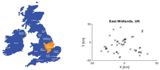
After these filters, the data to work with was that of 57 stations, represented in Figure 3.1. These stations were used as input variables in each model for the forecast of each individual stations.

Figure 3.1: Location and Distance Representation of the Data Systems

In the cases of machine learning algorithms, a computational model is trained to predict a certain unknown output. This training uses a target function represented by a finite set of training examples of inputs and the corresponding desired outputs. At the end of this process, the model should be able to predict correct outputs from their input as well be able to generalize to previously unseen data. Poor generalization can be characterized by over-training. If this happens the model is just memorizing the training examples and unable to give correct outputs from patterns that were not in the training dataset. These two crucial factors (good prediction and good generalization) are conflicting; this problem can also be called the bias and variance dilemma [58].

For this work, the data given to the training step will have initially only information from present time (n=1), and then two steps (n=3) or four steps (n=5) into the past, to test its impact on the model performance.

Another important step is the data splitting for the model to train, validate and test. Using the data in a time sequence, known as systematic sampling, with data for 1 year only the model training

would be limited to only a set of summer (low cloudiness) or winter (high cloudiness). Instead, a convenience sampling algorithm [60] was implemented, making it possible to train, validate and test the model with the information of the full year. Data was divided in 5 days for training (approximately 56% of the data) then 2 days for validation (22%) and 2 days for testing (22%), this process was repeated until the end of the year. The days that could have been left at the end were added to the training set. This process can be seen in Figure 3.2.

Figure 3.2: Process of Selection of days for Training, Validation, and Testing

Each model forecast and clear-sky was restricted to daylight hours since forecasting PV at night is trivial.

Finally, a special case study where all stations selected were summed, creating a case for the regional forecast, was also tested. In this case, all 57 stations plus a new variable that is the sum of all stations in the specific time, will be used as input for the models.

3.2. Clear-sky model

In the context of this work, the Lonij approach was chosen since it is easy to understand and to implement and does not require detailed information from the systems used, only past PV generation records. As mentioned in the previous chapter is a great model to remove the impacts that the position of the system or the season of the year can have in our forecast. Another benefit of using this index is the isolation of the clouds interference since a clear day has values of K=1 and with K near 0, we have very cloudy days.

For this approach we need some information from the past days to create our no “cloud” reading, normally we need between 1 to 2 weeks readings. The reason for this is because the irradiation reading for the same instance each day will be somewhat constant contrary to the presence of the clouds, as such is possible to get days without any clouds in our time chosen, to get our clear sky production. To select this point is chosen a high quantile, near 100% to isolate the clear sky day for the moment needed. The quantile is not 100% since in this manner is possible to eliminate any inflated reading, equation (3.1) [52].

𝐶𝑙𝑒𝑎𝑟 𝑠𝑘𝑦(𝑡) = 𝑃𝑒𝑟𝑐[ 𝑦𝑖(𝑡 𝑖𝑛 𝑛𝑑𝑎𝑦), 80] 𝑤𝑖𝑡ℎ 𝑛 ∈ {0 … 𝑝𝑎𝑠𝑡 𝑑𝑎𝑦𝑠} (3.1)

where 𝑦𝑖(𝑡) is the yield 𝑘𝑊/𝑘𝑊𝑝𝑒𝑎𝑘(PV/rated power) at time t for system i, and nday is an

integer in the range {0 to past days}.

After forecasting the clear-sky index prediction, it is multiplied by the PV clear-sky expectation to obtain a PV power production forecast, in all forecast.

3.3. Forecasting

In R after every model was created using the predict () function, to get the forecast for K, since this function can take the information from the model created and used it for the forecast, formula (3.2).