Genomic and transcriptomic analyses in cancers related with viral infection

Joana Catarina da Rocha Ferreira

Genomic and transcriptomic analyses in

cancers related with viral infection

Joana Catarina da Rocha Ferreira

Genomic and transcriptomic analyses in

cancers related with viral infection

Master’s thesis

Master Degree in Bioinformatics

Work carried under the guidance of:

Luísa Pereira

(Supervisor)

Pedro Soares

(Co-supervisor)

DECLARAÇÃO

Nome:

Joana Catarina da Rocha Ferreira

Endereço eletrónico: pg24094@alunos.uminho.pt Telefone: 918648001 Número do Bilhete de Identidade: 13925567 2 ZZ8

Título da dissertação:

Genomic and transcriptomic analyses in cancers related with viral infection Orientador(es):

Luísa Pereira (Orientadora) e Pedro Soares (Co-orientador) Ano de conclusão: 2016

Designação do Mestrado: Bioinformática

É AUTORIZADA A REPRODUÇÃO INTEGRAL DESTA DISSERTAÇÃO APENAS PARA EFEITOS DE INVESTIGAÇÃO, MEDIANTE DECLARAÇÃO ESCRITA DO INTERESSADO, QUE A TAL SE COMPROMETE.

Universidade do Minho, 19 / 10 / 2016 Assinatura:

iii

A

A realização desta tese não teria sido possível sem a ajuda e constante incentivo dos meus orientadores, da minha família e amigos. Por todo esse apoio quero expressar minha mais profunda gratidão.

À Doutora Luísa Pereira por ter aceite ser minha orientadora, recebendo-me calorosamente no seu grupo e proporcionando-me uma experiência enriquecedora. Por toda a paciência e valiosas instruções e contribuições durante a execução deste estudo e na escrita desta dissertação. Quero também agradecer por todos os conselhos, apoio, disponibilidade e boa disposição durante este ano tão importante.

Ao professor Pedro Soares por ter aceite ser meu co-orientador desta tese e por ter sempre uma palavra simpática guardada para mim.

Às minhas colegas de grupo Andreia Brandão, Joana Pereira, Patrícia Marques, Sílvia Pereira, Susana Seixas e Verónica Fernandes pelo companheirismo, por serem sempre tão amigáveis e por se mostrarem tão prestáveis todas as vezes que pedia ajuda.

Ao Bruno Cavadas pela partilha de conhecimentos informáticos, pela incansável e constante ajuda, que se tornaram fundamentais para a execução desta tese. Assim como a orientação perante os mais variados obstáculos tendo sempre o cuidado de me dar o tempo e espaço necessários que me permitisse ultrapassá-los por mérito próprio.

À Marisa Oliveira, que embora seja o membro do grupo que à menos tempo conheço, se tornou numa das pessoas com a qual criei laços de amizade mais fortes. Agradeço-lhe todos os bons momentos, os constantes incentivos, ajudas e todo o resto (incluido as bolachas).

Aos meus colegas de mestrado Abel Sousa e João Silva por todos os momentos de descontração durante a hora de almoço.

À Diana Lemos pelos conselhos, trocas de ideias e opiniões, quer a nível profissional como pessoal. Mas, principalmente, por inconscientemente me transmitir força para nunca desistir.

Ao meu pai, Serafim Ferreira, que desde sempre foi o meu modelo de coragem. Sempre pronto para o que for preciso e para o que der e vier. O seu apoio incondicional, carinho e dedicação sempre foram os alicerces de todo o que até agora alcancei. O único defeito que tem (e que o persegue desde a juventude) é a falta de jeito para desenhar cadeiras.

iv

Aos meus avós, Maria do Carmo Moreira e José Ferreira Júnior, pela constante preocupação, por todos os pequenos grandes mimos e por mostrarem todos os dias que as mais pequenas ajudas são das mais valiosas.

Por último, quero agradecer ao meu namorado e melhor amigo, Diogo Martins, por toda paciência, apoio, carinho e amor incondicional. Sendo ele a pessoa que me conseguiu mostrar em primeira mão que embora algo seja improvável, ou até mesmo quase impossível de acontecer, tal não quer dizer que nunca venha a aconteça e que nunca desistir de lutar por aquilo que acreditamos vale realmente a pena.

v

R

Nos últimos 30 anos foram-se acumulando evidências que têm vindo a apoiar a infecção viral como um factor responsável por 15-20% dos tumores malignos em humanos a nível mundial (W. S. Liang et al. 2014; McLaughlin-Drubin and Munger 2008). Estudos sobre os vírus oncogénicos demonstraram a sua importância no mau funcionamento celular ao longo do processo carcinogénico e demonstraram que a sua associação com o cancro varia entre 15% e 100% (McLaughlin-Drubin and Munger 2008), dependendo do tipo de tumor. Com a grande quantidade de informação genómica e metagenómica acessível nos consórcios internacionais públicos, tais como a base de dados TCGA, hoje em dia é possível inferir indiretamente infecções virais a partir de estudos genómicos centrados em humanos, uma vez que parte das reads irá alinhar com vírus e bactérias.

Tomando como ponto de partida a pesquisa feita por Tang et al. 2013, concentramo-nos nos cancros cervical (CESC), hepatocelular (LIHC) e da cabeça e pescoço (HNSC), que são conhecidos por apresentar uma alta proporção de casos virais-positivos (Tang et al. 2013). Fizemos download de dados RNA-Seq de 309, 424 e 566 amostras, respectivamente, e comparamos unmapped reads contra uma base de dados viral de referência (retirada da base de dados do NCBI) usando as ferramentas Batch, SAMTOOLS, bowtie e PRINTSEQ. A quantificação de cada vírus foi feita usando partes por milhão (ppm) e apenas vírus com ppm acima de 10 foram considerados como estando a infectar positivamente uma amostra. Confirmamos que cerca de 94% das amostras de CESC foram infectadas, principalmente por HPV (papilomavírus humano) e, especificamente, pela estirpe HPV16. Quase 32% das amostras LIHC foram infectadas por HBV (vírus da hepatite B). E por volta de 17% de amostras HNSC foram infectadas e o HPV16 foi o vírus mais comum.

A avaliação de enriquecimento diferencial de vias metabólicas entre grupos infectados e não infectados, para cada tipo de cancro, foi realizada por GSEA. Os sinais de enriquecimento para infecção e vias relacionadas com sistema imune eram evidentes no grupo infectado CESC, enquanto nos grupos infectados de LIHC e HNSC o enriquecimento era principalmente relacionado com replicação e reparação de DNA. Este facto parece indicar que a infecção é especialmente ativa no CESC, contradizendo alegações anteriores de que a tumorigenese no colo do útero não estava diretamente ligada à infecção. Nos três tipos de cancro, os vírus integraram os seus genomas no genoma do hospedeiro, afetando a replicação, manutenção e reparação do DNA. No nosso estudo sobre a integração do genoma de HPV16 numa amostra

vi

de tumor HNSC, foi confirmada a integração viral no gene humano RAD51B que codifica uma proteína implicada na reparação de DNA por recombinação homóloga. Desta forma, conseguimos confirmar que HPV16 pode atuar tanto como agente cancerígeno directo e indirecto.

Provavelmente através da integração do genoma viral no genoma do hospedeiro, a infecção aumentou a quantidade de mutações somáticas no grupo de amostras infectadas em LIHC, mas não em HNSC onde o consumo de tabaco é também um importante agente cancerígeno. O reduzido número de amostras não-infectadas em CESC não permitiu uma comparação fiável da quantidade de mutações somáticas entre grupos de infectados e não-infectados. Ainda assim, nos grupos infectados de LIHC e HNSC, algumas mutações somáticas ocorreram no contexto de vias relacionadas com o sistema imunológico, mostrando que podem contribuir para tornar estes indivíduos susceptíveis à infecção.

Além disso, ao verificar a expressão dos genes de HPV16 em cinco amostras de CESC e de HNSC, confirmou-se que os genes E6 e E7 estão entre os mais expressos em muitas das amostras, enquanto que o E2 não é expresso. Os genes E6 e E7 são conhecidos por serem preferencialmente integrados no genoma do hospedeiro, ao contrário do gene E2, o qual controla a expressão daqueles, que não é integrado ou é fragmentado. Acredita-se que é a sobre-expressão de E6 e E7 que inicia a carcinogénese.

As taxas de infecção viral inferidas neste trabalho por mining de bases de dados omicos são muito semelhantes aos obtidos pelos métodos tradicionais (Tang et al. 2013), mostrando que a informação disponível nos consórcios internacionais públicos pode elucidar, indiretamente, sobre o envolvimento da infecção viral na tumorigénese. O elevado número de amostras por tumor, a grande variedade de origem geográfica das amostras e a caracterização de alto rendimento para diferentes plataformas omicas permitem comparações e avaliações múltiplas, numa escala não acessível anteriormente.

P

-C

Cancro, infecção viral, RNAseq, Carcinoma do colo do útero, Carcinoma hepatocelular, Carcinoma da cabeça e pescoço.

vii

A

In the past 30 years, accumulated evidence has been supporting viral infection as one factor responsible for 15-20% of human malignancies worldwide (W. S. Liang et al. 2014; McLaughlin-Drubin and Munger 2008). Studies on oncogenic viruses have proved their im-portance on cellular malfunction along the carcinogenic process, and showed that their associ-ation with cancer can amount from 15% to 100% (McLaughlin-Drubin and Munger 2008), depending on the type of tumour. With the large amount of genomic and metagenomic infor-mation available on public international consortia, such as TCGA database, it is nowadays possible to indirectly infer viral infections from the human centred omics studies, as a portion of the reads will align in viruses and bacteria.

Taking as starting point the research made by Tang et al. 2013, we focused on cervical (CESC), hepatocellular (LIHC) and head and neck squamous cell (HNSC) carcinomas, which are known to show a high proportion of viral-positive cases (Tang et al. 2013). We downloaded RNAseq data from 309, 424 and 566 samples, respectively, and run the unmapped reads against a reference database of viruses (downloaded from NCBI) by using the tools Batch, SAMTOOLS, Bowtie and PRINTSEQ. Quantification of each virus was performed using parts per million reads (ppm) and only viruses with ppm above 10 were considered as positively infecting the sample. We confirmed that around 94% of CESC samples were infected, mostly by HPV (Human papillomavirus) and specifically by the HPV16 strain. Nearly 32% of LIHC were infected by HBV (hepatitis B virus). Almost 17% of HNSC samples were infected, and the HPV16 was the most common present virus.

The evaluation of differential enrichment of metabolic pathways between infected and non-infected groups, for each cancer type, was performed in GSEA. Signs of enrichment for infec-tion and immune related pathways were evident in CESC infected group, while in LIHC and HNSC infected groups the enrichment was mostly related with DNA replication and repair. This seems to indicate that infection is especially active in CESC, contradicting previous claims that tumorigenesis in cervix was not directly linked with infection. For the three cancer types, the viruses integrate their genome in the host genome, affecting DNA replication, maintenance and repair. In our investigation of integration of HPV16 genome in one HNSC tumor sample, we confirmed integration in the human RAD51B gene that codes a protein involved in DNA repair by homologous recombination. We thus confirmed that HPV16 can act both as indirect and direct carcinogen.

viii

The infection, most probably through the integration of the viral genome in the host genome, increased the amount of somatic mutations in the infected group in LIHC, but not in HNSC where tobacco consumption is also an important carcinogen. The low number of non-infected samples in CESC did not allow a reliable evaluation of changes in the amount of somatic mu-tations. Even so, in both LIHC and HNSC infected groups, some somatic mutations occurred in the context of immune-related pathways, showing that they can contribute to render these individuals susceptible to infection.

Also, when checking expression of HPV16 genes in five samples each from CESC and HNSC, we confirmed that E6 and E7 genes are amongst the ones more expressed in many samples, while E2 is not expressed. E6 and E7 have been said to be preferentially integrated in the host genome, while E2, which controls their expression, is not integrated or it is disrupted. It is believed that the overexpression of E6 and E7 initiates carcinogenesis.

The viral infection rates inferred here from mining the omics databases are very similar to the ones evaluated by standard methods (Tang et al. 2013), showing that public international consortia can indirectly provide interesting insights into the involvement of viral infection in tumorigenesis. The high number of samples per tumor, the wide geographic origin of the sam-ples, and the high-throughput characterisation for different omics platforms allows multilayer comparisons and evaluations, in a scale not affordable before.

K

Cancer, Viral Infection, RNAseq, Cervical carcinoma, Hepatocellular carcinoma, Head and neck squamous cell carcinoma.

ix

I

Tables Index ... xii

Annexes Tables Index ... xii

List of Acronyms ... xiii

1. Introdution ... 1

1.1. Viral Infection in cancer ... 2

1.1.1. Cervical carcinoma (CESC) ... 4

1.1.2. Hepatocellular carcinoma (LIHC) ... 4

1.1.3. Head and neck squamous cell carcinoma (HNSC) ... 5

1.2. Lipids influence in viral carcinogenesis infection ... 5

1.3. Database and bioinformatic tools ... 7

1.3.1. TCGA ... 9

1.3.2. Bioinformatic tools ... 10

2. Aims ... 17

3. Methods ... 18

3.1. Viral database ... 18

3.2. Human raw RNAseq database... 18

3.3. Viral presence detection ... 18

3.4. Infection state determination in a cancer sample ... 19

3.5. Human transcriptomic profile and matrix construction ... 19

3.6. PCA ... 20

3.7. Gene Expression Analysis ... 20

3.8. Somatic mutations in infected and non-infected groups ... 21

3.9. Viral integration on the host genome ... 21

3.10. Expressed Viral genes ... 22

4. Results and discussion ... 23

4.1. Cervical carcinoma (CESC) ... 23

4.2. Hepatocellular carcinoma (LIHC) ... 30

4.3. Head and neck squamous cell carcinoma (HNSC) ... 37

4.4. Direct comparison between all cancer results ... 45

5. Conclusion ... 48

References ... 52 Annexes ... I

x

F

I

Figure 1. Direct and indirect viral carcinogenesis processes (images taken from Morales-Sánchez et al.

2014). (A) Representation of direct viral carcinogenesis. Superior Section: Formation of episomes by viral genomes (e.g. herpesvirus). Lower Section: Viral integration into de host DNA (e.g. retroviruses).

(B) Representation of chronic inflammation of indirect viral carcinogenesis. Production of chemokines

from infected cells which attack immune cells and damage the local tissue. (C) Representation of immunosuppression of indirect viral carcinogenesis. Immunosuppression is caused by HIV and EBV infection, and is controlled by cytotoxic CD8 T cells. While HIV infection develops, immune system starts failing and the host becomes more venerable to EBV infection (Morales-Sánchez and Fuentes-Pananá 2014). ... 3

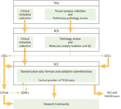
Figure 2. TCGA structure and relation between partners. TSSs (Tissue Source Sites) is responsible for

clinical metadata and biospecimen assemble from authorised cancer patients. BCR (Biospecimen Core Resource) then approves these data collected from TSSs. After approbal, processing and validation of the quality and quantity of sample, BCR registers and submits metadata to DCCs (Data Coordinated Centers). At the same time, molecular analysis are provided to GCCs (Genome Characterization Centers) and GSCs (Genome Sequencing Centers) for additional genomic characterization and high-throughput sequencing. Sequence-related data is stored in DCC. GSCs submits trace files, sequences, and alignment mappings to CGHub (NCI’s Cancer Genomics Hub secure repository). Then genomic data submitted to DCC and CGHub are made accessible to the research community and to GDACs (Genome Data Analysis Centers). GDACs supply new information-processing analysis and visualisation tools to the research community (Tomczak et al. 2015). ... 9

Figure 3. Representation of a SAM file. 1- Header Line. VN indicates the format version and SO the

sorting order alignment. 2- Sequence dictionary. SN represents de sequence name and LN the sequence length. 3- QNAME, Query template NAME. 4- FLAG, bitwise FLAG. 5- RNAME, Reference sequence NAME. 6- POS, 1-based left end mapping POSition. 7- MAPQ, MAPping Quality. 8- CIGAR, CIGAR string. 9- RNEXT, Reference name of the mate/NEXT read. 10- PNEXT, Position of the mate/NEXT read. 11- TLEN, observed Template LENgth. 12- SEQ, segment SEQuence. 13- QUAL, ASCII of phred-scaled base QUALity+33 (Li et al. 2009). ... 11

Figure 4. RNAseq samples distribution through tissue type and infection results in samples from CESC

cancer. ... 23

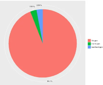
Figure 5. Percentage distribution of viral infection in CESC samples. Each sample was represented by

the virus with the higher ppm and only tumour tissue samples were considered in this graphic. Virus with ppm lower than 10 were not considered as infecting a sample. ... 24

Figure 6. Viral presence distribution in CESC cancer samples by ppm. Each column represents one

sample. Viruses with ppm smaller than 2 were not considered. ... 25

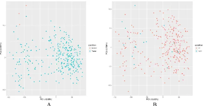
Figure 7. PCA of CESC samples. (A) Comparing samples between tumour and normal tissues. (B)

Comparing infected and not infected TP samples... 26

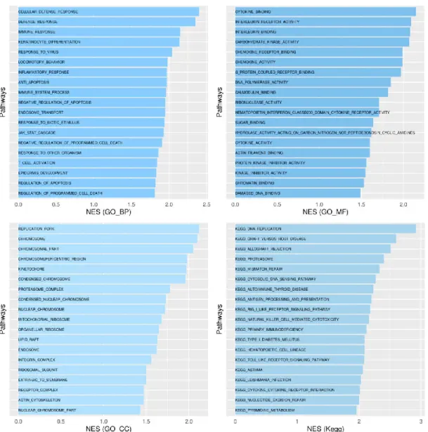
Figure 8. GSEA results for CESC when comparing infected and non-infected samples and using the

Gene Ontology Biological Process (GO_BP), Molecular Function (GO_MF) and Cellular Component (GO_CC), and the KEGG references lists. For each graphic 19 metabolic pathways with FDR smaller than 0.25 were picked and then sorted by NES value. The positive NES values mean that these are more expressed in the infected than in the non-infected. ... 28

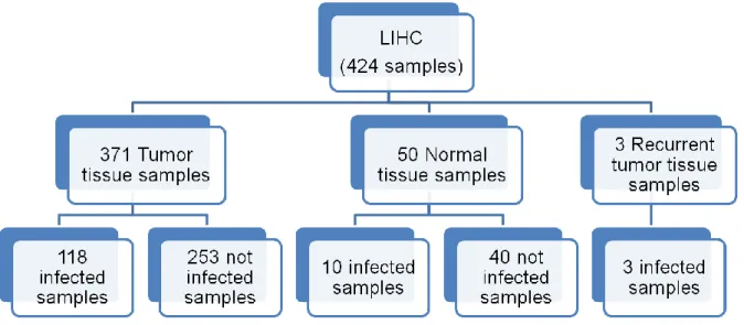
Figure 9. RNAseq samples distribution through tissue type and infection results in samples from LIHC

cancer. ... 30

Figure 10. Percentage distribution of viral infection in LIHC samples. Each sample was represented by

the virus with the higher ppm and only tumour tissue samples were considered in this graphic. Virus with ppm lower than 10 were not considered as infecting a sample. ... 31

Figure 11. Viral presence distribution in LIHC cancer samples by ppm. Each column represents one

xi

Figure 12. PCA of LIHC samples. (A) Comparing Samples from tumor and normal tissue. (B)

Comparing Samples from infected and not infected samples from TP samples only. ... 33

Figure 13. GSEA results for LIHC when comparing infected and non-infected samples and using the

Gene Ontology Biological Process (GO_BP), Molecular Function (GO_MF) and Cellular Component (GO_CC), and the KEGG references lists. For each graphic 26 metabolic pathways with FDR smaller than 0.25 were picked and then sorted by NES value. The positive NES values mean that these are more expressed in the infected than in the non-infected. ... 34

Figure 14. LIHC Somatic Mutations. (A) Global count of somatic mutations in 193 LIHC samples. (B)

Each somatic mutation type ratio (number of mutations found and divided by the number of sample) per infected and non-infected samples. ... 35

Figure 15. Pathways having a significant amount of genes hit by somatic mutations in infected and

non-infected LIHC groups obtained through G:Cocoa when running against Gene Ontology Biological Process (BP), Molecular Function (MF) and Cellular Component (CC), and the KEGG references lists. ... 36

Figure 16. RNAseq samples distribution through tissue type and infection results in samples from

HNSC cancer. ... 37

Figure 17. Percentage distribution of viral infection in HNSC samples. Each sample was represented

by the virus with the higher ppm and only tumour tissue samples were considered in this graphic. Virus with ppm lower than 10 were not considered as infecting a sample. ... 37

Figure 18. Viral presence distribution in HNSC cancer samples by ppm. Each column represents one

sample. Viruses with ppm smaller than 2 were not considered. ... 39

Figure 19. PCA of HNSC samples. (A) Comparing Samples from tumor and normal tissue. (B)

Comparing Samples from infected and not infected samples from TP samples only. ... 40

Figure 20. GSEA results for HNSC when comparing g infected and non-infected samples and using

the Gene Ontology Biological Process (GO_BP), Molecular Function (GO_MF) and Cellular Component (GO_CC), and the KEGG references lists. For each graphic 29 metabolic pathways with FDR smaller than 0.25 were picked and then sorted by NES value. The positive NES values mean that these are more expressed in the infected than in the non-infected. ... 41

Figure 21. HNSC Somatic Mutations. (A) Global count of somatic mutations in 279 HNSC samples.

(B) Each somatic mutation Ratio (number of mutations found and divide them by the number of sample) per infected and non-infected samples. ... 42

Figure 22. Pathways affected by somatic mutations in infected and non-infected HNSC samples

obtained through G:Cocoa when running against Gene Ontology Biological Process (BP), Molecular Function (MF) and Cellular Component (CC), and the KEGG references lists. ... 43

Figure 23. Comparison between CESC and HNSC cancer expression profiles. Only infected samples

from each cancer were used and were identified by the presence or absence of any HPV virus. ... 45

Figure 24. Distribution of HPV16 expressed genes when infecting CESC and HNSC samples. ... 46 Figure 25. Distribution of HBV expressed genes when infecting LIHC samples. ... 47

xii

T

I

Table 1. List of sets of information from each group of access (Zhang et al. 2011). ... 8 Table 2. Count of samples bearing infection in each cluster of the PCA of Figure 7B. The percentage

was calculated using the number of samples infected by each virus with ppm>10 and the total of infected samples in each cluster (61 samples in the left cluster and 225 in the right cluster). ... 27

Table 3. VirusSeq results of HNSC sample TCGA-BA-4077-01B. Confirmation of HPV16 insertion

on an infected sample and its correspondent expressed genes and location on the host genome. ... 44

xiii

L

A

BAM – Binary Alignment/Map format BC – Bonferroni correction

BCR – Biospecimen Core Resource CDS – coding sequences

CESC – Cervical carcinoma

CGHub – NCI’s Cancer Genomics Hub

se-cure repository

DCC – Data Coordinated Centers DNAseq – DNA sequencing EBV – Epstein Barr virus ES – Enrichment Score FDR – False Discovery Rate

GCC – Genome Characterization Centers GDAC – Genome Data Analysis Centers GO – Gene Ontology

GO_BP – Gene Ontology Biological

Pro-cess

GO_CC – Gene Ontology Cellular

Compo-nent

GO_MF – Gene Ontology Molecular

Function

GSC – Genome Sequencing Centers GSEA – Gene Set Enrichment Analysis HAdV – Adeno-associated virus

HBV – hepatitis B virus HCV – hepatitis C virus HHV – herpesvirus

HIV – The human immunodeficiency virus HNSC – Head and neck squamous cell

car-cinoma

HPV – Human papillomavirus HTS – high-throughput sequencing

ICGC – The International Cancer Genome

Consortium

LDL-R – low-density lipoprotein receptor LD – lipids droplets

LIHC – Hepatocellular carcinoma MCV – molluscum contagiosum virus miRNAseq – MicroRNA sequencing NAFLD – non-alcoholic fatty liver disease NCI – the National Cancer Institute NES – Normalized Enrichment Score NGS – next generation sequencing

NHGRI – National Human Genome

Re-search Institute

NIH – US National Institutes of Health NT – normal tissue samples

PC – principal components

PCA – principal component analysis PLAT – Percutaneous local ablative

ther-apy

ppm – parts per million RFA – radiofrequency ablation RNAseq – RNA sequencing

RPPA – Reverse-phase protein array SAM – Sequence Alignment/Map format TCGA – The Cancer Genome Atlas TP – tumour tissue samples

1

1. I

In the past, the occurrence of “house cancers” started the idea that cancer could be caused via some infectious agents. These “house cancers” were known to occur in people living in the same place, mostly between married couples and transmitted from mother to child. In the 19th century, these observations encouraged studies that could test the idea of development of can-cer malignancies through bacteria, fungi or parasites. Initially, these studies were unsuccessful in finding such agents, leading to a step-back in the hypothesis for many years (McLaughlin-Drubin and Munger 2008).

Some significant researches revealed cancer formation with cell-free transmission in non-malignant tumours in animals, but not in human models (McLaughlin-Drubin and Munger 2008). This was the case of Francis Peyton Rous experiments in 1911 that showed that the sarcomatous chest tumour on chicken could be transmitted over cell-free tumour excerpts, con-firming once more the hypothesis of the involvement of small infectious agents. Like many before him, these studies were treated like curiosities for many years. Only in the 1950s, after Ludwik Gross proved that murine retrovirus and polyomavirus induced murine cancers, Rous research was fully appreciated and awarded a Nobel Prize in 1966 (McLaughlin-Drubin and Munger 2008; Moore and Chang 2010).

Following the success in proving viral infection in animal cancers, a crescent number of scientists started a demand to discover oncogenic viruses in humans. Yet, it would take more 53 years since Rous’s famous research for the first human oncogenic virus to be observed. In 1964, during a study in cell lines of Burkitt’s lymphoma from African pediatric patients, An-thony Epstein, Bert Achong and Yvonne Barr identified small particles on the electron micro-scope. These particles were then identified as a virus by virological studies and named Epstein Barr virus (EBV) in their honour (Morales-Sánchez and Fuentes-Pananá 2014; Moore and Chang 2010). Later on, in 1970, hepatitis B virus (HBV) was discovered by D. S. Dane in human cells by using hepatitis B surface antigen (McLaughlin-Drubin and Munger 2008). Thanks to these two studies and to the development of model systems, additional studies on viral infection in cancer led to the identification of seven more oncogenic viruses, suggesting that more viruses important in cancer development can still be discovered (McLaughlin-Drubin and Munger 2008; Morales-Sánchez and Fuentes-Pananá 2014).

2

1.1. Viral Infection in cancer

Surprisingly, only a small portion of people infected with oncogenic viruses actually de-velop cancer, and an even smaller part of that group of people transmits the infection. Cancers seem to be a final event of the viral infection, and eventually lead to host death and viruses destruction (Moore and Chang 2010; Morales-Sánchez and Fuentes-Pananá 2014). Tumour viruses usually maintain their persistence in the host by creating a chronic infection during a period of many years, with a very small production, or almost none, of viral particles (Morales-Sánchez and Fuentes-Pananá 2014).

Studies through the past century led to the conclusion that infectious agents (viruses, bacte-ria and parasites) should be divided in two groups in relation to their involvement in cancer: direct and indirect carcinogens.

Direct carcinogen agents can be found in the cancer cells in a monoclonal form, which in-dicates that these agents are responsible for tumour cell transformations by keeping the carcin-ogen phenotype through expressing at least one transcript. This onccarcin-ogenic persistence is main-tained by viral formation of episomes or incorporation into the host genome (Morales-Sánchez and Fuentes-Pananá 2014; Moore and Chang 2010). In summary, direct carcinogen viruses have three essential characteristics: the viral genome can be found in every tumour cell; once host cells have grown, the virus can immortalize; and the virus causes cell transformation, im-mortalization and migration by disturbing the cell normal functioning (Chen et al. 2014). Hu-man papillomavirus (HPV), EBV and molluscum contagiosum (MCV) are examples where this activity is easily seen (Figure 1A) (Morales-Sánchez and Fuentes-Pananá 2014; Moore and Chang 2010; Chen et al. 2014).

On the other hand, indirect carcinogen agents lead to cancer through infection and inflam-mation that eventually causes cell mutation, showing that these agents are not restricted to remain inside the host cells (Morales-Sánchez and Fuentes-Pananá 2014; Moore and Chang 2010). Thus, these viruses work over two principal ways: starting chronic inflammation and immunosuppression. Chronic inflammation is initiated by chemokines produced by mutated cells that attack immune cells and injure local tissue. In this way, this kind of tumour activity resumes to a cycle between infections, inflammations and local tissue destruction (Figure 1B). In a similar manner, the immunosuppression process stars with an immune response failure.

3

The most common example of this process is displayed by HIV virus, which infection is re-sponsible for lowering the host defences and consequently increasing the risk of new infections to occur in the host (Figure 1C) (Morales-Sánchez and Fuentes-Pananá 2014).

A.

B.

C.

Figure 1. Direct and indirect viral carcinogenesis processes (images taken from Morales-Sánchez et al. 2014). (A) Represen-tation of direct viral carcinogenesis. Superior Section: Formation of episomes by viral genomes (e.g. herpesvirus). Lower Section: Viral integration into de host DNA (e.g. retroviruses). (B) Representation of chronic inflammation of indirect viral carcinogenesis. Production of chemokines from infected cells which attack immune cells and damage the local tissue. (C) Representation of immunosuppression of indirect viral carcinogenesis. Immunosuppression is caused by HIV and EBV infec-tion, and is controlled by cytotoxic CD8 T cells. While HIV infection develops, immune system starts failing and the host becomes more venerable to EBV infection (Morales-Sánchez and Fuentes-Pananá 2014).

Still, there are many viruses that cannot be classified only into direct and indirect mecha-nisms, such as HBV and HCV (hepatitis C virus). HBV genome is integrated into the host cells in almost all HBV-related tumours, however it is still not clear if the virus requires cell prolif-eration to maintain the genome transcription or not. Nevertheless, this type of classification is

4

still important, as it is a practical way to classify cancers that have a bigger chance of occurring via the action of oncogene viruses (Morales-Sánchez and Fuentes-Pananá 2014; Moore and Chang 2010).

Some studies have recently showed new techniques for viral detection on high-throughput DNA and RNA sequencing. These new studies allow an efficient unbiased detection of viruses in extended collections of data from cancer samples, overcoming limitations of studies based on low-throughput methodologies. One such study was performed by Tang et al. (2013), whom mapped virus infection in 4,433 samples from 19 human cancers, by using human centred RNASeq data. The inference based on RNASeq guarantees that the viral genome is being tran-scribed and that the infection is active. From the results obtained by Tang study it is possible to acknowledge that cervical (CESC), hepatocellular (LIHC) and head and neck squamous cell (HNSC) carcinomas are the top three cancers with higher viral infection rates (96.6%, 32.4% and 14.8%, respectively) (Tang et al. 2013). However, this work was based in a limited number of the samples now available in TCGA: 87 of 309 for CESC (28%); 34 of 424 for LIHC (8%); and 304 of 566 for HNSC (54%).

1.1.1. Cervical carcinoma (CESC)

Nowadays, the second principal cause of female death is cervical cancer. Thanks to large endorsements for vaccination and constant control through Papanicolaou test (Pap test), the frequency of this carcinoma dropped drastically in developed countries, but not yet in devel-oping countries, where 80% of cases occur (Adams et al. 2014; Muñoz et al. 2003). HPV has been reported in closely 100% of cervical cancers, mainly the high risk HPV16 and HPV18 strains. This infection can occur from sexual contact or via vertical transmission from mother to child during pregnancy or during birth (Adams et al. 2014).

Even if many women are infected with HPV, in most cases the immune cells eliminate the infection agents, and only a small portion of infected woman will progress from infection to cervical cancer. These women normally manifest immunity deficiencies caused by inherent genomic instability or because of bad life style habits, like smoking (Adams et al. 2014; Canavan and Doshi 2000).

1.1.2. Hepatocellular carcinoma (LIHC)

Hepatocellular carcinoma is one of the most common cancers worldwide and one of the most rapid cause of death. This cancer is common in Asia and Africa, but recently it is also

5

rising in America and Europe (Siegel and Zhu 2009; Chen et al. 2006). The principal risk fac-tors for LIHC are known to be abusive alcohol consumption and infection through HBV and HCV; however, it has been reported that 5-30% of the patients are cryptogenic (unknown dis-ease cause). The majority of LIHC cases are associated to a metabolic syndrome manifested in the liver named non-alcoholic fatty liver disease (NAFLD), consisting in fat deposits in liver cells in absence of any history of excess alcohol consumption. NAFLD is also related with insulin resistance, obesity, diabetes, dyslipidemia, and other metabolic conditions (Siegel and Zhu 2009).

The best treatment to this cancer is still the partial hepatectomy, though it is only applicable to about 9-27% patients. Percutaneous local ablative therapy (PLAT) and radiofrequency ab-lation (RFA) are being applied and allowing a better cancer control (Chen et al. 2006).

1.1.3. Head and neck squamous cell carcinoma (HNSC)

This cancer occurs 90% of the times from squamous cell carcinomas in mucosal surfaces in the neck and head. The principal risk factors have been reported to be dangerous life style habits, like ultraviolet light exposure and tobacco and alcohol consumption. Recently it was proved that HPV infection is a major cause, mostly in oropharyngeal cancer (tonsillar and base of tongue cancer). Till recently, 66% to 95% of the cases occurred in men after 50 years of age, but with the increasing number of female smokers this number tends to vary (Adams et al. 2014; Egloff et al. 2014).

Patients diagnosed with this cancer and HPV positive showed improvement and higher sur-vival rates when treated with chemotherapy, radiation and surgery, than the HPV negative counterparts. This led to the idea that HPV condition is a good biomarker of HNSC. As no diagnostic tools are available, HNSC patients must check for persistent symptoms such as ach-ing throats, inflamed glands and oral wounds (Adams et al. 2014).

1.2. Lipids influence in viral carcinogenesis infection

Lipids are the most important components in cell membranes, playing important roles in many biological functions like cell growth and division, energy production, motioning, mainte-nance of cell membrane integrity, activity of membrane enzymes, and DNA helix stabilization (Raju et al. 2014). Cholesterol is a lipid that executes some of those functions, and the lipopro-tein receptors placed in the cell surface are responsible for its absorption and control within cells. This mechanism is very important during membrane fusion for entry of virions in the

6

cells and during particle maturation. Taking the example of non-enveloped viruses, its capsid interacts with the host membrane and usually controls some of the membrane constituents, like glycosphingolipids, to start the viral infection. Some viruses, like HCV, can even induce viral entrance with functional low-density lipoprotein receptor (LDL-R) (Heaton and Randall 2011). Likewise, lipids play an important role during the viral life cycle since this occurs in the membranous cell organelles (as endoplasmic reticulum), assisting the membrane curvature and drafting core proteins to enable the construction of virus particles (Heaton and Randall 2011; Konan and Sanchez-Felipe 2014). Other example of its importance is the recognition of lipids droplets (LDs) as sites for assembly of some viruses (e.g. HCV). LDs are organelles derived from endoplasmic reticulum which are abundant in cholesterol esters and triglycerides (Konan and Sanchez-Felipe 2014). Furthermore, there are some changes in lipid metabolism and in specific lipid species, which are expected to be important in viral replication, assembly and secretion events. Some of those changes are the increase of flux metabolic directed into fatty acid biosynthesis pathway (visible in metabolic analysis of cytomegalovirus infection), and the inhibition of cholesterol and sphingolipids biosynthesis, or knockdown of proteins involved in their transport (visible during HCV production) (Heaton and Randall 2011; Konan and Sanchez-Felipe 2014).

In the other hand, oncogenic studies have showed that cholesterol is found in low concen-tration and can indicate a continuous oncogenic process, in some growing tissues and blood partitions (Singh et al. 2013). So far, most claims of variations in lipid profiles among normal and tumour cells (like in CESC and HNSC) (Raju et al. 2014; Singh et al. 2013) have been associated with bad life habits like the use of tobacco, and not with infection. It has been re-ported that tobacco carcinogens are responsible for greater amount of peroxidation of polysatu-raded fatty acids through induction of free radicals and production of reactive oxygen species. This lipid peroxidation can heavily disturb fundamental membrane cell components and may lead to carcinogenesis since, because of it, great utilization of lipids like cholesterol, lipopro-teins and triglycerides is needed for membrane syntheses of the new cells. In order to provide for these needs, lipids are taken from blood circulation, degraded from lipoproteins or metab-olised.

The elucidation of the involvement of lipids in cancer is very important, namely in terms of treatment. Some studies have shown that antioxidant vitamins have a great defensive influence against lipid peroxidation (Patel et al. 2004). It was also suggested that cancer cells or several minor malfunctions during the lipid or antioxidant vitamin metabolism can be responsible for

7

the drop of lipid concentration that occurs during hypolipidemia (Raju et al. 2014; Singh et al. 2013; Patel et al. 2004). Yet, these associations are controversial since many studies have re-ported a different relation between cancer and lipid profile parameters (Raju et al. 2014; Patel et al. 2004). It is also not yet guaranteed that cancer diagnosis through lipid parameters is viable (Raju et al. 2014).

1.3. Database and bioinformatic tools

Following the publication of the human genome sequence, an increase in larscale ge-nome studies has taken place, namely in the cancer research field. Soon after, the idea of a unified record of cancer genomes emerged in order to deal with the following issues: independ-ent tumour genome studies could lead to investmindepend-ent of resources in the same type of cancer instead of broadening the spectre of types of cancer studied; the absence of normalisation be-tween the different studies could produce noise and biases in the analyses and comparisons; the existence of many cancers that differ through the world should lead to a coordinated strat-egy between local consortia; and the fact that only one organisation could coordinate and, con-sequently, accelerate the distribution of data and a more efficient analysis (Hudson et al. 2010).

Researchers and funding agency councils from 22 countries, encouraged from that initial idea, gathered in late 2007 in Toronto, Canada, to decide the best way to proceed. The Interna-tional Cancer Genome Consortium (ICGC) was launched, aiming to perform a comprehensive and high-throughput analysis of tumours in an organized way (Zhang et al. 2011). Given the dimension of this challenge, operational groups were formed in order to create policies and plans that would form the base requirements to participate in the ICGC (Hudson et al. 2010).

In order to hasten cancer research, the consortium has as main goals: (1) the creation of complete sets of genomic anomalies in tumours of 50 distinct cancer types and subtypes, in high resolution, fullness, high quality and controlled data; (2) form complementary lists of transcriptomic and epigenomic datasets from the correspondent tumours; and (3) allow the whole investigation community to have access to the data obtained promptly with the least limitations. Thus, ICGC also organized the research community so that no repeated researches occur, and promoted the proliferation of new technologies, software and techniques (Hudson et al. 2010; Zhang et al. 2011).

8

The large amount of genetic information available in these databases raises bioethical issues, particularly concerning the patient anonymity. Since the genomic data allow individual identi-fication, data access policies were developed in order to protect that information. Those access policies consist in dividing the dataset into two different sets (Table 1). The first set will contain accessible information and will not have data capable of identifying the individual identity. The second set will be the most restricted group, and although it will not contain direct identi-fication of the individual, it will have complex genomic and clinical data that belong to a unique human being. The permission of access to the second set can only be given by the Data Access Compliance Office to researchers that submit their project (Hudson et al. 2010; Zhang et al. 2011).

Table 1. List of sets of information from each group of access (Zhang et al. 2011).

ICGC Open Access Datasets ICGC Controlled Access Datasets

 Cancer Pathology

 Histologic type or subtype  Histologic nuclear grade  Patient/Person

 Gender  Age range

 Gene Expression (normalized)  DNA methylation

 Genotype frequencies

 Computed Copy Number and Loss of Heterozygosity

 Newly discovered somatic variants

 Detailed Phenotype and Outcome Data  Patient demography  Risk factors  Examination  Surgery  Drugs  Radiation  Sample  Slide

 Specific histological features  Protocol

 Analyte  Aliquot

 Gene Expression (probe-level data)  Raw genotype calls

 Gene-sample identifier links  Genome sequence files

Initially, the consortium started by including two European consortia and 10 participating countries, but currently the number increased to 15 (Hudson et al. 2010). Another important project that contributed to ICGC development was The Cancer Genome Atlas (TCGA). This project is older than ICGC, and it was initiated by the US National Institutes of Health (NIH). These two related projects were the main factors of the great growth of complete comprehen-sion of cancer genomes (Hudson et al. 2010).

9 1.3.1. TCGA

The Cancer Genome Atlas is a public funded project by the US National Institutes of Health and was created as a Pilot Project from the Nacional Institute of Health (NIH) in 2006, with similar aims to ICGC but at a local scale in the US. It is currently using large-scale genome sequencing and multi-dimensional analyses in order to characterise above 30 human cancers (Hudson et al. 2010; Tomczak et al. 2015).

Figure 2. TCGA structure and relation between partners. TSSs (Tissue Source Sites) is responsible for clinical metadata and biospecimen assemble from authorised cancer patients. BCR (Biospecimen Core Resource) then approves these data collected from TSSs. After approbal, processing and validation of the quality and quantity of sample, BCR registers and submits metadata to DCCs (Data Coordinated Centers). At the same time, molecular analysis are provided to GCCs (Genome Charac-terization Centers) and GSCs (Genome Sequencing Centers) for additional genomic characCharac-terization and high-throughput se-quencing. Sequence-related data is stored in DCC. GSCs submits trace files, sequences, and alignment mappings to CGHub (NCI’s Cancer Genomics Hub secure repository). Then genomic data submitted to DCC and CGHub are made accessible to the research community and to GDACs (Genome Data Analysis Centers). GDACs supply new information-processing analysis and visualisation tools to the research community (Tomczak et al. 2015).

TCGA is well structured and divided in many partners who are responsible for different tasks, from the sample gathering and manipulation, to high performance methods based on microarrays and next-generation sequencing, and respective bioinformatic data analysis (Tis-sue Source Sites, Genome Characterization Centers, Genome Data Analysis Centers, etc.). For a better understanding of the cancer omics, different approaches have been applied: RNA se-quencing (RNAseq), MicroRNA sese-quencing (miRNAseq), DNA sese-quencing (DNAseq), SNP-based platforms, Array-SNP-based DNA methylation sequencing, and Reverse-phase protein array (RPPA) (Tomczak et al. 2015).

10

NIH, the National Cancer Institute (NCI) and the National Human Genome Research Insti-tute (NHGRI) established partnerships with other North American and European instiInsti-tutes, and in 2010 TCGA data was largely incorporated the ICGC Data Portal (Tomczak et al. 2015). Yet, TCGA is not allowed to officially become ICGC’s member for legal and technical manners, once it belongs to the US’s NIH (Figure 2) (Hudson et al. 2010).

1.3.2. Bioinformatic tools

With the growing number of available genomic data, the demand on fast and efficient anal-yses led to the need of developing new bioinformatics tools. Many of the recently implemented tools were used by Tang et al in 2013 that, in fact, proved their applicability. Some of the studies performed in this thesis are based on the pipeline implemented by Tang and his col-leagues.

1.3.2.1. SAMtools

The first step on the processing of data is the alignment for a competent read mapping against a reference sequence. Diverse alignment tools were available but generated different formats that made complex the downstream processing, and rendering it urgent to develop an universal format. This led to the genesis of the Sequence Alignment/Map (SAM) format (Fig-ure 3) (Li et al. 2009).

The SAM format is simple and flexible, once it can retain information from numerous se-quencing platforms and read aligners, and supports single and paired-ended reads and blending reads of various types. This format is prepared to support alignment sets over 1011 base pairs which is approximately the size needed for a human genome. A similar format is the Binary Alignment/Map (BAM) format, which consists in a binary representation of the SAM format. Basically it has the same information of a SAM file but is represented in a more compacted way that can process information from a particular location in the genome without loading the entire file data, in order to improve performance (Li et al. 2009). Nowadays, almost all genomic studies use SAM/BAM files as the base files for diverse types of analyses. But many of the current informatic methods take too much RAM memory and require several CPUs, so it is very important to use the correct and more appropriate tools for each research (Langmead et al. 2009).

11

Figure 3. Representation of a SAM file. 1- Header Line. VN indicates the format version and SO the sorting order alignment.

2- Sequence dictionary. SN represents de sequence name and LN the sequence length. 3- QNAME, Query template NAME. 4- FLAG, bitwise FLAG. 5- RNAME, Reference sequence NAME. 6- POS, 1-based left end mapping POSition. 7- MAPQ, MAPping Quality. 8- CIGAR, CIGAR string. 9- RNEXT, Reference name of the mate/NEXT read. 10- PNEXT, Position of the mate/NEXT read. 11- TLEN, observed Template LENgth. 12- SEQ, segment SEQuence. 13- QUAL, ASCII of phred-scaled base QUALity+33 (Li et al. 2009).

SAMtools consists in a collection of software packages which par and manipulate the exist-ent alignmexist-ents in the SAM/BAM files and have the capability to: (1) sort and combine align-ments; (2) exchange other alignment formats to SAM or BAM format; (3) eliminate PCR rep-licas; (4) call SNPs and short indel variants; (5) create an output with information listed per-position; and (6) show this output in a text-based format (FASTA) (Li et al. 2009).

The only disadvantage of this software is the fact that it takes a little too long for alignment and indexing of data. For example, to use a MAQ file with 112GB it takes about 10h to convert it and 40 min to index it with less than 30 MB of memory. This tool has implementations using two different languages, Java and C, which grant different functionalities. Since SAMtools is such an efficient tool, for the past six years it has become a crucial instrument for next gener-ation sequencing (NGS) alignment studies (Li et al. 2009).

1.3.2.2. PRINSEQ

PRINSEQ is a bioinformatic tool that is used to filter, reformat and trim NGS data, and that is used to create a pre-processing statistic synopsis of data and of its quality, permitting an efficient control before any downstream study being made (Schmieder and Edwards 2011). This tool supports FASTA, FASTQ and QUAL files of genomic and metagenomic datasets, and it was implemented in two different ways: (1) in a web interface, which is very easy to use; and (2) a standalone lite version (Schmieder and Edwards 2011). The principal difference be-tween these two versions is that the standalone version does not create any statistic synopsis in graphical form.

12 1.3.2.3. Bowtie

Bowtie was developed to create an ultrafast, memory-efficient short read aligner optimized for mammalian re-sequencing. Bowtie can align short DNA sequence reads to long sequences in a fast way and using an acceptable amount of RAM memory. By being based in full-text minute-space index, it applies Burrows-Wheeler indexing which results in a memory occupa-tion of 1.3GB for a human genome. With this low RAM memory occupaoccupa-tion, it allows an ordinary computer, with 2GB RAM, to use this software.

Bowtie was especially optimized to achieve the highest performance. Because of that if more than a match exists for the same read, it is assured that one will be reported, but not necessarily the best alignment. In other words, Bowtie may fail valid alignments if there are many mismatched reads. To avoid this, Bowtie has an option that increases the precision but it will reduce its performance (Langmead et al. 2009). This tool is very practical, and supports FASTA and FASTQ files, and Bowtie2 supports also insertions, deletions or paired-end align-ments (Langmead et al. 2009; Langmead and Salzberg 2012).

1.3.2.4. Picard Tools

Set of bioinformatics tools for high-throughput sequencing data manipulation compatible with SAM, BAM, CRAM and VCF files. All Picard Tools only work through command line and are provided as a single executable jar file (Java file) (Broad Institute 2016).

Even though there are around 80 tools available for a high variety of tasks, in this thesis we only used two of those tools – SamToFastq and MarkDuplicates. SamToFastq has as primary objective to convert SAM or BAM files into FASTQ. Furthermore, it also has options which allow to extract read sequences and base quality scores from the input files. In this thesis this tool will be mostly used to split whole genome files into forward and reverse sequences that will serve as input files in the bioinformatic tool VirusSeq (which will be explained below) in order to detect viral integration in human genomes (Broad Institute 2016).

MarkDuplicates locates and tags duplicated reads in BAM and SAM files. Then, these du-plicate reads are defined as originated from the same DNA fragment and acknowledged as read pairs which have identical 5’ positions for both reads in mate pair. As an output, a new SAM or BAM file is created with all duplicated sequences removed, identified in the SAM flag field, or even marked with a duplicate type in the “DT” optional attribute. Additionally, it also out-puts a second file with the number of read pairs examined, unmapped reads, unpaired reads, duplicated unpaired reads, duplicated read pairs and optical duplicated read pairs (duplicates

13

that appear clustered together during sequencing and can emerge from optical/image-pro-cessing artifacts or from bio-chemical processes during clonal amplification and sequencing) (Broad Institute 2016).

1.3.2.5. VirusSeq (with Mosaik)

As it was said before in this report, many viruses are related to human tumours and with the improvement of bioinformatic technologies it became possible to detect viral presence/infec-tion in human cells through the analyses of paired-end reads by VirusSeq. This algorithm uses NGS data and detects known viruses and its integration sites in the human genome.

This tool uses FASTQ format files with paired-end reads as input, and those reads can be whole-transcriptomic or whole-genomic data. The first step is the alignment to the reference genome, by using the program Mosaik (provided when VirusSeq is downloaded). This program is an aligner tool that, contrary to what happens with Bowtie, can compare at the same time the viral genome against the tumour genome in study so that the viral integration can be deter-mined. VirusSeq starts the identification of human and non-human sequences by aligning the input file with the human genome reference. Then, the non-human sequences are compared against the viral database in order to find any virus present in those sequences. The genome sequences of well-known viruses are all put together into one single chromosome named chrVirus, which will serve as a viral database. This viral database was combined with the hu-man reference genome hg19 making this reference genome named hg19Vrus where the chrVirus was designed as chr25 (Chen et al. 2013). With this strategy ViruSeq can, then, iden-tify if any of the viruses is infecting the inputted sample and describe its precise location when inserted in the human genome.

VirusSeq is a very effective tool, yet, it also has some crucial limitations: (1) the virus data-base must be updated frequently by the user (Chen et al. 2013); (2) it takes too much memory RAM, and an ordinary computer cannot run it; (3) and it takes a long time to run.

1.3.2.6. PCA

The big datasets being produced and analysed currently have a high amount of variables and variance contributing to it. This is the case of the expression profiles for the around 20,000 human genes that is inferred from RNAseq data. Several parameters can contribute with vari-ability to the human gene profile, besides the cancer and infection status, such as the date when the lab analysis was perform, the lab that performed it, the geographical origin of the sample,

14

etc. Some theoretical techniques allow to investigate the partitioned effect of the multifactorial variables, as the older and commonly used principal component analysis (PCA) (Jolliffe and Cadima 2016). PCA is a classical method which reduces de data dimension by transforming a new set of variables called principal components (PC) which are unrelated and orthogonal. PCs are ordered so that the kth PC have the kth higher variances of all PCs. As PCA can detect artefacts and biases, it is usually used as pre-processing phase (Y. Liang et al. 2005; Yao et al. 2012).

However, this technique is not perfect. It may fail when it comes to reproduce biology rela-tions. Recent studies have showed that microarray gene expression may have a super-Gaussian distribution, and the PCA method considers that gene expression follow a multivariate distri-bution. Also, PCA reduces the data based on the maximization of its variance, and sometimes biological problems do not relay on the data highest variance (Yao et al. 2012).

1.3.2.7. Gene Set Enrichment Analysis

Gene Set Enrichment Analysis (GSEA) is a computational process that evaluates differences among two biological states of a set of genes and determines if they are statistically significant (Subramanian et al. 2007). Its principal goal is to determine if a defined set of genes S are randomly distributed through a list L of mRNA expression profiles of genes ordered according to their differences. The GSEA method works on three principal steps: (1) calculation of an Enrichment Score (ES) that, shows the degree of representation of set S in the extremes of the entire ranked list L (top or bottom); (2) estimation of Significance Level of ES by using an empirical phenotype-based permutation test that conserves the correlation arrangement of the gene expression data; and (3) adjustment of estimated significance level to consider for multi-ple hypothesis testing (Subramanian et al. 2005). GSEA also offers the possibility to perform preranked analysis, where the gene set enrichment analysis is run against the ranked list of genes created during the default GSEA run. This allows to perform a correction of results from the default GSEA run, and to obtain more accurate values.

Two indicators are important in GSEA results, the False Discovery Rate (FDR) and the Normalized Enrichment Score (NES). FDR is the probability of a gene set represents a false positive; it is a ratio of the actual ES vs. the ES of all gene sets against all permutations of the dataset and the actual ES vs. ES of all gene sets against the actual dataset. On the other hand, the NES value represents, as its name indicates, the normalization of the ES value and can be used to compare analysis results all over the gene set.

15

There are many tools that execute similar functions as GSEA, but it is beyond doubt that GSEA continues to be the most used. Many have reported lack sensitivity of this method, how-ever many improvements have been made do correct that limitation. The fact that GSEA was conceived to find general dissimilarities in a cumulative distribution probably gave advantage of GSEA over other methods like z-test, which only could identify sets of genes with mean shifts (Irizarry et al. 2009).

1.3.2.8. G:Cocoa (G:Profiler)

It is known that most of the somatic mutations in cancer are usually unique events occurring independently in different patients, with the exception of the ones affecting oncogenes and proto-oncogenes (Lawrence et al. 2015). But these independent somatic mutations can affect the same metabolic pathways, and in our specific case, make infected individuals more suscep-tible to the viral infection. To test this we used G:Cocoa from G:Profiler webtool (Reimand et al. 2016).

G:Profiler is a public web server developed and maintained by the Institute of Computer Science of University of Tartu with the objective of characterising and manipulating gene lists of high-throughput genomics. This web server is currently available for over 80 species and has six available tools, as G:Cocoa tool used in this work (Reimand et al. 2016).

G:Cocoa is a enrichment tool which performs functional analysis of dozens of gene lists allowing a simple and minimal view of functional enrichments of those lists and providing a means to rank and compare gene lists through their functional annotations. Because of the mul-tiple functional enrichment analysis and its comparison against many reference lists, this tool performs a multiple testing correction which methodically reduces the significance of each p-value, discarding the number of false positive values. By default it is used the tailor-made al-gorithm g:SCS, otherwise the user may choose to use Bonferroni correction (BC) or Benaja-mini-Hochberg False Discovery Rate (Reimand et al. 2016).

1.3.2.9. HTSeq

HTSeq is a Python package which allows the fast processing and analysis of high-through-put sequencing (HTS) data. This tool receives as inhigh-through-put the most common file formats for ref-erence sequences, short reads, short read alignments, genomic feature, annotation and score data (FASTA, FASTQ, SAM/BAM, GFF, VCF, etc.). The principal component of this tool is

16

a container class which allows working with genomic coordinates (genomic positions or ge-nomic intervals) more simply. This tool contains two different applications: HTSeq-qa, for quality assessment; and HTSeq-count, for processing RNA-seq alignments for expression anal-ysis (Anders et al. 2015).

HTSeq-count receives as input SAM/BAM files from RNAseq data and GTF/GFF files with gene models. The number of times each gene had its exons overlapped in the aligned reads is counted. It is important to notice that ambiguous reads (reads which overlap with more than one gene or that align to various positions) are not considered. Even if this tool is written in Python, it can be run with simple shell commands without any Python knowledge. Also, this tool requires very little RAM memory, being able to process over 1.2 million reads per minute using around 250 to 450MB RAM, approximately (Anders et al. 2015).

17

2. A

In order to better understand the impact and effect of viral infection in cancer, this study has six principal aims:

1) to estimate infection rates in CESC, LIHC and HNSC from inference on the TCGA avail-able RNASeq data. The work of Tang et al. 2013 quantified in 425 samples belonging to these cancer types, but we enlarged to the full amount of 1299 samples currently available at TCGA. The lower quantity of cases checked in Tang et al. work will be used as quality control in our analysis;

2) to fully characterize the virus strains that are present in each infected individual, by using an updated human viral reference database, according to information deposited in NCBI;

3) to check if specific human pathways are associated with the infection, by performing gene enrichment analysis (using GSEA tool) between infected and non-infected groups in the three types of cancer;

4) to determine if infection is responsible for an increasing of somatic mutations, or if these are related with immune-related pathways;

5) to identify which viral genes are expressed during infection of the most prevalent viruses; 6) to detect viral insertion within a human genome.

18

3. M

3.1. Viral database

For the construction of the reference viral database, a list of accession numbers of all known human viruses was downloaded through the NCBI complete viral genome website. Then, all bacteriophages and endogenous viruses were removed from the list, making a final total of 5003 viruses. A Python script was created, to receive that list as input. Then, by using the Bio package provided freely by NCBI that contained the module Entrez and their efetch function, the genomes of all viruses in that list were downloaded into a single fastq file. This final fastq file was then used as reference database to investigate viral presence in the cancer samples.

3.2. Human raw RNAseq database

Since our intention was to investigate active viral infection, implying transcription of viral genes, we downloaded the dataset of raw RNAseq samples for each cancer. This dataset aimed to address the human transcriptome, but other non-human transcripts are also indirectly screened, namely viral transcripts.

The RNAseq data was downloaded from the CGHUB database, provided by TCGA, filter-ing the data only for RNAseq with HG19 assembly, accountfilter-ing to 309 samples from CESC cancer, 424 from LIHC and 566 samples from HNSC. All RNAseq samples were downloaded as BAM files and each sample had an average size of 7GB which corresponded to a total size of 8.62TB of downloaded information (2.14TB for CESC, 2.49TB for LIHC and 3.99TB for HNSC). In mean, around one week was needed for the download for each cancer type. Most of these RNAseq samples were from the solid tumor, but a few were from the solid normal tissue. We extracted both in order to do some comparisons.

3.3. Viral presence detection

Once all samples had been downloaded, the viral presence procedure could be implemented. Initially all BAM files were indexed through SAMTOOLS which allows to analyse directly specific parts of the BAM file without reading through all the sequence. In this case, SAMTOOLS allowed us to focus on the unmapped regions against the known human tran-scriptome, information previously processed by TCGA team. These unmapped regions were extracted from the BAM files and converted to fastq files. A quality control was then applied

19

to the fastq files, by using PRINTSEQ program, which removes reads with less than 45 nucle-otides.

Thereafter, Bowtie tool was used to align each sample (the cleaned fastq files of unmapped reads) against the viral database previously created, and limiting the data to 2 mismatches and a maximum of 25 valid alignments for each read, outputting the alignment in a SAM file for-mat.

Finally, we used SAMTOOLS and Picard Tools to remove duplicated reads from the SAM file and count how many times each virus was aligned within each sample. The final output is a text file with a list of viruses found in each sample and the number of times each virus aligned with that sample. This whole process took around 4 to 5 days to be completed for each cancer type analysed here in a dual-core computer with 4GB RAM memory.

3.4. Infection state determination in a cancer sample

Following others (Tang et al. 2013), we calculated the parts per million (ppm) value for each virus in each sample. In order to do that the number of each virus reads on that sample was divided by the total number of reads in the same sample and multiplied by one million, accord-ing to the followaccord-ing formula:

=

′ × 10

The total number of reads in the sample is the sum of all human and non-human reads which were previously determined using SAMTOOLS. We report all viruses present in a sample, even with low ppm, but we established a threshold for a sample to be considered as infected: when the most prevalent virus is >10 ppm.

3.5. Human transcriptomic profile and matrix construction

In order to investigate human gene expression differences between infected and non-in-fected groups, we used the gene expression values inferred by TCGA team and deposited in their database. Single files for each sample, with the complete list of normalized expression counts for all known human genes (20,531 genes), were downloaded (average of 400MB each) and merged into one matrix per cancer type. That matrix had in the first column the list of all genes and in the successive columns the normalized counts for each sample. A matrix with this

20

distribution was used in the GSEA software that we will discuss bellow, while a reverse one was used in the PCA analyses.

3.6. PCA

Gene expression is influenced by several factors that can lead to spurious or false results in statistical analyses of differential expression. In order to have an idea on the variance among the samples we performed principal component analyses (PCA) (Mardia et al. 1979) by using an R script. We controlled for variance between tumour and normal tissue samples, and be-tween infected and non-infected samples.

3.7. Gene Expression Analysis

For a gene expression enrichment evaluation between infected and non-infected groups, we performed a GSEA analysis (Subramanian et al. 2007). Both groups were constructed in order to have an equivalent number of individuals, controlled by the group with the lower number of samples and the other made of the same size by picking up samples at random controlling for the population group and geographical origin to which the individuals belonged. In the end, size of groups amounted to 18 in CESC, 118 in LIHC and 86 in HNSC.

This tool analyses if significantly differentially expressed genes are organised within known metabolic pathways, so it incorporates reference lists of metabolic pathways from diverse da-tasets as KEGG (Ogata et al. 1999) and Gene Ontology (Consortium 2001). We performed the analyses against KEGG and the three main Gene Ontology lists (Biological Process, Molecular Function and Cellular Component).

When running GSEA we used most of the default parameters, except for a small number of exceptions. First we started by changing the option “Collapse dataset to gene symbols” from True to False, since our matrix already had gene names there is no need to associate to any chip annotation file, and by setting the gene “Max size” and “Min size” parameters to 1000 and 5, respectively. This option allowed us to exclude from the analyses metabolic pathways having a too limited number of genes.

Once each GSEA run had finished we used the same data to do a Preranked run. We left almost all parameters as default only changing the “Collapse dataset to gene symbols”, the gene “Max size” and “Min size” parameters like we did previously on the normal GSEA run.