Licenciado em Ciências de Engenharia Mecânica
Numerical simulation of two-degree-of-freedom
vortex induced vibration in a circular cylinder
with OpenFOAM
Dissertação para a obtenção do Grau de Mestre em
Engenharia mecânica
Orientador: José Manuel Paixão Conde, Prof. Auxiliar, FCT - UNL
Júri
Presidente: Prof. Dr. José Fernando de Almeida Dias Vogais: Prof. Dr. Eric Lionel Didier
circular cylinder with OpenFOAM
Copyright © Pedro Daniel dos Santos Conceição, Faculty of Sciences and Technology, NOVA University of Lisbon.
First of all I would like to thank my supervisor, Prof. Dr. José Conde, for the guidance that he provided me along the development of this work.
I would like to express my gratitude to my family for all the comprehension and support.
To all of my friends for the companionship.
Computational fluid dynamics tools are capable to simulate the influence of a fluid flow passing around an object. The ability to predict the impact of such flows on a specific product performance is time consuming and costly without some form of simulation tool. In fact, across a wide range of engineering areas, virtual development allows the reduction of the number of prototypes and less testing until a product is ready to the market. Therefore, it is important to provide computational fluid dynamics users with easy-to-use, robust, time-efficient and validated processes. Bearing this in mind, the current thesis studies the phenomenon of vortex induced vibrations simulating a flow around an oscillatory cylinder.
A flow passing around a rhombic body originates dynamic forces which, consequently, induce a set of body movements that are well characterized in the literature. To perform the numerical investigation of this phenomenon was used the OpenFOAM, an open-source software which is numerically able to perform a detailed and accurate analysis of this complex phenomena. Given the few scientific studies about the vortex induced vibration phenomenon with two degrees of freedom, this thesis aims to validate the Open-FOAM software for this case study, providing the scientific community the validation of a new numerical tool for studies of this kind. With this goal, it was firstly performed a mesh independence study for a flow around a fixed cylinder where it was studied the influence of the mesh on the fundamental quantities, that is, the Strouhal number, St, the mean drag coefficient,CD,mean, and the root mean square of the drag,CD,rms, and lift,
CL,rms, coefficients.
Then, it was carried out the study of the flow around a cylinder with one degree of freedom. It was studied the response of the cylinder for two types of systems, mass-spring system and mass-spring-damper system for a mesh with a 2500Ddomain length. The obtained results where then compared with the data described in the literature for a 50D
length mesh, allowing to infer which is the impact of the mesh size into the obtained results.
comparative study showed an asymmetric movement of the cylinder. Given this data, it was hypothesised and proven that this fact was associated with the non-symmetry of the mesh used by the literature paper.
As ferramentas de dinâmica dos fluidos computacional têm a capacidade de simular qual a influência que um dado escoamento tem ao interagir com um corpo. De facto, sem uma ferramenta de simulação, predizer qual o impacto que determinado escoamento tem na performance de dado produto é moroso e dispendioso. Este facto faz com que, em diver-sas áreas da engenharia, a análise virtual permita a redução do número de protótipos e os testes necessários para colocar um produto no mercado. Assim, é importante fornecer aos utilizadores de ferramentas de simulação na área de dinâmica dos fluidos ferramentas fáceis de usar, robustas e com processos validados. Com este objetivo em mente, a pre-sente tese pretende estudar o fenómeno de vibrações induzidas por vórtices através da simulação de um escoamento em torno de um cilindro oscilatório.
Um escoamento ao passar por um corpo rômbico origina forças dinâmicas que provo-cam um conjunto de movimentos característicos deste fenómeno e que estão bem carac-terizados na literatura. Para proceder à análise numérica deste fenómeno foi utilizado o OpenFOAM, este é um softwarede uso livre que se entendeu ser numericamente capaz de realizar uma análise suficientemente detalhada e correta deste fenómeno complexo. Tendo em conta os escassos estudos científicos sobre o fenómeno da vibração induzida por vórtices para um corpo com dois graus de liberdade, esta tese tem como objetivo a validação dosoftwareOpenFOAM para este caso de estudo, disponibilizando à comuni-dade científica a validação de uma nova ferramenta numérica para realizar estudos deste género. Para tal ser possível, começou por se estudar a independência da malha para o escoamento em torno de um cilindro fixo analisando qual a influência que a malha tem nas quantidades fundamentais, ou seja, o número de Strouhal,St, a média do coeficiente de arrasto,CD,mean, e a raiz do valor quadrático médio dos coeficientes de arrasto,CD,rms, e de sustentação,CL,rms.
De seguida, foi efetuado o estudo do escoamento em torno de um cilindro com um grau de liberdade. Foi analisada a resposta dada pelo cilindro para dois tipos de sistemas, sistema massa-mola e sistema massa-mola-amortecedor para uma malha de domínio 2500D. Os resultados obtidos foram posteriormente comparados com dados descritos na literatura para uma malha de domínio 50D, possibilitando averiguar qual o impacto do tamanho da malha nos resultados obtidos.
foram comparados com os dados descritos na literatura para um estudo semelhante. A maior diferença entre os resultados de ambos os estudos foi a simetria do movimento oscilatório do cilindro que foi obtida para o presente estudo enquanto que o estudo comparativo apresentou um movimento assimétrico do cilindro. Com isto, foi proposto e demonstrado que este facto está associado com a não-simetria da malha utilizada pelo artigo da literatura.
List of Figures xv
List of Tables xix
Acronyms xxi
Nomenclature xxiii
1 Introduction 1
1.1 Context and motivation . . . 1
1.2 Problem formulation . . . 2
1.3 Original contributions . . . 3
1.4 Thesis layout . . . 3
2 Theoretical contextualization 5 2.1 Fundamentals of a flow around a circular cylinder . . . 5
2.1.1 Disturbed regions in a circular cylinder . . . 6
2.1.2 Transition in disturbed regions . . . 6
2.1.3 Types of the flow states . . . 7
2.1.3.1 Laminar state of flow,L . . . 7
2.1.3.1.1 "Creeping" flow,L1. . . 8
2.1.3.1.2 Steady separation regime,L2 . . . 10
2.1.3.1.3 Periodic laminar regime,L3. . . 11
2.1.3.2 Transition-in-wake state,TrW. . . 14
2.1.4 Vortex shedding and vortex patterns . . . 17
2.1.5 Response modes for a cylinder with one-degree-of-freedom in trans-verse motion, Y-only . . . 20
2.1.6 Response modes for a cylinder with two-degrees-of-freedom inXY -motion . . . 23
2.2 Fundamentals of Vibration . . . 27
2.2.1 Two-Degree-of-Freedom Systems . . . 29
2.3 Computational Fluid Dynamics: mathematical equations modelling the
fluid flow . . . 34
2.3.1 Finite Volume Method . . . 35
2.3.2 Conservation of Mass . . . 36
2.3.3 Conservation of Linear Momentum . . . 36
2.3.4 Conservation of Energy . . . 36
2.3.5 Newtonian Fluids . . . 37
2.3.6 The Navier-Stokes Equation . . . 37
3 Numerical modelling methodology 39 3.1 Mesh generation using Gmsh . . . 40
3.1.1 Important mesh parameters . . . 40
3.1.2 Mesh geometry . . . 42
3.1.3 State-of-the-art: mesh generation tools . . . 42
3.2 Computational fluid dynamics analysis using OpenFOAM . . . 43
3.2.1 Finite volume mesh . . . 45
3.2.2 The PIMPLE Algorithm . . . 46
3.2.3 Case study setup - OpenFOAM File System overview . . . 46
3.2.3.1 CaseStudy/0folder - initial conditions . . . 46
3.2.3.2 CaseStudy/constantfolder - initial conditions . . . 48
3.2.3.3 CaseStudy/systemfolder - system parameters . . . 48
3.2.4 State-of-the-art: computacional fluids dynamics tools . . . 48
3.3 Numerical Stability . . . 49
3.4 Simulations preformance . . . 50
4 Flow around a fixed cylinder 51 4.1 Independence mesh study . . . 51
4.1.1 Analysis of the fundamental quantities convergence with the2500D mesh discretisation . . . 51
4.1.2 Analysis of the fundamental quantities convergence with the time step for a mesh with2500Ddomain length . . . 56
4.1.3 Analysis of the fundamental quantities convergence with the do-main length . . . 57
4.1.4 Analysis of the fundamental quantities convergence with the 8D mesh discretisation . . . 59
4.2 Flow around a non-oscillatory cylinder . . . 59
5 Flow around a Y-only motion cylinder 63 5.1 Comparative study between a 50D and a 2500D domain length mesh . . 63
5.1.1 Mass-Spring system . . . 67
6 Flow around a two degrees-of-freedom cylinder 89
6.1 Two degrees-of-freedom cylinder with a8Dmesh size . . . 89 6.1.1 Asymmetric 8-motion . . . 97 6.2 Distinct oscillation cylinder geometries for different levels of mesh
refine-ment . . . 103 6.2.1 8Dfor second level of refinement . . . 103 6.2.2 8Dfor third level of refinement . . . 108 6.3 Distinct oscillation cylinder geometries for different mesh dimensions . . 112 6.3.1 Mesh with20D . . . 113 6.3.2 Mesh with500D . . . 118 6.3.3 Mesh with2500D . . . 124 6.3.4 Comparison of the cylinder displacement amplitude between the
8D,20D,500Dand2500Dmeshes . . . 130
7 Conclusions 133
7.1 Future Work . . . 136
Bibliography 137
2.1 Disturbed flow regions, Zdravkovich (1997). . . 6
2.2 Transitions in disturbed regions: (a)T rW, (b)T rSL, (c), (d)T rBL(BL=boundary layer, L=laminar, T=turbulent, Tr=transition, S=separation), Zdravkovich (1997). . . 7
2.3 Creeping flow forRe= 1, Camichel and Escande (1938). . . 9
2.4 Flow field around a stationary circular cylinder at Re = 3.5, Wieselsberger (1921). . . 9
2.5 Steady closed near-wake atRe= 23, Thom (1933). . . 10
2.6 Metamorphose of near wake withRebetween 20 and 40, Camichel et al. (1927). 11 2.7 Begin of oscillating wake forRe= 54, Homann (1936). . . 11
2.8 Development of near-wake oscillation with the increase ofRefrom 30 to 60, Camichel et al. (1927). . . 12
2.9 St−Rerelationship non-linear in the laminar periodic regime,L3, Zdravkovich (1985). . . 13
2.10 Roshko’s number variation in terms ofRe, Zdravkovich (1997) . . . 14
2.11 Effect of number of end cells onSt, Williamson (1988, 1989). . . . 15
2.12 Consecutive formation of fingers,Re= 180, Gerrard (1978). . . 16
2.13 Variation ofStin terms ofRe, Roshko (1954c). . . 16
2.14 (a) Laminar periodic wake atRe= 140; (b) transitional periodic wake atRe= 300, Freymuth (1985). . . 17
2.15 Variation ofStin terms ofRe. Insert: frequency spectra atRe= 172, Zdravkovich (1997). . . 18
2.16 Representation of one third of one cycle of vortex shedding of the oscillation sequence of pressure field inRe= 1.12×10⁵, Blevins (1977). . . 19
2.17 Vortex formation near to the cylinder, Mayes et al. (2003). . . 19
2.20 Map of vortex synchronization regions in the wavelength-amplitude (λ/D,
A/D) plane, Williamson and Roshko (1988). . . 23
2.21 Transverse and streamwise amplitudes (A∗ Y andA∗X) and frequency (fY∗) re-sponse in function of the reduced velocity (U∗) for moderate mass ratios, m∗= 7.0. Solid symbols correspond toY-only data and open symbols to XY data.Re= 2000−11000. Jauvtis and Williamson (2003). . . 24
2.22 Griffinplot of the transverse amplitude peak variation (A∗Y max) with the com-bined mass-damping parameter (m∗+CA)ζ, for moderate mass ratios, m∗= 6−25. Jauvtis and Williamson (2003). . . 25
2.23 Transverse and streamwise amplitudes (A∗Y andA∗X) and frequency (fY∗) re-sponse in function of the reduced velocity (U∗) for low mass ratios,m∗= 2.6. Solid symbols correspond toY-only data and open symbols toXY data.Re= 2000−11000. Jauvtis and Williamson (2003). . . 26
2.24 Transverse and streamwise amplitudes (A∗ Y andA∗X) and frequency (fY∗) re-sponse in function of the reduced velocity (U∗) for low mass ratios,m∗= 2.6. Solid symbols correspond toY-only data and open symbols toXY data.Re= 2000−11000. Jauvtis and Williamson (2003). . . 27
2.25 Griffinplot of the transverse amplitude peak variation (A∗Y max) with the com-bined mass-damping parameter (m∗+CA)ζfor low mass ratios,m∗= 2.5−4. Jauvtis and Williamson (2003). . . 28
2.26 Schematic diagram ofXY-motion in a spring-mass-damping system. . . 30
3.1 Representation of the developed mesh with 2500D, full domain. . . 42
3.2 Representation of the mesh with 2500D, near to the cylinder wall. . . 43
3.3 OpenFOAM structure extracted from OpenFOAM User Guide Guide (2011). 45 3.4 OpenFOAM File System overview. . . 47
4.1 Drag,CD,mean, and lift,CL,rms, coefficients for the set of meshes shown in table 4.1. . . 56
4.2 (a) Evolution of theSt with the time step; (b) Relation between the CD,mean convergence with the time step; (c) Relation between theCD,rms convergence with the time step; (d) Relation between theCL,rmsconvergence with the time step. Values for the mesh 1 with 2500Ddomain length andRe= 200. . . 57
4.3 (a) Evolution of the St with the domain length variation for Re = 200; (b) Relation between theCD,meanconvergence with the domain length variation for Re = 200; (c) Relation between theCL,rms convergence with the domain length variation for Re = 200. . . 58
4.5 (a) Velocity field near to the cylinder for time = 140(s); (b) Pressure field near to the cylinder for time = 140(s); (c) Vorticity for time = 140(s); (d) Streamlines near to the cylinder for time= 140(s). . . 61
5.1 Mass-spring system schematic diagram. . . 67
5.2 Displacement, lift and drag coefficients curves of an Y-motion cylinder for a certain frequency ratio. . . 72
5.3 Relation between the cylinder displacement and the simulated velocity ratios for the current study (squares in red) and the analysis performed by Conde and Lopes (2015) (circles in black). The dashed lines represent the value of the parameter for the fixed cylinder in both studies in comparison. . . 78
5.4 Mass-spring-damping system schematic diagram. . . 79
5.5 Displacement, lift and drag coefficients curves of an Y-motion cylinder for a certain frequency ratio. . . 83
5.6 Relation between the cylinder displacement and the simulated velocity ratios for the current study (squares in red) and the analysis performed by Conde and Lopes (2015) (circles in black). The dashed lines represent the value of the parameter for the fixed cylinder in both studies in comparison. . . 87
6.1 XY-motion plot of an elastic cylinder for a set of frequency ratio whit an 8D
mesh. . . 97
6.2 Representation of the asymmetric mesh with 8D, near to the cylinder wall. . 98 6.3 XY-motion plot of an elastic cylinder for a set of frequency ratios with an
asymmetric 8Dmesh. . . 102 6.4 XY-motion plot of an elastic cylinder for a set of frequency ratios for an 8D
mesh for the second level of refinement studied. . . 108
6.5 XY-motion plot of an elastic cylinder for a set of frequency ratios for an 8D
mesh for the third level of refinement studied . . . 112
6.6 XY-motion plot of an elastic cylinder for a set of frequency ratios for the 20D
mesh. . . 118
6.7 XY-motion plot of an elastic cylinder for a set of frequency ratios for the 500D
mesh. . . 124
6.8 XY-motion plot of an elastic cylinder for a set of frequency ratios for the 2500D
mesh. . . 130
6.9 Y maximum cylinder displacement after the cylinder displacement stabiliza-tion for the 8D, 20D, 500Dand 2500Dmeshes . . . 131 6.10 X maximum cylinder displacement after the cylinder displacement
stabiliza-tion for the 8D, 20D, 500Dand 2500Dmeshes . . . 132 6.11 X maximum cylinder initial displacement between the 8D, 20D, 500D and
2.1 Disturbance-free flow regimes around a circular cylinder, Zdravkovich (1997).
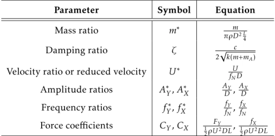
Lw = length of near-wake (only forL2 regime),Lf = length of eddy formation region (fromL3 toT2 regimes),CD Drag coefficient. Abbreviations: ր in-crease,ցdecrease, ↓rapid decrease, (?) unknown. . . 8 2.2 Separation Reynolds number,Res. . . 10 2.3 Reoscaccording to various authors. . . 13 2.4 Principal non-dimentional parameters for the analysis of the flow cylinder
displacement, Blevins (1977); Khalak and Williamson (1999). . . 32
3.1 Gmsh commands used in the meshes generation. . . 41 3.2 Gmsh alternative software to perform mesh generation. . . 44 3.3 OpenFOAM alternative softwares to perform numerical fluid simulation. . . 49 3.4 Specifications of the machine used to performed the Computational Fluid
Dynamics (CFD) simulations. . . 50
4.1 Relation between the fundamental quantities convergence with the discretiza-tion variadiscretiza-tion for meshes with 2500Ddomain length andRe= 200. . . 53 4.2 Relation between the fundamental quantities convergence with the time step
variation for the mesh 1 with 2500Ddomain length andRe= 200. . . 56 4.3 Relation between the flow fundamental quantities convergence with the
do-main length,Lb, andRe= 200. . . 58 4.4 Relation between the fundamental quantities convergence with the
discreti-sation variation for meshes with 8Ddomain length andRe= 200. . . 59 4.5 Comparison of fundamental quantities obtained in this thesis with the data
described in the literature for a flow around a fixed cylinder,Re= 200. . . 60
5.1 Cylinder properties. . . 64 5.2 Flow properties. . . 64 5.3 Simulation parameters for the mass-spring and mass-spring-damping systems
to the cylinder with Y-only motion. . . 64 5.4 Obtained results to mass-spring system to cylinder with Y-only motion. . . . 67 5.5 Obtained results for the mass-spring system for the cylinder with Y-only
5.6 Obtained results to mass-spring-damping system to cylinder with Y-only
mo-tion. . . 85
6.1 Simulation parameters for the cylinder with XY-motion. . . 91
6.2 Geometric parameters of the 8Dmesh. . . 91
6.3 Geometric parameters of the asymmetric 8Dmesh. . . 98
6.4 Geometric parameters for second level of refinement in the 8Dmesh. . . 103
6.5 Fundamental quantities and 8-motion last cycle of the 8Dmesh. . . 104
6.6 Geometric parameters for third level of refinement in the 8Dmesh. . . 108
6.7 Fundamental quantities and 8-motion last cycle of the 20Dmesh. . . 113
6.8 Geometric parameters of the 20Dmesh. . . 114
6.9 Fundamental quantities and 8-motion last cycle of the 500Dmesh. . . 119
6.10 Geometric parameters of the 500Dmesh. . . 120
6.11 Fundamental quantities and 8-motion last cycle of the 2500Dmesh. . . 125
CFD Computational Fluid Dynamics.
DOF Degree Of Freedom.
FFT Fast Fourier transform.
FVM Finite Volume Method.
PIMPLE Pressure-Implicit Method for Pressure-Linked Equations.
PISO Pressure Implicit Splitting of Operators.
SIMPLE Semi-Implicit Method for Pressure-Linked Equations.
δt Time-step
δx Mesh cell size in the direction of the velocity
A
D Adimensional amplitude
D
B Wall blockage parameter
e
D Thickness of the first element along the cylinder wall
ν Kinematic viscosity
ρ Density
ζ Damping coefficient
A Oscillation amplitude
a1 Length of the mesh cell first node
B Distance between two parallel walls of the domain
CA Ideal added mass coefficient
CD,mean Drag coefficient mean
CD,rms Drag coefficient root mean square
CD Drag coefficient
CL,rms Lift coefficient root mean square
CL Lift coefficient
Co Courant number
D Cylinder diameter
f Frequency of vortex shedding
fst Strouhal frequency
k Stiffness
Lf Length of eddy formation region
Lw Length of near-wake
m Mass
m∗ Mass ratio
n Number of radial nodes
Nang Number of elements around the cylinder
Nrad Number of elements in the radial direction
p Local pressure
p∞ Free stream static pressure
r Progression value of the mesh cells
Re Reynolds number
Ro Roshko number
Sn Mesh radial distributed nodes length
St Strouhal number
t Time
Te Cylinder oscillation period
U Velocity magnitude
U∗ Reduced velocity
C
h
a
p
t
1
Introduction
1.1 Context and motivation
Engineering had a decisive role in the development of mankind, contributing to a number of innovations that had enabled the twenty-first century way of life. Constantly struggling with new challenges, engineering is in a permanent search of innovative ap-proaches to address those challenges. Particularly, in terms of mechanical structures, the materials have been stretched more frequently for its mechanical limits. With greater exigency levels, new materials with higher levels of flexibility, strength and lightness have been emerging to meet the demands of increasingly ambitious projects. Similarly, in recent times, many investigations have been motivated by the engineering applications of vibration, such as the design of machines, foundations, structures, engines, turbines, and control systems. The development of these novel technologies is closely related with the understanding of the physical phenomenon that they will be subjected to.
In CFD one of the most studied phenomenon is the flow around a circular cylinder. This phenomenon became a subject of special interest in this area after it was understood that it was not as trivial as thought to the date. In fact, it was realized that involved complex physical aspects and was related with some interesting and particular details, like the development of vortex shedding in unsteady flow, Williamson and Govardhan (2004).
there are a scarce number of articles focusing the numerical simulation of this kind of problem.
These studies are important to better understand how aerodynamic and hydrody-namic environments influence structures fatigue damage and stability. An example of how crucial these studies are, was the collapse of Tacoma Bridge, built in 1940 in the United States of America, Billah and Scanlan (1991). This bridge caved in only two months after its inauguration due to vortex induced vibrations. More specifically, vortex shedding induced the development of vortices on the back side of the bridge. As the wind increased in speed, vortices were formed on alternate sides of the downwind side which, eventually, broke loose and flew downstream exerting fluctuating vertical forces on the bridge even though the wind was blowing across it in a transverse, horizontal direction. The oscillating forces induced by the vortex shedding were increasingly higher with each cycle because the wind energy was higher than the flexing of the structure was able to dissipate and, finally, drove to the bridge failure due to excessive deflection and stress.
Thus, examples of structures subjected to vortex induced vibrations phenomenon are bridges, high-rise buildings, high voltage towers, industrial chimneys, wind turbines, underwater structures, offshore platforms, ship hulls, drilling and production risers in petroleum exploration, pipelines networks such as pipelines or structures involving dif-ferent types of cables like electric networks or suspended structures.
Whenever the natural frequency of vibration of a machine or structure coincides with the frequency of the external excitation, there occurs a phenomenon known as resonance, which leads to excessive deflections and failure, as the one that occurred in Tacoma bridge. Therefore, due to the devastating effects that vibrations can have on machines and structures, vibration testing has become a standard procedure in the design and development of most engineering systems. With this interest comes the need for numerical tools with the power to perform a detailed analysis of this kind of phenomena and, at the same time, affordable enough to perform an efficient study.
In this context, the development of this work aims to validate the numerical code of the OpenFOAMsoftware. This is an open source tool, which is understood to be strong enough for the numerical simulation of a flow around a cylindrical section with two DOF.
1.2 Problem formulation
performed a comparison study between the developed meshes. Comparing its dimension-less parameters values, the simulation performance, and the obtained results with the literature data it was possible to conclude which one of these meshes configurations was the best fit to proceed the analysis of the flow around a cylinder with one and two DOF.
Subsequently, it was studied the VIV phenomena in a circular body with one DOF for a
Y axis motion. For this scenario, it was evaluated the cylinder perpendicular displacement towards the flow direction.
Finally, it was studied the VIV for a circular cylinder with two DOF.
For the three cases enumerated above, the results validation was performed by com-paring the obtained results with the data described in the literature.
1.3 Original contributions
This thesis validates the use of OpenFOAM for the numerical study of a flow around a cylindrical section in the two DOF scenario. The validation of this tool becomes im-portant in the development of the computational fluid dynamics area, as it validates an alternative tool to the traditional, expensive and inaccessible software. Demonstrating that this alternative tool has similar potential but, being open-source, can be easily avail-able to anyone interested in performing this kind of study. Contributing, therefore, for the knowledge to increase in this area which has so many fascinating unexplored subjects.
1.4 Thesis layout
Apart from this introduction, this thesis is structured in six chapters. In chapter 2 are introduced the main theoretical topics related with the phenomena of a flow around a circular cylinder. Furthermore, in section 2.3 are detailed the mathematical equations modelling the flow displacement in CFD.
Chapter 3 describes the numerical modelling methodology used to simulate an un-steady flow around a circular cylinder. Namely, it is described the mesh generation process in section 3.1 and specified how the CFD analysis was set using OpenFOAM in section 3.2.
Then, in chapter 4 the CFD study of a flow around a non-oscillatory cylinder. Particu-larly, in section 4.1 is done a mesh independence study.
Afterwards, in chapter 5 it is studied a flow around a cylinder with one DOF. Particu-larly, it was performed an analysis for the mass-spring system in subsection 5.1.1 and for the mass-spring-damping system in subsection 5.1.2.
C
h
a
p
t
2
Theoretical contextualization
2.1 Fundamentals of a flow around a circular cylinder
A fluid flow around a stationary body or, similarly, a movement of a body in a fluid at rest originates a region of disturbed flow at the body boundaries. The extension of the affected region is largely influenced by the body shape, orientation and size and by the fluid velocity and viscosity. This relation is translated by the Reynolds number,Re, which is a dimensionless parameter that depends on the fluid density,ρ, velocity,U∞, cylinder external diameter which corresponds to the body characteristic length,D, and dynamic viscosity,µ.
Re=ρU∞D
µ (2.1)
Bodies subjected to a fluid flow are classified as being streamlined or bluff, depending on their overall shape. Particularly, in this thesis context, we are interested in the interac-tion between a bluffstructure and a subsonic flow. Bluffbodies are characterized by flow separation along a large section of the structure’s surface, Bearman (1984). The primary purpose of these structures is to bear loads, contain flow or provide heat transfer structure and, since these structures are not designed to minimize drag, aerodynamic optimization is not usually a concern. Consequently, flow induced vibrations are generally considered as a secondary design parameter, at least until a failure occurs.
Kármán street. Circular cross-section bodies such as cylinders are classified as bluff bodies since, as a result of its shape, generate particularly large and typically unsteady flow separation structures.
2.1.1 Disturbed regions in a circular cylinder
The flow disturbed regions are defined by the variation of its velocity magnitude, direction and time. In each region the disturbed flow is characterized by a greater, equal or minor velocity than the free stream velocity, Zdravkovich (1997). Figure 2.1 illustrates the flow different disturbed regions:
i. narrow region of retarded flow;
ii. boundary layers attached to the surface of the cylinder;
iii. sidewise regions of displaced and accelerated flow;
iv. wide downstream region of separated flow designated by the wake.
Figure 2.1:Disturbed flow regions, Zdravkovich (1997).
2.1.2 Transition in disturbed regions
The flow transition from laminar to turbulent state is given by the Reynolds number,
Re, which represents the ratio between inertial and viscous forces defined by equation 2.1.
Laminar flow occurs for low Reynolds numbers, where viscous forces are dominant, and is characterized by smooth, constant fluid motion. Oppositely, turbulent flow occurs for high Reynolds numbers and is dominated by inertial forces, which tend to produce flow instabilities such as vortices.
Figure 2.2:Transitions in disturbed regions: (a)T rW, (b)T rSL, (c), (d)T rBL(BL=boundary layer, L=laminar, T=turbulent, Tr=transition, S=separation), Zdravkovich (1997).
The first disturbed region, designated by T rW, occurs in the wake and gradually spreads along it while the free shear layers bordering the near-wake remain laminar. The second transition, represented byT rSL, occurs in the free shear layers. This transition is characterized by the increasing of the Reynolds number along the free shear layers towards the separation and impacts the length and weight of the near-wake. For the third transition, T rBL, the flow is turbulent in the free-shear-layers and the remaining flow is in a transition state. The third transition is considered to be completed when all the regions of disturbed flow are fully turbulent. At this point, the stagnation point, where the fluid local velocity is zero, and the separation point, where the wall shear stress is equal to zero, are coincident.
2.1.3 Types of the flow states
The flow around a circular cylinder is an extremely complex phenomenon. Neverthe-less, flow patterns are expected to be confined within a fixed range ofRefor genuinely disturbance free flows, Zdravkovich (1997).
The flow states can be fully laminar, L, one of the three transitions T rW, T rSL or
T rBL, or fully turbulent,T. Each flow state can be described in a flow regime context depending on the Reynolds number. Table 2.1 enumerates the flow regimes for a flow around a circular cylinder.
The Reynolds number considered for the simulations developed in this work corre-sponds toRe= 200. For this reason, in the next subsections will be discussed theLand
T rW flow regimes, the existent regimes untilRe= 200. The remaining flow states and flow regimes will not be discussed in detail in this work, since they are not relevant in this thesis context.
2.1.3.1 Laminar state of flow,L
The laminar state of flow can be divided into three basic flow regimes:
L1 : "Creeping" flow or non-separation regime; 0< Re <4 to 5
L2 : Steady separation or closed near-wake regime; 4 to 5< Re <30 to 48
Table 2.1:Disturbance-free flow regimes around a circular cylinder, Zdravkovich (1997). Lw =
length of near-wake (only forL2 regime),Lf = length of eddy formation region (fromL3 toT2
regimes), CD Drag coefficient. Abbreviations: ր increase, ցdecrease, ↓rapid decrease, (?)
unknown.
State Regime ReRanges Lw
Lf CD
L Laminar
1 No-separation 0 to 4-5 None ց
2 Closed wake 4-5 to 30-48 ր ց
3 Periodic wake 30-48 to 180-200 ց ր
T rW Transition
in wake
1 Far-wake 180-200 to 220-250 ց ր 2 Near-wake 220-250 to 350-400 ր ց
T rSL Transition in
shear layers
1 Lower 350-400 to 1k-2k ր ց
2 Intermediate 1k-2k to 20k-40k ց ր 3 Upper 20k-40k to 100k-200k ց ր
T rBL Transition in
boundary layers
0 Pre-critical 100k-200k to 300k-340k ր ց 1 Single bubble 300k-340k to 380k-400k (?) ↓ 2 Two-bubble 380k-400k to 500k-1M (?) ↓ 3 Supercritical 500k-1M to 3.5M-6M None ր 4 Post-critical 3.5M-6M to (?) (?) ր
T Fully turbulent 1 Invariable (?) to∞ (?) ր
2 Ultimate (?) to∞ (?) (?)
2.1.3.1.1 "Creeping" flow,L1
The "creeping" flow regime occurs for low Reynolds values and is dominated by vis-cous forces to such an extend that all disturbed regions remain laminar, as figure 2.3 shows. The creeping flow, L1, past a cylinder persists without separation up toRe≃5, Camichel and Escande (1938).
Figure 2.4 shows the streamlines and three velocity profiles superimposed at stations
−8D, 0, and 8D. The retarded region of flow is very large, being almost 20D wide at the upstream station−8D. The thick shear layers displaced by the cylinder are not sur-rounded by the accelerated region as illustrated in figure 2.1. The sidewise divergence of all streamlines in figure 2.4 prevents the increase of velocity throughout the visible flow field. The velocity deficit at 8Ddownstream at the wake axis is around 50%. The cylinder is "pushing" and "dragging" a 20Dwide trail by the action of large viscous forces.
Figure 2.3:Creeping flow forRe= 1, Camichel and Escande (1938).
Figure 2.4:Flow field around a stationary circular cylinder atRe= 3.5, Wieselsberger (1921).
The velocity field around a circular cylinder at lowReis associated with the charac-teristic pressure distribution around the cylinder. The measured pressure is expressed in a non-dimensional parameter designed by pressure coefficient:
Cp=p1−p∞ 2ρV2
(2.2)
wherepis the local pressure on surface,p∞is the free stream static pressure and12ρU2 is the free stream dynamic pressure. The circumferential angle is usually measured from the stagnation point, whereθ= 0◦up to 180◦.
A favourable pressure gradient extends untilθ= 115◦atRe= 3.5 followed by a very small adverse pressure gradient that is insufficient to induce separation.
because the size of the near-wake is small and the separation occurs in a region where the velocity is also very small. Nisi and Porter (1923) observed this separation by using smoke visualization and noted the strong effect of the blockage onRes. In table 2.2 are enumerated some estimatedRes values and the respective wall blockage parameter, DB, whereDcorresponds to the cylinder diameter andBto the distance between two parallel walls of the domain.
Table 2.2:Separation Reynolds number,Res.
Authors DB Res
Nisi and Porter (1923) 4.3
Homann (1936) 0.067 6.0
Taneda (1956) 0.01 5-6
Coutanceau and Bouard (1977)
0.12 9.6
0.07 7.2
0.00 4.4
2.1.3.1.2 Steady separation regime,L2
ForRe >4−5, starts a new laminar flow regime. This flow regime occurs untilRe <
30−48 and is characterized by the development of a steady region confined in a closed and symmetric near-wake, marked by a noticeable change in pressure distribution. As it is possible to conclude from figure 2.5, the separation of the shear layers merge the wake and make a symmetric, steady and closed near-wake.
Figure 2.5:Steady closed near-wake atRe= 23, Thom (1933).
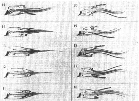
of a new near-wake is accomplished by a secondary separation of the free shear layers from the near-wake, phenomena illustrated in images 4, 5 and 6. In image 9 is shown the approximation and, finally, the merge of the separated shear layers. The last image, image 10, shows the steady near-wake atRe= 40.
Figure 2.6:Metamorphose of near wake withRebetween 20 and 40, Camichel et al. (1927).
2.1.3.1.3 Periodic laminar regime,L3
The steady, elongated and closed near-wake becomes unstable whenRe > Reosc, which occurs forRe >30−48. The transverse oscillation begins at the end of the near-wake and initiates a wave along the trail as shown in figure 2.7, Homann (1936). The maximum adverse gradient also occurs around the confluence point at the near-wake end, where the instability starts. The coincidence between the location of the instability and the adverse pressure gradient suggests their correlation.
Figure 2.7:Begin of oscillating wake forRe= 54, Homann (1936).
Taneda (1956) called the spiky ends in figure 2.8 by "gathers". He stated that "the gathers first appear forRe >35 near the downstream end of the near-wake border-line, move towards the rear end of the near-wake, tremble there for a while and die away". Also, he referred that the trail began to oscillate sinusoidally before the gathers were formed, meaning that the former induced the latter. Contrary to that, Gerrard (1978) observed that the periodic appearance of gathers resulted in a wavy trail.
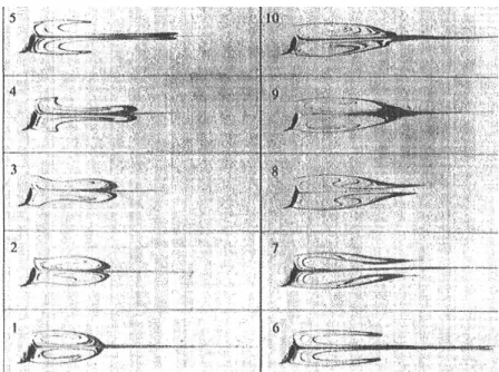
Figure 2.8:Development of near-wake oscillation with the increase ofRefrom 30 to 60, Camichel et al. (1927).
Figure 2.8 illustrates the near-wake oscillation with the increase ofRefrom 30 to 60 from image 11 to 20, respectively. Analysing figure 2.8, is visible a gradual reduction in length of the closed near-wake from Lw
D = 3.5 to 2 and a continuous increase in amplitude of oscillation at the end of the near-wake from 0 to 12D, whereLw represents the wake length and D the cylinder diameter. Nishioka and Sato (1978) found a gradual and continuous reduction of Lw
D for 40< Re <120 while Gerrard (1978) reported a sudden shrink between 60< Re <70.
There is a wide range of reported Reosc values at which the near-wake instability initiates even when the blockage is negligible. The flow visualisation data tend to be on the lower side and hot-wire anemometry measurements on the higher side as shown in table 2.3. The latter may be due to insensitivity of a single hot wire to a periodic change in velocity direction. Furthermore, Kovasznay (1949) reported thatReosc did not show a hysteresis effect, this means that the same value was found when increasing or decreasing the velocity magnitude.
The instability of the near-wake begins when Re > Reosc. Also, when the blockage effect is negligible, some disparity is observed in the obtained results for theReosc values between some authors, as it can be observed in table 2.3.
Table 2.3:Reoscaccording to various authors.
Method Author(s) Reosc
Flow visualization
Taneda (1956) 30
Coutanceau and Bouard (1977) 34
Gerrard (1966) 33
Hot-wire anemometry
Kovasznay (1949) 40
Roshko (1954a) 40
Nishioka and Sato (1978) 48
dimensionless parameter which describes oscillating flow mechanisms. This parameter was later designed by the Strouhal number:
St=f D
U (2.3)
wheref is the frequency of vortex shedding,Dis the characteristic length of the cylinder andUis the free stream velocity.
Zdravkovich (1985) adapted from Strouhal the measured variation ofStin terms of
Re, fact illustrated in figure 2.9.
Figure 2.9:St−Rerelationship non-linear in the laminar periodic regime,L3, Zdravkovich (1985).
Roshko (1954b) suggested a new dimensionless parameter, whereνcorresponds to the kinematic viscosity:
Ro=f D 2
ν (2.4)
that makes the following linear relationshipRo−Re:
this linear relation between the eddy frequency and the velocity is illustrated in figure 2.10 and can be used to measure very low velocity values.
Figure 2.10:Roshko’s number variation in terms ofRe, Zdravkovich (1997)
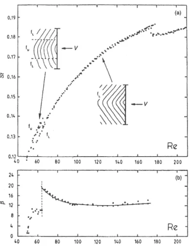
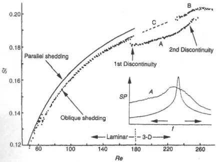
Tritton (1959) discovered that forRe= 80 existed a discontinuous drop in shedding frequency using Roshko’s relationship. Nevertheless, surprisingly he also discovered that the drag coefficient was not affected by this discontinuity. Williamson (1988, 1989) re-solved this enigma when he proved that the discontinuity was caused by the transition from one slanted shedding mode to another slanted mode. Figure 2.11 shows the simul-taneous measurements of the angle of the slanted eddy filament, β, and the Strouhal number,St, in terms ofRe.
Williamson (1989) proved that the parallel shedding mode is the universal one. Any slanted eddy shedding, St, could be transformed into the universal mode Stu, by the trigonometric relation given by equation 2.6.
Stu=Stcos(β). (2.6)
2.1.3.2 Transition-in-wake state,TrW
All laminar flows eventually become unstable above a certainReand undergo transi-tion to turbulent. The flow in a wake does not become fully turbulent as soon as it ceases to follow the laws of laminar flow. This transformation occurs in a finite transition region characterized by the random initiation and growth of irregularities. Furthermore, the viscous diffusion and mutual interaction of laminar eddies add a greater complexity to the periodic laminar wakes transition.
Figure 2.11:Effect of number of end cells onSt, Williamson (1988, 1989).
T rW1 Lower transition regime, where the eddies are formed laminar and regular but become irregular and transitional downstream.
T rW2 Upper transition regime, where the eddies are formed laminar and irregular but become partly turbulent before they are shed and carried downstream.
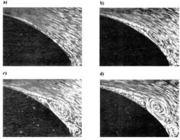
Peculiar distortions of the laminar filaments adjacent to the cylinder are shown in figure 2.12. The development of these structures occurs when a flow in laminar state is close to the transition state. This phenomenon is related with distortions that are typically formed in the laminar eddy filaments at this point. These distortions were designated by fingers by Gerrard (1978) because they pointed towards the cylinder. Illustrated in figure 2.12 are two types of fingers, a finger of type A atRe= 180 and a second finger of type B atRe= 230.
Figure 2.12:Consecutive formation of fingers,Re= 180, Gerrard (1978).
modes of eddy shedding. Roshko (1954c) repeated measurements of shedding frequency in a large low-turbulence wind tunnel and proposed the following ranges:
i. Stable range, 40< Re <150, regular velocity fluctuations and risingSt.
ii. Unstable range, 150< Re <300, irregular bursts in velocity fluctuations,Stunstable.
iii. Irregular range,Re >300, irregular and periodic,Stis constant.
The figure 2.13 shows a particularly large scatter of experimental points in theT rW
regime. The boundary betweenT rW1 andT rW2 is marked by a jump inStatRe≃250 which separates risingStfromSt=constant.
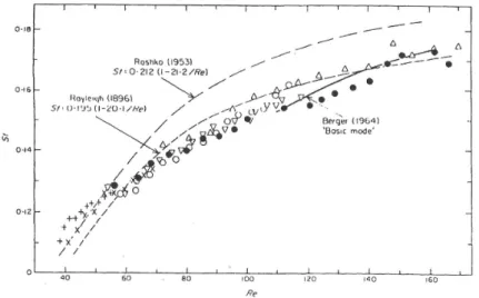
Figure 2.13:Variation ofStin terms ofRe, Roshko (1954c).
Roshko suggested two empirical relations:
St= 0.212(1−21.2
Re ) forRe <180 St= 0.212(1−12.7
Re ) forRe >300
The two differentStcurves correspond to two different modes of eddy shedding. Kovasznay (1949) noted that laminar eddies are not shed from the cylinder but rather formed gradually as they are carried downstream. He attributed this low-speed mode to the instability of the laminar wake. As an example of the low-speed mode, figure 2.14(a) shows the laminar periodic wake atRe= 140, which illustrates that all eddies are mutually connected by the trail streak-line originated in the near-wake. Figure 2.14(b) exhibits the salient features of high-speed mode at Re= 300 in T rW2 regime. In this figure the trail streamline is not seen and that means that the eddies are not mutually connected.
Figure 2.14:(a) Laminar periodic wake atRe= 140; (b) transitional periodic wake atRe= 300, Freymuth (1985).
In Zdravkovich (1997) it was refereed the existence of two discontinuities in theSt−Re
relationship. Figure 2.15 shows a risingSt up to the first discontinuity atRe= 170. A narrow frequency peak is showed in figure 2.15 whenReincreases and a wide frequency peak at a slightly lower value ofSt whenRedecreases. A possible explanation for the lower value of St when Re decreases, is the occurrence of the hysteresis effect in the fingers formation. The second discontinuity inStoccurs between, 225< Re <270. Two suggestions were made to explain this. The first was provided by Williamson (1989) who proposed that they do not coexist simultaneously. The other suggestion was presented by Zdravkovich (1992) who affirmed that the two peaks represent the overlapping of two modes of eddy shedding, and both may exist simultaneously.
2.1.4 Vortex shedding and vortex patterns
Figure 2.15:Variation ofSt in terms ofRe. Insert: frequency spectra atRe= 172, Zdravkovich (1997).
alternated vortex shedding release, as shown in figure 2.16. When the pressure field is maximum in the cylinder top, the flow is accumulated in the bottom side. As the bottom side of this flow accumulation has a higher flow velocity, because it is in contact with the flow free stream, and the top side of the flow accumulated is in cylinder aft and has a lower velocity flow, the flow tends to whirl developing, this way, a vortex. The detach-ment of the vortex is triggered by the pressure field displacedetach-ment to the bottom side of the cylinder. When the pressure field arrives the bottom side, pushes the vortex, slitting the connection between the vortex and the cylinder. When the vortex is released, moves in the wake, being gradually elongated and expanded. The vortex is finally dissipated when its pressure evens the free stream velocity. This process is repeated while the fluid flows around the circular cylinder corresponding each vortex released to a cycle in the alternated vortex shedding, Blevins (1977). The detail of the vortex development in the cylinder boundary wall is shown in figure 2.17.
The development of the vortex shedding phenomenon induces the creation of several forces which promote the cylinder oscillation. This forces are designated by lift force and drag force. Particularly, the lift force is the force caused by the interaction between the fluid and the structure, in the problem studied in this thesis corresponds to the force ap-plied in the cylinder in the transversal direction towards the flow displacement direction. As the name indicates, corresponds to the force which is able to sustain the body by the flow displacement, overcoming the gravity force that the body is also subjected too. In the other hand, the drag force is the force generated by the interaction between the body and the fluid in the parallel direction to the fluid motion direction. It represents the force that the body needs to overcome to be able to move through the fluid.
Figure 2.16:Representation of one third of one cycle of vortex shedding of the oscillation sequence of pressure field inRe= 1.12×10⁵, Blevins (1977).
Figure 2.17:Vortex formation near to the cylinder, Mayes et al. (2003).
lift and drag by their one-dimensional quantities, lift coefficient and drag coefficient. Equations 2.8 and 2.9 represent the lift and drag coefficient, respectively. Regarding the lift coefficient,CL, FL represents the lift force and for the drag coefficient, CD, FD represents the drag force. Common to both coefficients,ρrepresents the density,Dis the body diameter andU∞is the value of the free stream velocity.
CL= 1 FL 2ρDU∞2
(2.8)
CD = 1 FD 2ρDU∞2
2.1.5 Response modes for a cylinder with one-degree-of-freedom in transverse motion, Y-only
A high attention has been given to studying the flow around the oscillating cylinder with one DOF, in Y-only motion (transverse to the flow motion). An example of that is the work developed by Bearman (1984) and Sarpkaya (1979). A flow around a circular cylinder creates a fluctuating lift force, transverse to the flow direction caused by the alternating vortex shedding, inducing the vibration of the structure. One of the main characteristics of flow-induced vibration is the ability of the vibration originated by the vortex shedding to be synchronized with the natural frequency, (fn), of the structure. The occurrence of this phenomenon during a long period of time can lead to the structure collapse.
In the case of a cylinder oscillating transversely to the free stream, the relevant dimen-sionless parameters in addition to the Reynolds Number, which was already presented in section 2.1.1, is the oscillation amplitude, Aand the frequency,fe (or the periodTe). However, it is common to use the wavelength which corresponds to the sinusoidal path along which the body travels relative to the fluid. Therefore, the relevant parameters are:
Amplitude ratio= A
D (2.10)
W avelength ratio=UTe
D = λ
D (2.11)
whereU is the velocity in thex-direction, andTe is the cylinder oscillation period in the transverse direction. The normalized wavelength is equivalent to what is usually referred to as reduced velocity.
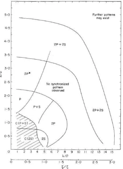
Williamson and Roshko (1988) studied the vortex wake patterns for a cylinder, trans-lating in a sinusoidal trajectory, over a wide range of amplitudes and wavelengths. They defined a whole set of different regimes for vortex wake modes, using controlled vibra-tions, in the plane of (λ/D,A/D). With this, Williamson and Roshko created a map which standardized the vortex shedding with the oscillation of the cylinder withY-only motion in the plane (λ/D,A/D). These authors also defined nomenclatures for each vortex wake mode. The terminologyP was assigned when a vortex pair was released in each peak of the cylinder oscillation and the terminology S was attributed when a unique vortex was released in each peak of the cylinder oscillation. In figure 2.18 are represented the different types of vortex pattern shedding for each cycle defined by these authors.
Figure 2.19 displays the map created by Williamson and Roshko. Analysing this figure, it is possible to observe the map with the different zones corresponding to the vortex pattern shedding into the cylinder transversely to the flow in function of the oscillation amplitude and wavelength.
The most important patterns of vortex shedding are represented by 2S, 2P andP+
designation means it is released a vortex pair for each peak in the amplitude of the cylinder oscillation, and the designationP+Smeans that is released a vortex pair in the oscillation peak with another single vortex released in the symmetric peak, forming a vortex pattern shedding according to asymmetric vortex swing by the cylinder axis of symmetry. Other patterns are denoted by C(2S) andC(P+S), which means that close to the cylinder are formed 2S andP+S vortex pattern shedding but these vortex are small and are joined immediately behind the cylinder. The regions denoted byP and 2P∗
are referred to as the "single pair" and "double pair" by Williamson Williamson (1985). Finally, the vortex pattern defined by 2P+ 2Scompress two vortex pairs formed during one oscillation cycle in the two cylinder peaks but with the release of a vortex cylinder each time through the movement of the axis of symmetry. The part of the (λ/D, A/D) plane in figure 2.19 which has no nomenclature associated corresponds to regions where no periodic synchronized mode of vortex formation was observed by Williamson and Roshko.
2.1.6 Response modes for a cylinder with two-degrees-of-freedom in
XY-motion
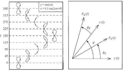
The cylinder 8-motion is characterized by the relation between the lift and drag forces. Throughout the development of the phenomenon, i.e., the oscillation of the pressure field and the variation of the lift and drag forces causing the release of vortices in the cylinder back, the intensity of drag and lift forces vary, causing the cylinder movement along theX
andY axis, respectively. The existence and interaction of both these forces are the reason why a cylinder with two DOF describes a movement in an eight conformation. There are several types of 8-motion which are influenced by the phase in which the lift and drag forces are. Figure 2.20 illustrates the movement’s dependence on the phase in which the drag and lift forces are, showing a set of possible 8-motions.
Figure 2.20: Map of vortex synchronization regions in the wavelength-amplitude (λ/D, A/D) plane, Williamson and Roshko (1988).
Contrarily to the high attention given to the study of the flow around an oscillating cylinder with one DOF, transverse to the flow direction, there are seldom studies pub-lished about the oscillating cylinder with two DOF. Thus, one of the most interesting subject between these two movement types, theY-only motion andXY-motion, that still holds is:
What differences exist between a flow around a cylinder with one DOF transversely to the flow and a flow around a cylinder with two DOF?
Furthermore, Jauvtis and Williamson (2003) also asked a key question,
To what extend are these transverse response modes and amplitudes influenced by the body’s freedom to respond in the streamwise direction?
They feature comparison of the cylinder amplitudes, for movements inX andY, and the frequency,fY, in relation to the reduced speed,U∗which is similarly defined in table 2.4. These values are illustrated in figure 2.21.
Figure 2.21:Transverse and streamwise amplitudes (A∗Y andA∗X) and frequency (fY∗) response in function of the reduced velocity (U∗) for moderate mass ratios,m∗= 7.0. Solid symbols correspond
toY-only data and open symbols toXYdata.Re= 2000−11000. Jauvtis and Williamson (2003).
Interestingly, as shown in figure 2.21, the response differences between a cylinder in a one DOF and in a two DOF conformation are not very significant even for low mass value ratio,m∗= 6.9, and low mass damping (m∗+C
A set of amplitude peaks of the upper and lower branches, were also measured by Jau-vtis and Williamson (2003) as illustrated in figure 2.22, depending on the mass damping parameter (m∗+CA)ζ. The only change noted in the response amplitude between the two movements was between the range of values of the mass damping (m∗+C
A)ζ= 0.01−0.1 and between the range of values of the mass ratiom∗= 5.0−25.0. The figure 2.22 shows
the transverse amplitude with the mass-damping parameter.
Figure 2.22:Griffinplot of the transverse amplitude peak variation (A∗
Y max) with the combined
mass-damping parameter (m∗+C
A)ζ, for moderate mass ratios,m∗= 6−25. Jauvtis and Williamson
(2003).
Jauvtis and Williamson (2003) shows that for lower mass ratios, m∗<6, exists a
re-markable jump that increases the amplitude of cylinder response, corresponding to a new mode of cylinder response, which is quite distinct from the response phenomena in Y-only motion.
The first evident difference regarding the amplitude response is the remarkably high amplitude, about A∗Y = 1.5. For this high amplitude of the cylinder response with 2 DOF, Jauvtis and Williamson (2003) define this as the "super-upper" branch of response, different from the "upper" branch observed in the Y-only motion.
The figure 2.23 shows the cylinder response with two DOF for reduced velocity values betweenU∗= 2−13.5 observed in Jauvtis and Williamson (2003). Also, in Jauvtis and
Williamson (2003) it are described the several branches of the cylinder response.
Following the results shown in figure 2.23, in figure 2.24 it is possible to observe the 8-motion types detected by Jauvtis and Williamson (2003) as the reduced velocity increases for lower values of reduced mass.
Figure 2.23:Transverse and streamwise amplitudes (A∗
Y andA∗X) and frequency (fY∗) response in
function of the reduced velocity (U∗) for low mass ratios,m∗= 2.6. Solid symbols correspond to Y-only data and open symbols toXYdata.Re= 2000−11000. Jauvtis and Williamson (2003).
Re= 330−15300. About the super-upper and lower branch levels of peak response Jauvtis and Williamson (2003) said apparently are independent of the Reynolds number for this range investigated by Jauvtis and Williamson (2003).
Interestingly, Jauvtis and Williamson (2003) observed that when the mass ratio is gradually reduced at a fixed mass-damping, the peak of the transverse amplitude is not affected and remains at the value of the upper branch. This occurs until the mass ratio of
m∗= 6, from which the streamwise amplitude starts to increase, asm∗is further reduced.
Figure 2.24:Transverse and streamwise amplitudes (A∗
Y andA∗X) and frequency (fY∗) response in
function of the reduced velocity (U∗) for low mass ratios,m∗= 2.6. Solid symbols correspond to Y-only data and open symbols toXYdata.Re= 2000−11000. Jauvtis and Williamson (2003).
2.2 Fundamentals of Vibration
Any motion that repeats itself after an interval of time is called vibration or oscillation. The theory of vibration deals with the study of oscillatory motions of bodies and the forces associated with them. A vibratory system, in general, includes the means for storing potential energy (spring or elasticity), the means for storing kinetic energy (mass or inertia), and the means by which energy is gradually lost (damper).
The vibration of a system involves the transfer of its potential energy to kinetic energy and of kinetic energy to potential energy, alternately. If the system is damped, some energy is dissipated in each cycle of vibration and must be replaced by an external source if a state of steady vibration is to be maintained. However, in practice, the magnitude of oscillation (u) gradually decreases and the pendulum ultimately stops due to the resis-tance (damping) offered by the surrounding medium (for instance air). This means that some energy is dissipated in each cycle of vibration due to damping by the air.
Figure 2.25:Griffinplot of the transverse amplitude peak variation (A∗
Y max) with the combined
mass-damping parameter (m∗+C
A)ζfor low mass ratios,m∗ = 2.5−4. Jauvtis and Williamson
(2003).
• Free Vibration: if a system, after an initial disturbance, is left to vibrate on its
own, the ensuing vibration is known as free vibration. No external force acts on the system. The oscillation of a simple pendulum is an example of free vibration.
• Forced Vibration: if a system is subjected to an external force (often, a repeating
type of force), the resulting vibration is known as forced vibration. The oscillation that arises in machines such as diesel engines is an example of forced vibration. If the frequency of the external force coincides with one of the natural frequencies of the system, a condition known as resonance occurs, and the system undergoes dangerously large oscillations. Failures of such structures as buildings, bridges, turbines, and airplane wings have been associated with the occurrence of resonance.
• Undamped vibration: if no energy is lost or dissipated in friction or other resistance
during oscillation, the vibration is known as undamped.
• Damped vibration: if some energy is lost in friction or other resistance during
os-cillation, the vibration is called damped vibration. In many physical systems, the amount of damping is so small that it can be disregarded. However, considera-tion of damping becomes extremely important in analysing vibratory systems near resonance.
vibration. The differential equations that govern the behaviour of linear and non-linear vibratory systems are linear and non-linear, respectively. If the vibration is linear, the principle of superposition holds, and the mathematical techniques of analysis are well de-veloped. For non-linear vibration, the superposition principle is not valid, and techniques of analysis are less well known. Since all vibratory systems tend to behave non-linearly with increasing amplitude of oscillation, a knowledge of non-linear vibration is desirable in dealing with practical vibratory systems.
If the value or magnitude of the excitation (force or motion) acting on a vibratory system is known at any given time, the excitation is called deterministic. The result-ing vibration is known as deterministic vibration. In some cases, the excitation is non-deterministic or random and, for these situations, the value of the excitation at a given time cannot be predicted. In these cases, a large collection of records of the excitation may exhibit some statistical regularity. It is possible to estimate averages such as the mean and mean square values of the excitation. Examples of random excitations are wind velocity, road roughness, and ground motion during earthquakes. If the excitation is random, the resulting vibration is called random vibration. In this case the vibratory response of the system is also random and it can only be described in terms of statistical quantities.
Regarding the damping elements, viscous damping is the most commonly used damp-ing mechanism in vibration analysis. When mechanical systems vibrate in a fluid medium such as air, gas, water, or oil, the resistance offered by the fluid to the moving body causes energy to be dissipated. In this case, the amount of dissipated energy depends on many factors, such as the size and shape of the vibrating body, the viscosity of the fluid, the frequency of vibration, and the velocity of the vibrating body. In viscous damping, the damping force is proportional to the velocity of the vibrating body.
2.2.1 Two-Degree-of-Freedom Systems
Usually, the mass, spring and damper do not appear as separate components but as an inherent and integral part of the system. For example, in an airplane wing, the mass of the wing is distributed throughout the wing. Also, due to its elasticity, the wing undergoes noticeable deformation during flight so that it can be modelled as a spring. In addition, the deflection of the wing introduces damping due to relative motion between components such as joints, connections and support as well as internal friction due to micro-structural defects in the material.
Assuming that the motion of the instrument is confined to theXY-plane, the system can be modelled as a massmsupported by springs in theXandYdirections, as figure 2.26 illustrates. Thus the system has one-point massmand two degrees of freedom, because the mass has two possible types of motion: translations along theX andY directions.
Figure 2.26:Schematic diagram ofXY-motion in a spring-mass-damping system.
There are two equations of motion for a two DOF system, one for each degree of freedom. They are, generally, in the form of coupled differential equations and each equation involves all the coordinates. If a harmonic solution is assumed for each co-ordinate, the equations of motion lead to a frequency equation that gives two natural frequencies for the system. With the appropriate initial excitation, the system vibrates at one of these natural frequencies. During free vibration at one of the natural frequen-cies, the amplitudes of the two degrees of freedom are related in a specific manner and the configuration is called a normal mode, principal mode, or natural mode of vibration. Thus, a two DOF system has two normal modes of vibration corresponding to the sys-tem two natural frequencies. If we give an arbitrary initial excitation to the syssys-tem, the resulting free vibration will be a superposition of the two normal modes of vibration. Nevertheless, if the system vibrates under the action of an external harmonic force, the resulting forced harmonic vibration occurs at the frequency of the applied force. Further-more, under harmonic excitation the amplitudes of the two coordinates will be maximum when the forcing frequency is equal to one of the natural frequencies of the system. This phenomenon is designated by resonance.
The configuration of a system can be specified by a set of independent coordinates such as length, angle, or some other physical parameters. Any such set of coordinates is called generalized coordinates. Although the equations of motion of a two DOF system are generally coupled so that each equation involves all the coordinates, it is always possible to find a particular set of coordinates such that each equation of motion contains only one coordinate. The equations of motion are then uncoupled and can be solved independently of each other. Such a set of coordinates, which leads to an uncoupled system of equations, is termed principal coordinates.