Exfoliation in Bags
Using Sonication for
Nanomaterials Synthesis
Dissertation submitted in partial fulfillment of the requirements for the degree of
Master of Science in
Chemical and Biochemical Engineering
Advisor: David Fernández Rivas, Assistant Professor, University of Twente
Co-advisor: Pedro Simões, Assistant Professor,
Faculdade de Ciências e Tecnologia da Universidade Nova de Lisboa
Examination Committee
Chairperson: Ana Aguiar Ricardo, Full Professor, FCT-UNL Members: Isabel Ferreira, Associate Professor, FCT-UNL
Pedro Simões, Assistant Professor, FCT-UNL
Using Sonication for Nanomaterials Synthesis
Copyright c Filipe Gonçalo Jacinto Gomes, Faculty of Sciences and Technology, NOVA
University of Lisbon.
The Faculty of Sciences and Technology and the NOVA University of Lisbon have the right, perpetual and without geographical boundaries, to file and publish this dissertation through printed copies reproduced on paper or on digital form, or by any other means known or that may be invented, and to disseminate through scientific repositories and admit its copying and distribution for non-commercial, educational or research purposes, as long as credit is given to the author and editor.
This document was created using the (pdf)LATEX processor, based in the “unlthesis” template[1], developed at the Dep. Informática of FCT-NOVA [2].
Firstly I would like to thank Professor David Fernández Rivas for his never ending and always present support, for his teachings, his kindness and help in completing this thesis. I would also like thank Bram Verhaagen, as well as Professor David, for the opportunity to closely collaborate with their start-upBuBclean.
To all the people at the UT who made this work possible through their help on the vari-ous scientific methods used. Thank you Dr. Tibor Kudernac, Richard Egberink, Marcel de Bruine, Mark Smithers, Rico Keim, Gerard Kip, Aufried Lenferink, Cees Otto, Sonia Blanco, Frans Segerink, Robert Wijn, Mark Hempenius and the POF research group for making their lab and equipment accessible for me.
A special appreciation to Stefan Schlautman for making it easier to pass the afternoons at the office and for allowing me to share his and Prof. David’s office during my stay at the University of Twente. To Prof. Gardeniers, Peter, Henk-Willem, Pieter, Ilse, Julie, Yuyan, Sebastiaan, Thijs, Hoon, Jöel all the remaining MCS research group, for the friendly welcome, availability in helping with any doubts, the amazing pop-quizz night at the Molly Malone, the kart race and the farewell dinner.
I am also thankful to the Science and Technology Faculty of the University of Twente for their openness to international students. To the various organisations which were critical for an easy integration, ESN, Kick-in, Buddy Program... And to the people I met at the UT who created a friendly atmosphere away from home, which surely eased the stress of writing a thesis.
A special thanks to Professor Carlos Lodeiro Espiño, for allowing this agreement between both Universities and so giving me this opportunity.
To all my family who besides all the distance were surely wishing for my greatest success and worrying for my safe return. To all my friends who I missed a lot during these six months. A special word of appreciation for Vasco for traveling all the way to Amsterdam when I needed his friendly presence and wise words like never before.
Lastly, I must thank João Paulo for his advice, which never left my mind through out these five years of studies.
With the discovery of the amazing properties of graphene a wide range of applications were devised for this material. Due to the foreseeable great demand for graphene, new materials with similar properties, cheaper and of wider availability had to be studied. Molybdenum Disulfide, MoS2, is one of the members of the transition metal dichalcogenides. When this material is in a single-layer disposition it presents very interesting properties for optical and electronic applications. Many of those applications complement areas where graphene is not useful. However, to obtain the MoS2 mono-layers it is necessary to exfoliate this material. Currently the available exfoliation procedures lack the simplicity and the desired scalability for industrial porpuses.
With this project is attempted to use theBuBclean Cavitation Intensifying Bags or CIBs to exfoliate MoS2. The applicability of plain bags and bags with pits will be tested, as well as to which ultrasonic equipment better suits for this new setup. Understanding what cavitation effects cause the material exfoliation is another objective of this project. For that, the mechanical and chemical effects from cavitation will be isolated and the different results compared. In an important analysis will be studied if theBuBclean CIBs are prepared to sustain the intense effects from cavitation.
It was verified that the bags with pits generate very intense cavitation slightly damaging the obtained layers of MoS2. The plain bags showed better yields as well as less damaged flakes. The mechanical effects from cavitation proved to be the main factor in the exfolia-tion process, but lead to the formaexfolia-tion of damaged flakes in the long run. The chemical effects on their own, manage to produce some exfoliated MoS2. TheBuBcleanCIBs showed proper resistance to cavitation but also leaked when the temperature in the bath increased with time. Further studies must be done to understand if this is viable upgrade to the exfoliation process.
Keywords: Exfoliation - Molybdenum Disulfide - Cavitation - BuBclean CIB
Com a descoberta das propriedades inigualáveis do grafeno surgiram um enorme número de aplicações para este material. Devido à expectável procura por este material, novos ma-teriais de propriedades semelhantes e com maior disponibilidade tiveram de ser estudados. O Dissulfato de Molibedénio, MoS2, é um dos membros da família dos metais de transi-ção dicalcogenídeos. Quando este material é utilizado como uma mono-camada apresenta propriedades muito interessantes para ser aplicado nos campos da óptica e eletrónica. No entanto, para obter mono-camadas de MoS2 é necessário exfoliar o MoS2 bruto até atingir a sua forma bi-dimensional. Actualmente, os processos de exfoliação existentes pecam na sua complexidade e incapacidade de serem aplicados industrialmente.
Com este projecto é pretendido utilizar os sacos BuBclean para exfoliar o MoS2. A apli-cabilidade dos dois tipos de sacos existentes será testada assim como qual o equipamento
ultrassónico que melhor se ajusta a este novo método. Compreender que efeitos provenien-tes da cavitação geram a exfoliação é outro objectivo deste projecto. Para isso, os efeitos mecânicos e químicos da cavitação serão isolados a fim de comparar o efeito de cada. Numa última análise, será estudada a resistência dos sacos da BuBclean aos efeitos da cavitação. Foi verificado que os sacos com cavidades geram cavitação muito intensa que danifica as mono-camadas de MoS2 obtidas. Os sacos não alterados apresentaram melhores ren-dimentos em mono-camadas que também se apresentavam menos danificadas. Os efeitos mecânicos da cavitação provaram ser mais influentes no processo de exfoliação, mas por outro lado mostraram danificar as camadas. Os efeitos químicos por si só, conseguem pro-duzir MoS2 exfoliado. Os sacos da BuBclean mostraram resistir aos efeitos da cavitação mas permitiram o derrame de solução com o aquecimento do banho ultrassónico ao fim de algum tempo de sonificação. Mais estudos devem ser feitos para explorar se esta aplicação é viável enquanto método de exfoliação.
Palavras-chave: Exfoliação - Dissulfato de Molibedénio - Cavitação - BuBclean CIB
Contents xv
List of Figures xvii
List of Tables xxv
1 Introduction 1
1.1 Sonochemistry . . . 1
1.2 MoS2 Exfoliation . . . 7
1.3 Novel exfoliation process . . . 10
2 Techniques and Materials 13 2.1 Materials . . . 13
2.1.1 Molybdenum(IV) Disulfide . . . 13
2.1.2 Isopropanol . . . 13
2.1.3 Buffer Reactants . . . 14
2.1.4 Azobisisobutyronitrile . . . 15
2.1.5 Cavitation Intensifying Bags . . . 15
2.2 Techniques . . . 16
2.2.1 Solution Preparation . . . 16
2.2.1.1 MoS2 Exfoliation. . . 16
2.2.1.2 Resistance of the BuBclean bags to Cavitation . . . 22
2.2.2 Characterisation Methods . . . 24
2.2.2.1 Spectrometry . . . 24
2.2.2.2 Microscopy . . . 27
3 Experimental Results 33 3.1 MoS2 Liquid-Phase Exfoliation in Cavitation Intensifying Bags . . . 33
3.1.1 Bulk . . . 34
3.1.2 BBNP - Basic, Ultrasonic Bath, No Pits . . . 36
3.1.3 BBP - Basic, Ultrasonic Bath, Pits . . . 39
3.1.4 BHNP - Basic, Ultrasonic Horn, No Pits . . . 44
3.1.5 BHP - Basic, Ultrasonic Horn, Pits . . . 48
3.1.6 C_NP - Chemical, No Pits . . . 51
3.1.7 MBP - Mechanical, Ultrasonic Bath, Pits . . . 54
3.1.8 BBNP 20min - Basic, Ultrasonic Bath, No Pits, 20 min . . . 57
3.1.9 BBP 20min - Basic, Ultrasonic Bath, Pits, 20 min . . . 60
3.2 Cavitation Effects on the Cavitation Intensifying Bags . . . 63
4 Discussion and Conclusions 67 5 Final Remarks 75 References 77 A Appendix 81 A.1 Experimental Results. . . 81
A.1.1 Bulk . . . 81
A.1.2 BBNP . . . 87
A.1.3 BBP . . . 96
A.1.4 BHNP . . . 111
A.1.5 BHP . . . 117
A.1.6 C_NP . . . 123
A.1.7 MBP. . . 129
A.1.8 BBNP 20min . . . 133
1.1 Schematic representation for the growth and collapse of stable cavitation bubbles
during the rectified diffusion process [11]. . . 3
1.2 Schematic representation of the various chemical and physical effects from cav-itation [2]. . . 3
1.3 Schematic representation of primary and secondary effects of cavitation [7]. . 4
1.4 Formation of a liquid microjet near an extended surface [3]. . . 5
1.5 Schematic Representation of the Ultrasonic Bath from Figure 2.4 (a) and Horn from Figure 2.5 (b), both applying ultrasound and generating bubbles. . . 6
1.6 Chemical structure of two mono-layers of MoS2 (a), the two metallic phases from MoS2 as a mono-layer (b) and the two typical Raman active phonon nodes from this material [17]. . . 8
1.7 Representation of Li ions intercalation to later exfoliate MoS2 through water sonication [23]. . . 9
1.8 BuBclean Cavitation Intensifying Bag [27] (a) and a schematic representation of the same bag showing the pits as a mean to intensify bubble nucleation [28] (b). . . 10
2.1 MoS2 chemical structure. . . 13
2.2 Terephthalic Acid chemical structure.. . . 14
2.3 Formation of radicals from AIBN [30]. . . 15
2.4 VWR USC200TH Ultrasonic Bath with a capacity of 1,8 L and a frequency of 45 kHz. This equipment is 17,5 cm wide, 16,5 cm deep and 22,5 cm height. . 17
2.5 Bandelin Sonoplus mini20 Ultrasonic Horn with the MS 2.5 probe applies a frequency of 50/60 Hz and has 0,5 cm in diameter at the tip and 16 cm in height. 17 2.6 Heraeus Labofuge 400 centrifuge [33]. . . 18
2.7 Experimental procedure used for the analysis of the Bulk sample. . . 19
2.8 Experimental procedure used for the analysis of the BBNP, BBP, BHNP, BHP and MBP samples. . . 20
2.9 Experimental procedure used for the analysis of the C_NP sample. . . 20
2.10 Experimental procedure used for the analysis of the BBNP 20min and BBP 20min samples. . . 21
2.11 Sample preparation. . . 22
2.12 Experimental setup to evaluate the bag’s resistance to cavitation. . . 22
2.13 Perkin Elmer Lambda 850 UV-Spectrophotometer. . . 25
2.14 Raman Spectrophotometer at the Medical Cell BioPhysics research group. . . 26
2.15 Perkin Elmer fluorescence spectrophotometer. . . 27
2.16 Zeiss Merlin Scanning Electron Microscope [34]. . . 28
2.17 Philips CM300ST-FEG Transmission Electron Microscope 300 kV [35]. . . 29
2.18 Motic microscope and the used setup for the observations. . . 30
2.19 Polarised lenses used for observations. . . 30
2.20 The polarisers only allow for the observation of the light oriented in one direction. 31 3.1 SEM images of Bulk MoS2 flakes. . . 34
3.2 Thickness measurement through SEM to a Bulk MoS2 flake. . . 35
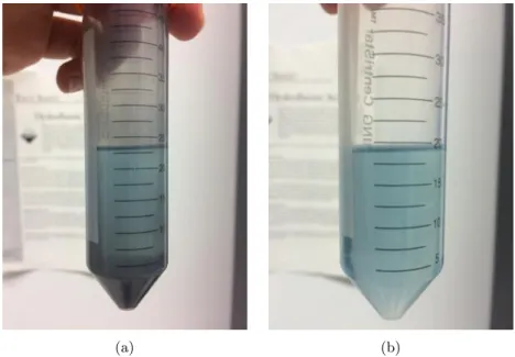
3.3 BBNP sample before centrifugation (a) and its dispersion after centrifugation (b) where is possible to see many flakes were too big to be mono-layers and therefore settled at the bottom after centrifugation.. . . 36
3.4 BBNP sample absorption spectrum with the orange lines showing the obtained bands and the green ones showing the wavelengths at which they were expected. 37 3.5 SEM images for the BBNP sample with (a) an overview of the sample, (b) an image of one of the bigger flakes and (c) shows signs of deformation on the flakes. 38 3.6 BBNP thickness measurement through SEM showing a thickness of 673 nm for this flake. . . 38
3.7 BBP sample before centrifugation (a) and its dispersion after centrifugation (b) showing a substantial decrease in the concentration of the dispersion after centrifugation. . . 39
3.8 BBP sample absorption spectrum with the expected wavelengths in green and the obtained ones in orange. . . 40
3.9 SEM images for the BBP sample with (a) an overview of the sample and (b) an image of a single flake. . . 41
3.10 BBP thickness measurement through SEM showing a thickness of 224 nm for this flake. . . 41
3.11 TEM images for the BBP sample with (a) an overview of two layers on top of each other, (b) observed Moiré lines, (c) image showing a flake with various thicknesses and (d) an observation of the x-ray diffraction pattern showing the crystalline structure of the sample. . . 42
3.12 Average Raman Intensity for BBP with the lines in orange and green showing the obtained shifts and the expected ones respectively. . . 43
3.14 BHNP sample after centrifugation (a) and its dispersion (b) showing a slight decrease in the concentration after removing the heavier flakes through centrifu-gation. . . 44
3.15 BHNP sample absorption spectrum with the expected wavelengths and the obtained ones in green and orange respectively. . . 45
3.16 SEM images for the BHNP sample with (a) an overview of the sample and (b) and (c) images of the obtained flakes. . . 46
3.17 BHNP thickness measurement through SEM showing a thickness of 351 nm for this particular flake. . . 46
3.18 Average Raman Intensity for BHNP with the lines in orange and green showing the obtained shifts and the expected ones respectively. . . 47
3.19 Raman intensities for BHNP between 402 and 405 cm−1 (a) and between 407
and 410 cm−1 (b), with (a) showing a higher predominance of the Raman Shift
respective to the cleaved layers. . . 47
3.20 BHP sample before centrifugation (a) and its dispersion after centrifugation (b), showing that most obtained particles were very large to remain in the dispersion after centrifugation. . . 48
3.21 BHP sample absorption spectrum with the expected wavelengths for MoS2
mono-layers in green and the obtained ones in orange. . . 49
3.22 SEM images for the BHP sample with (a) and (b) overviews of the obtained sample with some visible surface from the PVDF membrane and (c) showing a large defect on the observed flake. . . 50
3.23 BHP thickness measurement through SEM with 300 nm in thickness for this particular flake. . . 50
3.24 C_NP sample before centrifugation (a) and its dispersion after centrifugation (b) with a very clear colour. . . 51
3.25 C_NP sample absorption spectrum with the obtained wavelengths overlapped by the orange line and the expected ones by the green one. . . 52
3.26 SEM images for the C_NP sample with (a) and (b) overviews of the sample and (c) a detailed image from the surface of one flake. . . 53
3.27 C_NP thickness measurement through SEM indicating a thickness of almost 600 nm for this flake. . . 53
3.28 MBP sample before centrifugation (a) and its almost clear dispersion after centrifugation (b). . . 54
3.29 MBP sample absorption spectrum with the expected wavelengths in green and the obtained ones in orange. . . 55
3.30 SEM images for the MBP sample with an overview of the sample (a), (b) an image of a flake from this sample and (c) shows a flake folded on top of one of the peaks from the surface of the PVDF membrane. . . 56
3.31 Dispersions used for both the BBNP 20min and BBP 20min. . . 57
3.32 BBNP 20min sample absorption spectra with the expected and obtained
wave-lengths in green and orange respectively. . . 58
3.33 Overview of three MoS2 flakes from the BBNP 20min sample obtained through the SEM, with (b) showing the flakes on the border of a hole on the carbon grid and (c) an unknown deformity.. . . 59
3.34 BBNP 20min thickness measurement through SEM. . . 59
3.35 BBP 20min sample absorption spectra with the green line indicating the ex-pected wavelengths and the orange line the obtained ones. . . 60
3.36 SEM images for the BBP 20min sample with two flakes on (a) and (b) and a folded flake on (c). . . 61
3.37 BBP 20min thickness measurement through SEM showing a thickness of 342 nm for the observed flake. . . 62
3.38 Optical Microscope images at normal light from a bag without pits after expo-sition to intense cavitation for 0min (a), 20min (b) and 30min (c) showing no signs of damage from cavitation. . . 63
3.39 Optical Microscope images at normal light (left) and polarised light (right) from a bag with pits after exposition to intense cavitation for 0min (a) and (b), 2min (c) and (d), 10min (e) and (f) and 30min (g) and (h) showing no signs of damage caused by cavitation. . . 64
3.40 Optical Microscope images at normal light from a bag without pits after expo-sition to intense cavitation for 5min from an ultrasonic horn placed in contact with it. . . 65
4.1 Compilation of the UV-vis Absorption spectrum from all samples with the green lines pointing the wavelengths for the MoS2 mono-layers bands. . . 68
4.2 PVDF membranes with the obtained MoS2. . . 69
4.3 Average Raman Intensity for samples BHNP and BBP with the green lines indicating the Raman Shift for bulk MoS2, clearly showing the downshift in intensity for the obtained samples due to the presence of mono-sheats. . . 70
4.4 Example of MoS2 spill from the bag into the bath. . . 73
A.1 . . . 81
A.2 . . . 82
A.3 . . . 82
A.4 . . . 83
A.5 . . . 83
A.6 . . . 84
A.7 . . . 84
A.8 . . . 85
A.9 . . . 85
A.11 . . . 86
A.12 Normalised absorption spectra for a maximum absorption intensity of 0,352 at the wavelength of 699 nm. . . 87
A.13 . . . 88
A.14 . . . 88
A.15 . . . 89
A.16 . . . 89
A.17 . . . 90
A.18 . . . 90
A.19 . . . 91
A.20 . . . 91
A.21 . . . 92
A.22 . . . 92
A.23 . . . 93
A.24 . . . 93
A.25 . . . 94
A.26 . . . 94
A.27 . . . 95
A.28 . . . 95
A.29 Normalised absorption spectra for a maximum absorption intensity of 0,969 at the wavelength of 758 nm. . . 96
A.30 . . . 97
A.31 . . . 97
A.32 . . . 98
A.33 . . . 98
A.34 . . . 99
A.35 . . . 99
A.36 . . . 100
A.37 . . . 100
A.38 . . . 101
A.39 . . . 101
A.40 . . . 102
A.41 . . . 102
A.42 . . . 103
A.43 . . . 103
A.44 . . . 104
A.45 . . . 104
A.46 . . . 105
A.47 . . . 105
A.48 . . . 106
A.49 . . . 106
A.50 . . . 107
A.51 . . . 107
A.52 . . . 108
A.53 . . . 108
A.54 . . . 109
A.55 . . . 109
A.56 . . . 110
A.57 Normalised absorption spectra for a maximum absorption intensity of 0,278 at the wavelength of 686 nm. . . 111
A.58 . . . 112
A.59 . . . 112
A.60 . . . 113
A.61 . . . 113
A.62 . . . 114
A.63 . . . 114
A.64 . . . 115
A.65 . . . 115
A.66 . . . 116
A.67 . . . 116
A.68 Normalised absorption spectra for a maximum absorption intensity of 0,221 at various wavelengths between 714 nm and 724 nm.. . . 117
A.69 . . . 118
A.70 . . . 118
A.71 . . . 119
A.72 . . . 119
A.73 . . . 120
A.74 . . . 120
A.75 . . . 121
A.76 . . . 121
A.77 . . . 122
A.78 . . . 122
A.79 Normalised absorption spectra for a maximum absorption intensity of 0,129 at the wavelength of 680 nm. . . 123
A.80 . . . 124
A.81 . . . 124
A.82 . . . 125
A.83 . . . 125
A.84 . . . 126
A.85 . . . 126
A.86 . . . 127
A.88 . . . 128
A.89 . . . 128
A.90 Normalised absorption spectra for a maximum absorption intensity of 0,210 at the wavelength of 758 nm. . . 129
A.91 . . . 130
A.92 . . . 130
A.93 . . . 131
A.94 . . . 131
A.95 . . . 132
A.96 . . . 132
A.97 Normalised absorption spectra for a maximum absorption intensity of 0,131 at the wavelength of 895 nm. . . 133
A.98 . . . 134
A.99 . . . 134
A.100. . . 135
A.101. . . 135
A.102. . . 136
A.103. . . 136
A.104. . . 137
A.105. . . 137
A.106. . . 138
A.107. . . 138
A.108. . . 139
A.109. . . 139
A.110. . . 140
A.111. . . 140
A.112. . . 141
A.113. . . 141
A.114. . . 142
A.115. . . 142
A.116. . . 143
A.117. . . 144
A.118. . . 144
A.119. . . 145
A.120. . . 145
A.121Normalised absorption spectrum showing the maximum absorption intensity was not reached at the wavelengths close to the bands respective to the MoS2
nano-sheets. . . 146
A.122. . . 147
A.123. . . 147
A.124. . . 148
A.125. . . 148
A.126. . . 149
A.127. . . 149
2.1 Samples Description. . . 16
3.1 Buffer solution preparation. . . 54
4.1 MoS2 masses obtained after vacuum filtration through the PVDF membranes. 69
C h a p t e
1
I n t ro d u c t i o n
1.1
Sonochemistry
Acoustic cavitation is the formation and collapse of vapour cavities on a liquid volume from an external negative pressure [1] induced by a high-intensity ultrasound to a system. This ultrasound has various effects on the system, from chemical to physical. The chemical effects it can induce in a system can fall in three categories: homogeneous sonochemistry of liquids, heterogeneous sonochemistry of liquid-liquid or liquid-solid and sonocatalysis [2]. The physical effects involve enhanced mass transport, emulsification, bulk thermal heating and many other effects on solids such as exfoliation [3].
Despite being called sonochemistry, the effects from inducing a high-intensity ultrasound be-tween 20 kHz and 10 MHz [4] to a system are not a direct consequence from the ultrasound’s acoustic waves, since their dimension is much larger than the molecules’ dimensions [5]. Instead these effects arise from the cavitation generated from the ultrasound. It is possible to distinguish two types of cavitation, stable and transient. The first happens when the conditions allow for the bubbles to remain for extended periods of time without collapsing while sonication is applied. These bubbles oscillate radially around an equilibrium size persisting for many acoustic cycles. Whereas in transient cavitation the bubbles will persist only for one or two acoustic cycles. They grow to a size two or three times their original size during the negative acoustic pressures, when there is a rarefaction of the pressure on the solution, and collapse violently after a single compression half-cycle [6]. This later type of cavitation can be divided in three stages: nucleation, growth and collapse. Nucleation happens for the formation of the bubble. The sinusoidal wave that forms a sound is a mean through which energy is transported and it can be characterised by pitch, intensity and frequency, with the intensity, I, being given by equation 1.1, wherePA is the maximum
amplitude of the acoustic pressure, ρo the average density of the medium and V the sound
velocity [7].
I=PA2/2ρoV
(1.1)
The intensity differences in the sinusoidal wave create zones of rarefaction and compression in the pressure verified on the medium through which it propagates [8]. The differences in pressure from the acoustic longitudinal wave can be described as the movement of a spring and the differences it generates in the pressure of a liquid throughout space and time can be described by equation 1.2[6], whereP(t) is the total external pressure,P0 is the static
pressure and ω is the angular frequency of the acoustic wave.
P(t)=P0+PAsin(ωt)
(1.2)
This compression and expansion leads the liquid medium to a condition where its normal average pressure is exceeded and as a result, the distance between the molecules exceeds the critical molecular distance to hold the liquid intact and inevitably the liquid ruptures and generates bubbles of various sizes [7]. For distilled water at 22◦C the difference in
pressure needed to generate cavitation can vary from -0,1 MPa to -20 MPa if is saturated with air or degassed respectively [9]. In transient cavitation the bubbles must grow in size before collapsing. Just like a spring, the bubble gas-liquid interface will oscillate with the differences in pressure and the bubble will grow before collapsing. On the other hand, in stable cavitation, the bubble will shrink during the compressional phase of the sinusoidal wave and diffuse gas out into the medium. During the rarefaction cycle, it will expand due to the gas diffusions that happen, this time into the bubble. This process, shown in Figure 1.1, is called rectified diffusion and allows for the longer lifespan of the bubble when compared to transient cavitation [6]. Eventually, after some time, collapse occurs due to the pressure inside the bubble no longer being in equilibrium with the pressure verified in the medium. During their collapse are generated conditions with temperatures as high as 5000◦C, heating and cooling rates of 1010 K/s, and pressures close to 1000
Figure 1.1: Schematic representation for the growth and collapse of stable cavitation bubbles during the rectified diffusion process [11].
Tf=T0(Rm/Rf)3(γ−1)
(1.3)
Being Tf the final temperature of the gas within the bubble, T0 the liquid temperature,
Rm the maximum bubble radius,Rf the final bubble radius andγ the ratio of specific heat
for the liquid. Thus, the diffuse energy from sonication is concentrated in the bubbles and later released through these high temperatures and pressures [3]. The places where these conditions are verified are called hot spots. Here, the chemical and mechanical consequences of sonication are verified with the formation of radical species that interact with the species of the medium, sonochemiluminescence, from the recombination of the radical species [6], the occurrence of shock waves and other shear forces, which contribute to the mixing and particle fragmentation of the solids present in the medium [12], and sonoluminescence, when there is light emission from the bubble collapse [13].
Figure 1.2: Schematic representation of the various chemical and physical effects from cavitation [2].
Three regions of sonochemistry have been identified for analysis of the behaviour of the bubble: bubble interior, bubble gas-liquid interface and liquid bulk [12]. The chemical effects derived from cavitation such as radical and excited species formation from molecular sonolysis, polymer rupture and changes in ligand-metal coordination mainly occur in the bubble interior or at the bubble interface. Later, these new species diffuse to the liquid bulk. The mechanical effects, on the other hand, are a result from the shockwaves, liquid jets and shear forces generated by the bubble collapse and therefore occur on the bulk liquid. When these effects act within the hot spot domain it is called primary sonochemistry and secondary sonochemistry when they act outside as depicted in Figure 1.3[7].
Figure 1.3: Schematic representation of primary and secondary effects of cavitation [7].
When it comes to radical generation the species generated in an aqueous solution are well known to be H•and OH• radicals [5,14]. The generation of radicals is highly dependable on
the conditions verified on the medium upon cavitation. These radicals besides interacting with the materials in solution, will recombine between themselves generating new species and sonochemiluminescence, from emitting light when interacting with other species in the solution outside the bubble [6,13]. For the aqueous solutions it is known that cavitation generates H2 and H2O2 [5].
Cavitation has different effects when it occurs close to a solid surface instead of inside a pure liquid. In liquid-solid sonication, the crevices of the solid play an important role in increasing the effects of sonication. These small crevices store air, and the interface between the air and the liquid that covers the surface of the solid, oscillates with the ultrasound to a point where it may break and generate more bubbles, maximising the sonication effects by increasing the number of bubbles in the medium. Also, near a solid surface the bubble collapse is non-spherical, like in Figure 1.4, creating a shockwave that damages the surface and may break up brittle materials through a high-speed liquid microjet, which can reach velocities as high as hundreds of meters per second [10]. These distortions on the bubble collapse are dependable on the surface size which must be several times larger than the resonance bubble size. Thus, for ultrasonic frequencies of approximately 20 kHz, there is no damage from microjet formation on solid particles smaller than 200 µm. Ultrasonic
cleaning is possible thanks to the erosion caused by these interactions between the bubbles and other solids in solution [3].
Figure 1.4: Formation of a liquid microjet near an extended surface [3].
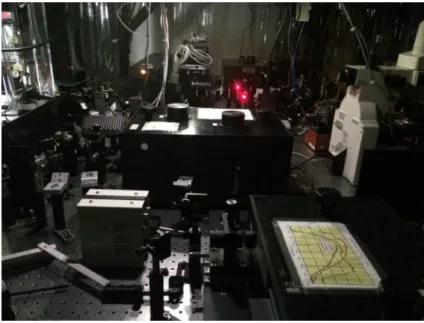
Currently there is a wide variety of sonochemical apparatus being the most common ul-trasonic cleaning baths, direct ulul-trasonic immersion horns and flow reactors. Cleaning baths are very useful for liquid-solid reactions despite having low intensities [10]. These apparatus have various transducers placed horizontally beneath the bath which induce the ultrasound on a liquid medium where the sample is placed. The ultrasonic horn, usually induces a higher intensity ultrasound on the solution through a titanium horn driven by a piezoelectric transducer into the sample, usually stored in a glass flask. These equipments operate at frequencies around the 40 kHz with the ultrasonic horns reaching the 20 kHz. Nonetheless, there are apparatus available for many other intensities [5].
(a)
(b)
Figure 1.5: Schematic Representation of the Ultrasonic Bath from Figure 2.4(a) and Horn from Figure 2.5(b), both applying ultrasound and generating bubbles.
control the frequency, intensity, pulse conditions, type of exposure field and total exposure time. As frequency increases, Rm will decrease resulting in less time for nucleation and
growth. Higher intensities result in bubbles of bigger dimensions and consequently higher temperatures. When it comes to the conditions of the liquid it is important to know all the properties of the liquid and if it is in the proper conditions for use in the experiment, since it will highly influence the radical generation. Finally, like in any other experiment the method of observation must be similar in every experiment. All these parameters must be carefully controlled since cavitation is a very difficult phenomena to quantify [6].
1.2
MoS
2Exfoliation
Due to the mechanical and chemical phenomena sonication generates, it can be used for a very particular and interesting process in nano-materials synthesis: exfoliation.
Currently, the research made on graphene, a two-dimensional network of sp2 carbon atoms, has placed it as the flagship material for future technology [7]. It is still being researched to this day a process adaptable to large-scale synthesis of few-layer graphene and other materials called transition metal dichalcogenides, TMDCs. These materials have very interesting properties when used in a single-layer disposition for various applications like energy storage, catalysis, solar cells, sensing and electronic devices. These substances are a very large family of layered materials with crystal structures covalently bonded in X-M-X layers that interact through van der Walls forces, being the M a metal atom such as Mo, W, Ti, Zr, Hf, Ta, Re, Co, Ni, Ir, Pt, V, Nb, Tc, Rh or Pd, and X a chalcogen like S, Se or Te, and therefore due to these various combinations, these materials can either be semiconductors, metallic or superconducting [17]. Each single-layer of a TMDC is a layer of a metal sandwiched between two layers of chalcogens. One of the most promising TMDCs is MoS2. Unlike graphite, molybdenum is a very common element and as a single-layer, MoS2, is a p-type semiconductor, or a metal depending on its metallic phase [18], that transits from the indirect bandgap it has in the bulk state of 1,2 eV to a a direct bandgap of 1,8 eV [19]. This property is very interesting since it largely compensates the weakness of gapless graphene, making it very useful for the next generation in switching and opto-electronics devices. A MoS2 mono-layer has a thickness of approximately 0.65nm [20]. In addition to the many applications of MoS2 as a three-dimensional material, its mono-layers can also be used for memory devices, photodetectors, photovoltaic devices, field effect transistors [17] and as an hydrogen evolution catalyst [21].
Figure 1.6: Chemical structure of two mono-layers of MoS2 (a), the two metallic phases from MoS2 as a mono-layer (b) and the two typical Raman active phonon nodes from this material [17].
In order to explore the interesting properties of these materials exfoliation is a mandatory step on their transition from a three-dimensional material to a two-dimensional one. To do so, many methods similarly used for the exfoliation of graphite into graphene may be implemented. These methods are either chemical, micromechanical, surfactant assisted liquid phase exfoliation or growth via chemical vapour deposition [22]. They can have a bottom-up approach or a top-down one [21]. Micromechanical cleavage techniques, such as the scotch tape method, rely on shear forces to overcome the weak forces that connect the various mono-layers and produce single-layered MoS2 with very high structural quality but lacks the scalability for practical applications. The more common chemical cleavage relies on lithium intercalation between the single-layers of the TMDC overcoming the weak van der Walls forces [23, 24] as in Figure 1.7. However, despite being a scalable process the chemical cleavage of MoS2 leads to a phase transition of the material to a metallic 1T-MoS2 from the original semiconducting 2H-MoS2 phase, needing further thermal treatments in order for the MoS2 to regain its original phase. Currently, research is being made on new
supercritical CO2 for the exfoliation of MoS2 mono-layers has been studied [26]. Thanks to the wide range of applications and properties of these material, new exfoliation methods are constantly being designed and tested but the lack of a simple and properly effective technique to exfoliate high-quality and defect free MoS2 has hampered important studies and practical applications of this material [21].
Figure 1.7: Representation of Li ions intercalation to later exfoliate MoS2 through water sonication [23].
1.3
Novel exfoliation process
With the enormous difficulties in finding a straightforward and simple technique to exfoliate and synthethise nanomaterials, it is worth attempting to explore the capabilities of the BuBclean Cavitation Intensifying Bags, CIBs orBuBble Bag - Figure1.8.
(a) (b)
Figure 1.8: BuBclean Cavitation Intensifying Bag [27] (a) and a schematic representation of the same bag showing the pits as a mean to intensify bubble nucleation [28] (b).
rely on small fractures and crevices on its surface to store small bubbles of air to generate cavitation, this setup already possesses the much needed crevices as the pits. The existence of pits not only enhances the intensity of the generated cavitation but also increases the reproducibility of the work done with the bags [16], a critical factor when working with sonochemistry.
C h a p t e
2
T e c h n i q u e s a n d M at e r i a l s
2.1
Materials
This section describes the materials used in the experimental work made throughout this work, from reactants, solvents and other substances used.
2.1.1 Molybdenum(IV) Disulfide
In this work Molybdenum(IV) Disulfide, MoS2, - fromAldrich Chemical - was the compound chosen to prove the exfoliation capabilities of the BuBclean bags. This compound is a very thin dark powder with a molecular weight of 160.07 g.mol−1 and a density of 5.06 g.mL−1
at 20◦C. It is sold in the form of powder under the CAS number 1317-33-5.
Figure 2.1: MoS2 chemical structure.
2.1.2 Isopropanol
Isopropanol (C3H8O) was used as the main solvent in this experiment. Acquired from Atlas Assink Chemie, it has a molecular weight of 60,10 g.mol−1, a density of 0,786 g.mL−1
at 20◦C and is a colourless liquid. It must remain away from fire due to its inflammable
nature. It is identified under the CAS number 67-63-0.
2.1.3 Buffer Reactants
For this work a few reactants were used to adapt samples for certain observations. These reactants were used as radical trappers and to prepare a buffer solution. These were:
• Terephthalic Acid
Terephthalic Acid was used on this work as a radical scavenger. It has a molecular weight of 166.13 g.mol−1, has a density of 1,522 g.mL−1 at 20◦C and resembles a
white powder. It was supplied byAldrich Chemicaland is sold under the CAS number 100-21-0.
Figure 2.2: Terephthalic Acid chemical structure.
• Sodium Hydroxide
Sodium Hydroxide (NaOH), was one of the compounds used in the preparation of the solution for the radical trapping. This compound is a strong base and was supplied from Aldrich Chemical. It has a molecular weight of 39,9971 g.mol−1, a density of
2,13 g.mL−1 at 20◦C and has the appearance of small white crystals. It is identified
by the CAS number 1310-73-2.
• Monopotassium Phosphate
Supplied by Riedel-de Häen, Monopotassium Phosphate (KH2PO4) or Potassium Dihydrogen Phosphate was one of the two compounds used in the preparation of a buffer solution. It has a molecular weight of 136,086 g.mol −1, has a density of
2,338 g.mL−1 at 20◦C and is a thin deliquescent white powder. It is identified by the
CAS number 7778-77-0.
• Disodium Phosphate
Disodium Phosphate (Na2HPO4) or Sodium Hydrogen Phosphate was acquired to Riedel-de Häen. It is a white powder, with a molecular weight of 141,96 g.mol−1 and
a density of 1,7 g.mL−1 at 20◦C. It is identified by the CAS number 7558-79-4.
2.1.4 Azobisisobutyronitrile
Azobisisobutyronitrile (AIBN) is a compound commonly used in polymer science as an initiator to generate radicals which will begin the polymerisation process. It was used in order to generate radicals without resorting to cavitation and this way avoid any mechanical effects from it.
The used AIBN was from Aldrich Chemical. It has a molecular weight of 164,21 g.mol−1,
a density of 1,1 g.mL−1 at 20◦C and is identified under the CAS number 78-67-1. It must
be stored on a fridge at a temperature between 2-8◦C, otherwise it will start to decay.
Figure 2.3: Formation of radicals from AIBN [30].
2.1.5 Cavitation Intensifying Bags
The Cavitation Intensifying Bags used were produced by the company BuBclean. The bags used were made of polyethylene or polypropylene, with a wall thickness of 5µm and
dimensions of 100x150 mm. These bags are made industrially through the pressing of a cast with pins on the inside side of the bag before it being folded. It was both used bags with pits and without pits.
2.2
Techniques
2.2.1 Solution Preparation
2.2.1.1 MoS2 Exfoliation
This study followed an adaptation of the procedure used by Mandal [31] for the function-alization of MoS2 flakes and by Coleman [32].
M o S2 E x f o l i at i o n w i t h t h e BuBclean b a g s i n t w o d i f f e r e n t
s e t u p s
For the experimental setup of this experiment were prepared the samples describe on table
2.1 in order to analyse the differences in the product obtained when comparing different ultrasonic sources and different bags. The solution inside the bag is a mixture of IPA and MoS2 with a concentration of 20 mg.ml−1. This mixture is called Basic because it does not
contain radical scavengers nor an initiator to produce radicals like in other two solutions prepared to understand the exfoliation process as described later.
Sample Solution Ultrasonic Type of Bag Time
Equipment of Sonication
BBP Basic Ultrasonic Bath Bag with Pits 4,5 hours BBNP Basic Ultrasonic Bath Bag without Pits 4,5 hours BHP Basic Ultrasonic Horn Bag with Pits 4,5 hours BHNP Basic Ultrasonic Horn Bag without Pits 4,5 hours BBNP 20 mins Basic Ultrasonic Bath Bag without Pits 20 mins BBP 20 mins Basic Ultrasonic Bath Bag with Pits 20 mins
Table 2.1: Samples Description.
Inside the bags used for the Ultrasonic Bath (VWR USC200TH), were placed 50 ml of IPA whereas for the bags placed inside the Ultrasonic Horn (Bandelin Sonoplus mini20) were only placed 25 ml. This is because the bags for the horn were modified into a slightly smaller size due to the fact that the biggest probe (MS 2.5) available for the horn is used for 25 ml samples. Most samples were exposed to ultrasound for 4,5 h [31]. Later, two samples were exposed to ultrasound solely for 20 mins to observe how the difference in time and energy would affect the final result.
hands in the liquid exposed to ultrasound since it may generate air bubbles in the blood stream.
Figure 2.4: VWR USC200TH Ultrasonic Bath with a capacity of 1,8 L and a frequency of 45 kHz. This equipment is 17,5 cm wide, 16,5 cm deep and 22,5 cm height.
Figure 2.5: Bandelin Sonoplus mini20 Ultrasonic Horn with the MS 2.5 probe applies a frequency of 50/60 Hz and has 0,5 cm in diameter at the tip and 16 cm in height.
After sonication these samples were taken for centrifugation for 1 h at 1500 rpm at a Heraeus Labofuge 400 like the one shown in Figure 2.6. This way the heavier parts of the solution
would deposit at the bottom of the flask. Later, on top of this residue is a dispersion of IPA and the lighter parts of MoS2. A third of this dispersion was retrieved and taken for analysis with the UV-Spectrophotometer. The dispersion left from the absorption measurements was then vacuum filtrated to retrieve the MoS2 that stands on the dispersion. For this a PVDF membrane with 0,1µm pore size fromMerk Millipore was used. By measuring the volume before the filtration and the mass that is deposited on the membrane is possible to compare the various results. The volume is measured before the filtration because IPA easily evaporates through the hose that induces the vacuum. For the rest of the tests done, small pieces of the membrane were cut and used for each method after 24 h in the oven at 80◦C to evaporate any remaining solvent. A diaphragm vacuum pump from vacuubrand
type MZ 2C with a pump flow of 1,7 m3/h was used.
E x f o l i at i o n a s a r e s u lt o f C h e m i c a l o r P h y s i c a l e f f e c t s
To observe if the exfoliation process occurs due to chemical or mechanical effects from cavitation a setup was devised where each of these effects would be removed from the experiment.
To remove any chemical effects, the solution MBP was prepared by adding to the solution of IPA and MoS2, 5 mL of a solution [14] that acts as a radical scavenger. This way as radicals are generated, they are trapped by the scavenger solution and any interactions that may happen between the MoS2 and the radicals is minimized. The scavenger solution used was prepared by mixing 0.0834 g (2 mmol.L−1) of terephthalic acid, 0.0529 g of NaOH
(5 mmol.L−1), and phosphate buffer with a pH of 7.4, prepared from 0.1480 g of KH
2PO4 (4.4 mmol.L−1) and 0.2453 g of Na2HPO4 (7 mmol.L−1). The solution was then placed
inside a bag with pits, to maximise the mechanical effects, and on the ultrasonic bath. On another experiment, the mechanical or physical effects were removed by not applying ultrasound to the solution. Instead, approximately 1 mg of AIBN was introduced to a basic solution of MoS2and IPA, which was heated to a temperature of 60◦C. A temperature high
enough for AIBN to generate radical species but still too low for IPA to boil. This solution was prepared inside a beaker and had a mixer at low speeds to avoid much turbulence, which would otherwise cause itself physical effects on the MoS2 particles. The beaker was covered with Parafilm MR to avoid losing sample from evaporation. This sample was called C_NP.
The following diagrams in Figures 2.7, 2.8, 2.9 and 2.10 show the procedure used for all the samples and all the analysis done to each:
Bulk SEM
Figure 2.7: Experimental procedure used for the analysis of the Bulk sample.
BBNP, BBP, MBP Sonication4,5 h Bath
BHNP, BHP Sonication4,5 h
Horn Centrifugation 1 h 1500 rpm Absorption Spectrum of the Dispersion Vacuum
Filtration PVDF membrane Oven
24 h 80◦C
MBP TEM Fluorescence Spectrum SEM BHNP, BHP, BBNP, BBP, MBP Raman BBP, BHNP
Figure 2.8: Experimental procedure used for the analysis of the BBNP, BBP, BHNP, BHP and MBP samples.
C_NP
Low Speed Mixing &Heating
60◦C
Centrifugation 1 h 1500 rpm
Absorption Spectrum of the Dispersion Vacuum
Filtration PVDF membrane SEM
BBNP 20min, BBP 20min
Centrifugation 1 h 1500 rpm
Sonication 20 min
Bath Dispersion
Absorption Spectrum SEM
Figure 2.10: Experimental procedure used for the analysis of the BBNP 20min and BBP 20min samples.
2.2.1.2 Resistance of the BuBclean bags to Cavitation
On this experiment are evaluated the effects from cavitation on the bags. As known, cavi-tation generates very intense phenomena that can have effects on the physical and chemical stability of the polypropylene of which the bags are made.
A small piece of aBuBclean bag with approximately the size of a cover slip was cut from the top side of the bag, where there are no pits. This bag sample was then attached to a cover slip with the help of two smaller pieces of another cover slip and scotch tape, as shown in Figure 2.11.
Figure 2.11: Sample preparation.
The sample was placed inside a small glass reservoir with 200 mL ofMili-Q water and an ultrasonic horn, being held by a grip, was placed 5 mm above the sample and turned on for 2, 5 and 10 minutes. The sample was divided in three parts to allow three measurements with just one sample. These samples are then observed through the SEM to analyse any erosion that may take place.
In another attempt to observe changes on the bag after sonication, the bag was placed on the same glass reservoir as before and in the same conditions, but was exposed to ultrasound and then observed through the optical microscope until there were signs of erosion on its surface. Polarised lenses were used to help identifying small signs of erosion. The ultrasonic horn was placed 5 mm above the sample.
This experiment is a continuation of the ongoing resarch by Rivas on the erosion from acoustic cavitation on silicon surfaces [1].
2.2.2 Characterisation Methods
2.2.2.1 Spectrometry
Absorption Spectra
This method was used to qualitatively and quantitatively observe if the compounds on the dispersion are the ones which are intended to be produced and compare between samples their respective yield. This equipment uses a light beam of an identified wavelength to analyse what wavelengths are absorbed by the sample. An initial blank measurement is made to establish a zero absorption spectrum. Afterwards, a light beam is directed towards the sample and then captured through a detector. This detector measures the difference in the intensity of the light beam after passing the sample. This intensity is then subtracted to the intensity from the blank solution generating the absorption spectrum. During every measurement two cuvettes stand inside the spectrophotometer. One just with solvent and the other with the sample from the solution. This way the absorption from the solvent is not taken into account by the detector.
The Beer-Lambert Law makes it possible to relate the absorption from a sample with its concentration through equation 2.1.
A=ε×l×c
(2.1)
Being Athe absorption intensity, lthe cuvette’s length, c the sample’s concentration and εthe extinction coefficient. Since the sample’s concentration is unknown it is necessary to
determine the extinction coefficient value. For that, a series of five dilutions are made and the respective spectra peak are measured. After measuring the solution volume and the mass obtained through the filtration it is finally possible to determine the concentration from each of the five dilutions and relate it with the respective absorption bands. This relation returns a linear equation whose slope is the extinction coefficient.
Figure 2.13: Perkin Elmer Lambda 850 UV-Spectrophotometer.
Raman Spectroscopy
Raman Spectroscopy is a method used to identify species through their vibrational, rota-tional and low-frequency modes. The monochromatic light from a laser is used to excite the rotational modes of the species present in the sample. Leading the phonons on the laser to shift in energy, which allows for the identification of the species present in the sample. Usually the laser is either on the visible spectra, close to the infrared, or in the infrared wavelength. The resulting data from this test is a simulated image from the area of the sample where the laser ran. This image indicates the Raman intensity for every point of that area and can be transformed into a graphic that indicates the average Raman intensity for the sample. From the generated graphic is possible to analyse the sample both quantitatively by analysing the peak intensity, and qualitatively by observing the obtained Raman shifts for each peak.
Ideally the samples for observation on this equipment are placed on top of a calcium fluo-ride holder to reduce the fluorescence and for the sample to have a flat surface. A silicon wafer can also be used as a holder. On this experiment the holder where the sample was placed was the membrane where it had been filtrated. The membrane is far from an ideal holder due to its high fluorescence and rugosity. Intense fluorescence results in high Raman intensities and the variable rugosity of a sample makes impossible for an even measurement since the laser propagates for a small distance into the surface of the sample and in these conditions sometimes the measurements may contain some air due to a lower thickness of the sample.
For this work was used the Raman apparatus from the Medical Cell BioPhysics research group from the University of Twente seen in Figure 2.14. It applied a laser beam with a power output of 350 µW, a frequency of 50 kHz for 50 ms over a surface with 50x50 µm.
Figure 2.14: Raman Spectrophotometer at the Medical Cell BioPhysics research group.
Fluorescence
To measure the amount of radicals captured by the radical scavenger in the analysis made to either it is the mechanical effects or the physical effects that generate the exfoliation process, it was necessary to evaluate the concentration of the therephthalic acid present in the solution.
On this method, a light beam of know wavelength is directed to the sample. On the case of the therephthalic acid it is know that when a wavelength of 315 nm is used, its electrons reach an excited singlet state and when they return to their electronic ground state, emit photons with a wavelength of 425 nm. The fluorescence spectrophotometer then detects this emission and generates a graphic where is possible to observe the emission intensity of the photons emitted by the sample. Expectably, in the picked wavelength interval there should only be a peak at the previously known emission wavelength. It is also possible to make the opposite analysis by analysing the excitation of the sample instead of the emission.
For this work a Perkin Elmer fluorescence spectrophotometer was used - Figure 2.15. The sample is a small volume of the obtained dissolution which is placed in a cuvette. Fluo-rescence measurements, unlike absorption, are made in a 90◦ angle. This means that the
wavelength detected is measured in a plane that is 90◦ to the face of the cuvette where
Figure 2.15: Perkin Elmer fluorescence spectrophotometer.
fluorescence intensity detected is satisfactory. It is important to avoid exposing the sample to too much light because this may compromise the results obtained through this method. To determine the concentration of terephthalic acid on solution and then calculate the amount of radicals that were generated and trapped by the scavenger the same procedure used for absorption with the Beer-Lambert Law is used.
2.2.2.2 Microscopy
Scanning Electron Microscopy
The scanning electron microscope (SEM) is used for the observation of a samples’ topog-raphy and can also be used to determine its surface composition. This microscope is different from the more common microscopes since it relies on an electron beam and the particles emitted by the sample upon being hit by it to generate a two dimensional image and to determine which compounds are present on the surface. This procedure allows for resolutions as high as 25 Å, much higher than the resolutions obtained through common microscopes.
For this procedure a Zeiss Merlin SEM as seen in Figure 2.16 was used. This equipment, as any other SEM, is composed of two main parts: the electron column and the control console. The electron column is where the electron beam is generated and directed towards the sample which is also stored on this part of the SEM. This segment of the equipment is in vacuum during the observation and also contains electromagnetic deflectors to direct the beam towards the sample. To produce the electron beam a tungsten filament is heated to very high temperatures to generate free electrons. These electrons are accelerated through the column by a potential difference and pass through lenses which converge the beam through the focal point. For the samples observed in this work various potential differences
Figure 2.16: Zeiss Merlin Scanning Electron Microscope [34].
were used. When the beam reaches the sample chamber and hits the surface of the sample various particles are released due to the kinetic energy of the electrons. This kinetic energy leads to two different types of scattering interactions with the sample which translates into two different types of particles: secondary electrons, when there are inelastic scattering interactions, and backscattered electrons, for when the scattering interactions are elastic. Both are detected by a detector in the sample chamber and used to generate the SEM image, being the first important in analysing the topography and morphology of the sample and the latter in showing contrast between areas of different chemical composition. X-rays are occasionally emitted when an inner shell electron is removed from the sample and can be used to determine the sample’s chemical composition.
For this method a small piece of the membrane used for the filtration with sample was cut and placed on a metal holder for observation. For a second batch of samples, a drop of their dispersion was placed on top of a carbon grid for better images. To observe the ef-fects from cavitation on the bag, the entire sample was placed inside the equipment as it was.
Transmission Electron Microscopy
A transmission electron microscope is also made up of an electron column and a control panel. A Phillips CM300ST-FEG transmission electron microscope - Figure 2.17 - was used.
For this method, a part of the dilution obtained of the sample to be observed was not filtrated. Instead a small drop of it was placed on a carbon grid. This grid serves as a holder which is then placed in the electron column for the observations.
Figure 2.17: Philips CM300ST-FEG Transmission Electron Microscope 300 kV [35].
Optical Microscope
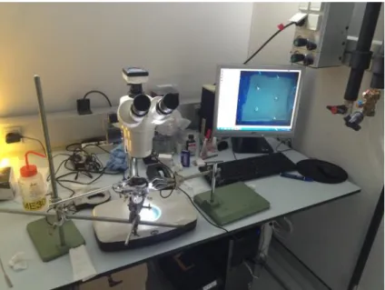
For the observation of the erosion effects from cavitation on the bags was used the Motic microscope seen in Figure2.18. This microscope had a camera (Moticam 1SP with 1.3 MP) that transmitted the captured image to a computer from where the obtained images were captured. To capture the images were used the programs Motic Live Imaging Module and Motic Images Plus 2.0 ML.
The polarised lenses from ThorLabs Inc. shown in Figure 2.19 were used to detect any initial signs of erosion before being observable through normal lenses. The lenses and sample were placed together with the microscope as can be seen from Figure 2.18. By placing these lenses in a cross planar angle as in Figure 2.20 is possible to observe the sample through a light that has only one orientation.
Figure 2.18: Motic microscope and the used setup for the observations.
Figure 2.20: The polarisers only allow for the observation of the light oriented in one direction.
C h a p t e
3
E x p e r i m e n ta l R e s u lt s
In this chapter will be presented and analysed the results from this work.
On this work was attempted the applicability of the CIBs for the exfoliation of MoS2 using two different types of sonication equipment. It was also studied on whether it is the physical or chemical effects from cavitation that induce the exfoliation of the bulk material by inhibiting interactions between the formed radicals and the MoS2 and not generating mechanical effects.
On another experiment, it was studied if the CIBs suffered significant damage from the cavitation effects on its surface.
All the images and other data obtained for the following samples can be viewed on the AppendixA.1. On this chapter is presented a selection of the more interesting data.
3.1
MoS
2Liquid-Phase Exfoliation in Cavitation
Intensifying Bags
For this experiment, were firstly measured the absorption spectra of the obtained MoS2 dispersions. With this first step was intended to determine if there were MoS2 mono-layers present in the solution. Afterwards were made the SEM and TEM observations. Later the qualitative analysis made with the absorption spectra were verified with another measurement, this time with the Raman Spectra.
Due to timing and technical factors not every sample went through all the measurements.
3.1.1 Bulk
S E M
As a reference for other SEM observations, a sample solely with bulk MoS2 was observed. This sample was not exposed to ultrasonic conditions - Figure2.7. Instead, it was observed as it was received from the manufacturer.
(a) (b)
(c) (d)
Figure 3.1: SEM images of Bulk MoS2 flakes.
Figure 3.2: Thickness measurement through SEM to a Bulk MoS2 flake.
As seen from Figure 3.2 measuring flake thickness from SEM is not an accurate pro-cedure. It can be used for reference but is dependent of the spacial orientation of the flake, as can be seen from the significant difference in thickness measured for the same flake in Figure 3.2, where two thicknesses of 802,1 nm and 558,4 nm were measured.
3.1.2 BBNP - Basic, Ultrasonic Bath, No Pits
Sample prepared with a concentration of 20 mg.ml−1 MoS2 in 50 mL of IPA. It was
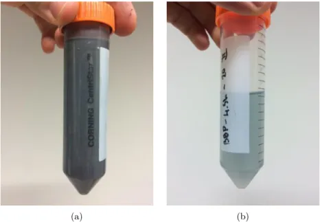
soni-cated in the ultrasonic bath for 4,5 h with tap water, inside a bag without pits - Figure2.8. The dispersion obtained after centrifugation showed there were some particles dispersed in the solvent indicating there were particles in solution light enough to not settle at the bottom of the centrifugation flask. The differences in the sample concentration can be observed in Figure 3.3 by the difference in colour before centrifugation and the obtained dispersion.
(a) (b)
Figure 3.3: BBNP sample before centrifugation (a) and its dispersion after centrifugation (b) where is possible to see many flakes were too big to be mono-layers and therefore settled
at the bottom after centrifugation.
A b s o r p t i o n S p e c t r a
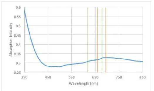
Figure 3.4: BBNP sample absorption spectrum with the orange lines showing the obtained bands and the green ones showing the wavelengths at which they were expected.
S E M
Images at different resolutions are shown in Figure 3.5from the morphology studies of this sample of MoS2.
This study showed that there were still very thick layers of MoS2 in this sample. Compared to the images of bulk MoS2 flakes, these flakes appear more eroded and regular on the edges. From the SEM observations was possible to determine that one of the flakes from this sample measured about 673 nm in thickness as seen in Figure 3.6.
(a) (b)
(c)
Figure 3.5: SEM images for the BBNP sample with (a) an overview of the sample, (b) an image of one of the bigger flakes and (c) shows signs of deformation on the flakes.
3.1.3 BBP - Basic, Ultrasonic Bath, Pits Sample prepared with a concentration of 20 mg.ml−1 MoS
2 in 50 mL of IPA. It was soni-cated in the ultrasonic bath for 4,5 h with tap water, inside a bag with pits - Figure 2.8. The dispersion obtained after centrifugation showed there were some particles dispersed in the solvent. The visual differences in the sample concentration can be observed in Figure 3.7by the difference in colour before centrifugation and the obtained dispersion.
(a) (b)
Figure 3.7: BBP sample before centrifugation (a) and its dispersion after centrifugation (b) showing a substantial decrease in the concentration of the dispersion after centrifugation.
A b s o r p t i o n S p e c t r a
The absorption spectra from the BBP sample showed the distinct bands of MoS2 mono-layers. However these bands appeared fused. The bands were considered at 655nm and 691nm - Figure 3.8. From these results was proven the existence of MoS2 mono-layers in the solution [32,36].
Figure 3.8: BBP sample absorption spectrum with the expected wavelengths in green and the obtained ones in orange.
S E M
In Figure 3.9are shown three images at different resolutions from the morphology studies of this sample of MoS2.
(a) (b)
Figure 3.9: SEM images for the BBP sample with (a) an overview of the sample and (b) an image of a single flake.
Figure 3.10: BBP thickness measurement through SEM showing a thickness of 224 nm for this flake.
T E M
A drop of the dispersion from this sample was used to generate the images in Figure 3.11, which show that flakes on the dispersion are very thin since it is possible to observe layers beneath the top layer. It is also possible to observe Moiré lines meaning the layers are not aligned on top of each other. Observations on the crystalline structure of the layers con-firmed that the observed crystalline structure on the obtained flakes matches the original 2H-MoS2 semiconducting phase of bulk MoS2.
R a m a n S p e c t r a
The Raman Spectra measurements for this sample were done with a power of 350µW for
50 ms, with a frequency of 50 kHz and through an area of 50x50 µm, which generated an
(a) (b)
(c) (d)
Figure 3.11: TEM images for the BBP sample with (a) an overview of two layers on top of each other, (b) observed Moiré lines, (c) image showing a flake with various thicknesses and (d) an observation of the x-ray diffraction pattern showing the crystalline structure of the sample.
image with 100x100 pixels.
From Figure 3.12 is possible to confirm the presence of MoS2 in the sample. From the slight downshift of the second peak, A1g, from 408 cm−1 to 403 cm−1 is possible to say
that there are micromechanically cleaved single layers of MoS2 present in the sample. The generated images in Figure 3.13 confirm this by showing that there are less areas with Raman intensity in the interval of 407 and 410 cm−1 than to 402 and 405 cm−1. These
Figure 3.12: Average Raman Intensity for BBP with the lines in orange and green showing the obtained shifts and the expected ones respectively.
(a) (b)
Figure 3.13: Raman intensities for BBP between 402 and 405 cm−1 (a) and between 407
and 410 cm−1 (b) showing that the areas with the Raman intensity for cleaved layers,
403 cm−1, is more predominant than the areas with the Raman intensity associated to
408 cm−1.
3.1.4 BHNP - Basic, Ultrasonic Horn, No Pits Sample prepared with a concentration of 20 mg.ml−1 MoS
2 in 25 mL of IPA. It was sonicated in the ultrasonic horn for 4,5h inside a bag without pits - Figure 2.8.
The dispersion obtained after centrifugation showed there were some particles dispersed in the solvent proving there were particles in solution light enough to not settle at the bottom of the centrifugation flask.
(a) (b)
Figure 3.14: BHNP sample after centrifugation (a) and its dispersion (b) showing a slight decrease in the concentration after removing the heavier flakes through centrifugation.
A b s o r p t i o n S p e c t r a
Figure 3.15: BHNP sample absorption spectrum with the expected wavelengths and the obtained ones in green and orange respectively.
S E M
In Figure 3.16are shown three images at different resolutions from the morphology studies of this sample of MoS2. From these pictures is observable that the obtained flakes are very different in sizes among them. There are large flakes dispersed on the surface as well as flakes of much smaller size. This can be explained due to the higher intensity of the ultrasonic horn on areas close to it and its weaker intensity on areas further away from it. This way the different intensities experienced by the bulk flakes on the various areas of the solution translates in flakes of various sizes.
This study also showed that there were still very thick layers of MoS2 in this sample. Through the SEM was possible to determine that one of the flakes from this sample measured about 351 nm in thickness as seen in Figure 3.17.
R a m a n S p e c t r a
The Raman Spectra measurements for this sample were done with a power of 350µW for
50 ms, with a frequency of 50 kHz and through an area of 50x50 µm, which generated an
image with 100x100 pixels.
Qualitatively was possible to confirm the presence of MoS2 on the surface of the PVDF membrane as seen in Figure 3.18. Due to the slight downshift of the second peak, A1g,
from 408 cm−1 to 403 cm−1 is possible to say that there are micromechanically cleaved
layers of MoS2 present in the sample. The generated images in Figure3.19confirm this by showing that there are less areas with Raman intensity in the interval of 407 and 410 cm−1
than to 402 and 405 cm−1.
(a) (b)
(c)
Figure 3.16: SEM images for the BHNP sample with (a) an overview of the sample and (b) and (c) images of the obtained flakes.
Figure 3.18: Average Raman Intensity for BHNP with the lines in orange and green showing the obtained shifts and the expected ones respectively.
(a) (b)
Figure 3.19: Raman intensities for BHNP between 402 and 405 cm−1 (a) and between 407
and 410 cm−1 (b), with (a) showing a higher predominance of the Raman Shift respective
to the cleaved layers.
3.1.5 BHP - Basic, Ultrasonic Horn, Pits
Sample prepared with a concentration of 20 mg.ml−1 MoS2 in 25 mL of IPA. It was
sonicated in the ultrasonic horn for 4,5 h inside a bag with pits - Figure 2.8.
The dispersion obtained after centrifugation showed a very clear colour proving there were few particles in the solution. This could mean the particles generated were not small enough to avoid being stored at the bottom of the flask during centrifugation. The visual differences in the sample concentration can be observed in Figure 3.20by the difference in colour before centrifugation and the obtained dispersion.
(a) (b)
Figure 3.20: BHP sample before centrifugation (a) and its dispersion after centrifugation (b), showing that most obtained particles were very large to remain in the dispersion after
![Figure 1.2: Schematic representation of the various chemical and physical effects from cavitation [2].](https://thumb-eu.123doks.com/thumbv2/123dok_br/16502633.734099/29.892.210.680.906.1099/figure-schematic-representation-various-chemical-physical-effects-cavitation.webp)
![Figure 1.3: Schematic representation of primary and secondary effects of cavitation [7].](https://thumb-eu.123doks.com/thumbv2/123dok_br/16502633.734099/30.892.183.718.419.796/figure-schematic-representation-primary-secondary-effects-cavitation.webp)
![Figure 1.7: Representation of Li ions intercalation to later exfoliate MoS 2 through water sonication [23].](https://thumb-eu.123doks.com/thumbv2/123dok_br/16502633.734099/35.892.272.606.305.986/figure-representation-ions-intercalation-later-exfoliate-water-sonication.webp)