Instituto Superior de Ciências do Trabalho e da Empresa
FORECASTING HOURLY PRICES
IN THE PORTUGUESE POWER MARKET
WITH ARIMA MODELS
António Vasconcellos Dias
Tese submetida como requisito parcial para obtenção do grau de
Mestre em Finanças
Orientador:
Prof. Doutor José Dias Curto, Prof. Auxiliar, ISCTE Business School, Departamento de Métodos Quantitativos
This work would not be possible without the full support of my father, who believed in me all the time, even when I did not. This is for him
I would like to thank my family (my mother, my sisters and my aunt), for understanding the effort made during the execution of this work, not questioning even once the long time I did not spend with them, especially during these last nine months. Their concern became part of my motivation so that I could finish this piece of my research.
I would like to thank also my supervisor, Professor José Dias Curto, for his tireless support whenever I needed, for his comprehension and patience in allowing me to change my thesis’ subject in order I could do my research in a theme I considered more rewarding for me, and for always believing in my work with his constant “unstressfull” and happy mood.
To my colleagues Alexandra, Florbela, João, Rita, Teresa, Tiago and Vera, for their patience in explaining me countless times the basics of finance, when I arrived to this course, coming from a pure mathematics graduation. I thank them.
Finally I would like to thank my manager, Sérgio Machado, for the suggestions he gave me so that I could clarify the explanation about the subject, for the valuable contribution while discussing some of the Iberic power market details and for the continuous support and interest showed while I was developing this work.
INDEX
ABSTRACT ...II RESUMO... III TABLES’ LIST ... IV FIGURES’ LIST ... VI ABBREVIATIONS’ LIST ... VII
1. INTRODUCTION ... 1
1.1 Power Markets’ Description... 1
1.2 Electricity prices’ particularities... 5
2. LITERATURE REVIEW ... 8
3. METHODOLOGY ... 11
3.1 Models and frequency data... 11
3.2 Estimation and forecasting periods ... 14
3.3 Econometric approach ... 17
4. EMPIRICAL STUDY ... 20
4.1 THE DATA ... 20
4.2 ESTIMATION AND FORECASTING RESULTS ... 22
4.2.1 Complete time-series analysis ... 22
4.2.1.1 Stationarity ... 22
4.2.1.2 Estimation models ... 23
4.2.1.3 Dummy variables... 23
4.2.1.4 The best model ... 24
4.2.2 Hour-by-hour analysis ... 26
4.2.2.1 Stationarity ... 26
4.2.2.2 Estimation models ... 27
4.2.2.3 Dummy variables... 27
4.2.2.4 The best model ... 30
5. CONCLUSIONS... 32
REFERENCES ... 36
FORECASTING HOURLY PRICES
IN THE PORTUGUESE POWER MARKET
WITH ARIMA MODELS
ABSTRACT
As power markets became a recent worldwide phenomenon, electricity prices’ forecast is a new subject for investigators. Due to the electricity’s particularities, a power market has some very specific rules that must be understood before one begins its study.
This empirical research presents a comparative study between two forecasting methods of the day-ahead hourly electricity prices in the Portuguese power market: a complete hourly time-series analysis and an hour-by-hour approach, each one for a Summer and an Autumn seasons.
My purpose is to check if an exhaustive hourly analysis would improve significantly the energy price forecasts accuracy and, if so, would the additional computing time offsets this improvement. As it is common in energy prices empirical research, we use ARIMA models. To select the models on a first stage, the Mincer-Zarnowitz regression was considered. On a second stage, to compare the models and select the best one in terms of predictive ability, the Harvey-Newbold encompassing test was applied.
Some evidence was found that, in accordance to Cuaresma et al. (2004), analysing each hour separately produced better results than considering the complete time series, although the time taken to estimate the models can be an issue for short term predictions.
The ARIMA models that captured the weekly effect encompassed the others and produced more accurate forecasts.
Key words: Electricity Market; Time-series analysis; Energy price; Price forecast.
PREVISÃO DE PREÇOS HORÁRIOS
NO MERCADO PORTUGUÊS DE ELECTRICIDADE
COM MODELOS ARIMA
RESUMO
Com a transformação dos mercados de electricidade num fenómeno mundial, a previsão de preços de electricidade tornou-se num novo tema de estudo para os investigadores. Devido às particularidades da electricidade, um mercado eléctrico tem regras muito específicas que têm que ser compreendidas antes de se iniciar o seu estudo.
Este trabalho experimental apresenta um estudo comparativo entre dois métodos de previsão dos preços horários de electricidade para o dia seguinte: uma análise da série horária completa e uma aproximação hora a hora, cada uma delas para um período de Verão e de Outono.
O meu objectivo é verificar se uma análise horária exaustiva melhora significativamente a precisão das previsões dos preços de energia e, caso tal se verifique, se o tempo adicional requerido compensa esta melhoria. Como tem sido comum em estudos empíricos sobre preços de energia, utilizámos modelos ARIMA. Para seleccionar os modelos foi considerada a regressão de Mincer-Zarnowitz numa primeira fase. Num segundo momento, para comparar os modelos e seleccionar o melhor no que respeita à capacidade preditiva, o teste de Harvey-Newbold foi aplicado.
Encontrámos evidências de que, de acordo com Cuaresma et al. (2004), analisar cada hora separadamente conduz a melhores resultados do que considerar a série temporal completa, embora o tempo requerido para estimar os modelos seja relevante para previsões de curto-prazo.
Os modelos ARIMA que captaram o efeito semanal englobavam os outros e produziram previsões mais precisas.
Palavras-chave: Mercado eléctrico; Análise de séries temporais; Preços de energia; Previsão de preços.
TABLES’ LIST
Table 1 – Sampling periods 15
Table 2 - Number of models selected 19
Table 3 - Descriptive Statistics for the Portuguese electricity spot prices (complete hourly series)
20
Table 4 - Descriptive statistics for the Portuguese electricity spot prices over period April 1, 2008 to September 30, 2008
21
Table 5 - Descriptive statistics for the Portuguese electricity spot prices over period December 1, 2008 to May 31, 3009
22
Table 6 - Stationarity or non-stationarity of the complete time-series 23 Table 7 - Autoregressive and Moving Average lags per period for the complete time series analysis
23
Table 8 - The dummy variables in the complete time-series analysis 24 Table 9 - The relation between dummy variables and seasonality in the complete time series analysis
24
Table 10 - The Harvey-Newbold test’s results for the A-S period on the complete time series analysis
25
Table 11 - The error measures for the best model of the A-S period on the complete time series analysis
25
Table 12 - The Harvey-Newbold test’s results for the Summer period on the complete time-series analysis
25
Table 13 - The error measures for the best model of the Summer period on the complete time-series analysis
26
Table 14 - Stationarity or non-stationarity of the hourly time series 27 Table 15 - Autoregressive and Moving Average lags per period on the
hour-by-hour analysis
27
Table 16 - The impact of dummy variables on the hour-by-hour analysis 28 Table 17 - The dummy variables/seasonality relation in the hour-by-hour analysis
29
Table 18 - The dummy variables/non-seasonality relation in the hour-by-hour analysis
29
Table 19 - The error measures of the selected models for the Autumn period according the HNB test on the hour-by-hour analysis
Table 20 - The error measures of the selected models for the Summer period according the HNB test on the hour-by-hour analysis
31
Table 21 - Forecasting accuracy measures for the complete time series analysis and the hour-by-hour analysis
FIGURES’ LIST
Figure 1: Supply and demand of energy for Portugal - hour 2 of April 16, 2008 ... 7
Figure 2: The Portuguese electricity hourly prices - January 1, 2008 to June 30, 2009 16 Figure 3: The Market opening evolution... 43
Figure 4: The Value Chain ... 44
Figure 5: SRP in Portugal in 2008 (MWh)... 48
Figure 6: SRP’s installed capacity in Portugal in 2008 (MWh) ... 48
Figure 7: Supply and demand of energy for MIBEL - hour 6 of May 16, 2009 ... 51
Figure 8: Installed capacity in Portugal in 2008 (MW)... 52
Figure 9: Installed capacity in Spain in 2008 (MW) ... 52
Figure 10: Production in Portugal in 2008 (GWh) ... 53
Figure 11: Production in Spain in 2008 (GWh) ... 53
Figure 12: Clients and consumption in the Portuguese liberalized market ... 54
Figure 13: Supply and demand of energy for Portugal - hour 1 of June 16, 2009 ... 57
ABBREVIATIONS’ LIST
ACF Autocorrelation Function
ADF Augmented Dickey-Fuller
AIK Akaike Information Criterion
AR Autoregressive BG Breusch-Godfrey CBMC Contractual Balance Maintenance Costs
CCGT Combined Cycle Gas Turbine
EDP Energias de Portugal
ERSE Entidade Reguladora dos Serviços Energéticos
EU European Union
FCST Final Costumers’ Sales Tariff
GW Gigawatts GWh Gigawatts-hour
HN Harvey-Newbold statistical test
KW Kilowatts KWh Kilowatts-hour
LRS Last Resource Supplier
MA Moving Average
MAE Mean Absolute Error
MAPE Mean Absolute Percentage Error
MCP Market Clearing Price
MCV Market Clearing Volume
MIBEL Iberic Electricity Market
MW Megawatts MWh Megawatts-hour
NPV Net Present Value
OMEL Spanish pole of MIBEL, responsible for the spot market management
OMI Iberic Market Operator
OMIP Portuguese pole of MIBEL, responsible for the forward market management
PACF Partial Autocorrelation Function
PPA Power Purchase Agreements
REN Redes Energéticas Nacionais
RMSE Route Mean Square Error
SIC Schwarz’s Information Criterion
1. INTRODUCTION
In the Summer of 2008 I decided to do some research on a theme which I’ve been working with in the company I work in: develop and propose a price forecasting model for the Portuguese Power Market.
Although several approaches have been proposed in the past two decades, forecasting energy prices is a recent research subject. As I will mention below, the market liberalization around the world started effectively in the early 90s. In Portugal, as the total liberalization occurred just in 2007 (although the regulated market has been existing simultaneously), only recently the market is reaching such a maturity that some inference can be made from historical electricity prices.
Even in a country where both the liberalized and regulated market exist simultaneously, price forecasting is highly important for companies. This is valid either in retail where they have to maximize their margin or in production where a plant should guarantee that its production is bought in the market whenever they intend to sell it. Risk management is also an important reason to be accurate in electricity price forecasting.
1.1 Power Markets’ Description
Ever since electricity was discovered and eventually became available to the large public, a certain market model or, to be more precise, a certain kind of structure was implemented in the countries, having as main goals:
To deliver electricity to every consumer; To guarantee the security of supply; To practise “reasonable prices”.
Due to this “heavy” social component, the vertically integrated companies appeared as the natural kind of structure mentioned above. The four activities (Production, Transmission, Distribution and Retail Supply) were usually owned by a single company, which was, most of the times, state owned. As traditionally, in each country the vertically integrated companies had the monopoly of electricity business (from generation, passing through transmission and distribution (Weron, 2006) and
ending up in the retail business), neither the economic nor the energetic efficiency were the state owner’s primary goal. In many cases, as electricity should be available to everyone, tariffs did not reflect the real production marginal cost. Furthermore, there were no incentives to build more efficient power plants because price was not a strategic issue.
Therefore cost minimization was the “market engine”: a central operator decided centrally which plants should or should not be operating in order to minimize total system costs while, simultaneously, the entire demand must be satisfied (Conejo et al., 2005).
In the late eighties and early nineties, liberalization seemed to be the best solution for the inefficiencies of the existing markets, supported by a vertically integrated player and over the last two decades, a considerable number of countries embraced the liberalization of their power markets. The main purposes were (Weron, 2006):
To promote efficiency gains; To stimulate technical innovation; Lead to efficiency on investment.
Thus “In most countries, a cost minimization paradigm has been replaced by a
profit maximization one” (Conejo et al., 2005: 435) where producers and retailers’ bids
reflect their most efficient and profitable choices.
There was not a unique market model created all over the various countries, but different, although sometimes similar, power markets have been brought to life: the two main liberalized market models are called Power Exchanges and Power Pools and finding the differences between them is not a clear task.
According to Weron (2006) a Power Pool consists in a one sided auction, where generators (the plant owners) bid their supply offers, which are matched with the forecasted demand. Because these offers consist in a pair Volume/Price, the intersection point settles the Market Clearing Price (MCP) and the Market Clearing Volume (MCV). No offers can be made outside the market.
The great differences from Power Pools to Power Exchanges are: firstly, bilateral contracts are allowed (in the later ones) and secondly, a two sided auction takes
place. Producers place their supply offers, which are sorted by their production marginal cost (sorting the different technologies by its marginal cost is called the “Merit Order”) and distributors and/or retail suppliers place their demand offers, according to the demand they predict from their costumers. Again, MCP and MCV came out of the demand and supply curve intersection.
A bilateral transaction is no more than a direct agreement between a producer and a retail supplier, in which they agree to transact a certain amount of energy, in a given period in the future, at a pre-settled price. The Market Operator should be informed of each bilateral contract established, as well as the Independent System Operator, so that the physical requirements needed for a secure transaction can be satisfied (to guarantee there would be no grid constrains).
With more competition in the power markets, a price decrease would be expected. Although some argue that, on average, electricity prices fell, since the liberalization process started, this position deserves two comments under a consumer’s point of view: according to Weron (2006) net electricity prices have generally decreased, but the new taxes imposed on the prices have in many cases reversed the effect and the prices paid by some consumer groups do not necessarily reflect the costs of producing and transporting electricity. In regulated power markets, industrial costumers often subsidize retail consumers.
Another main issue of the liberalization process is how to guarantee the security of supply, since this is the most important preliminary condition to participate in the market. Incentives were created to lead producers to invest in new generation and the best-known one is the capacity payment.
In a market where different players compete for efficiency (both economic and energetic) investment decisions prefer some technologies instead of others (these decisions are due to intensiveness of capital, production marginal cost, construction time, ... (Weron, 2006)) or could be driven by price expectations (low expectation of power prices can be a reason to delay some investment decisions in new generation).
The Capacity Payment, usually supported in the installed capacity, is a payment to guarantee that no under capacity occurs in the market at any time, meeting the hourly demand. It is a payment to guarantee the release of the necessary load to the system and reserve the required extra capacity.
The retail sellers (who sell the electric energy to the end-user consumer) need to guarantee the necessary energy to meet their obligations. This amount of energy equals the required energy in a peak hour plus a reserve margin. This is why capacity payments exist.
Established the difference between Power Pools and Power Exchanges, I will focus my work, from now on, on the later, because the market I purpose to study is a Power Exchange1.
Although Power Markets share some characteristics with capital markets, the MCP formation process is quite different especially due to one particular feature of the underlying asset: the instantaneous nature of electricity is responsible for the creation of a brand new mechanism of Market and, thus, for the development of a new research area.
Although electricity is a commodity, it is not an ordinary one since it has a huge difference from oil or gas: it can not be stored. Every hour, every minute, every second,
“The physical laws that determine the delivery of power across a transmission grid require a synchronized energy balance between the injection of power at generating points and the off take at demand points (plus some allowance for transmission losses)”
(Bunn and Karakatsani, 2003: 3). The System Operator has the miraculous task of keeping production and consumption in balance, to avoid sudden voltage fluctuations. If there is a positive fluctuation in demand or a production unit get off the system suddenly, the System Operator, in order to satisfy the continuously required demand, has to call for generators with extra capacity that are able to inject quickly energy into the system. This monitoring is of most importance as one easily knows that the final consumer doesn’t realise all of this sensitivity while consuming electricity.
At a given hour of a day, day-ahead prices are settled in an auction. Actually, 24 prices are settled, resulting from the 24 two-sided auctions between generators (producers) and retailers (suppliers), one for each hour of the next day. Prices and energy volume are required from the players until 9:00 am Portuguese time (10:00 am Spanish time) and are known about one hour later. This occurs after the clearing is done
1
The detailed explanation of the Iberian Power Market functioning mechanisms, and especially, the Portuguese one, is presented in APPENDIX A.
by the Market Operator and the System Operator verifies that the physical conditions are satisfied (generating capacity, transmission and distribution constraints).
Each player bids one or more offers for each hour of the next day (a pair of price (€/MWh) and energy (MWh)). A generator bid strategy is related with its generating mix and the corresponding production marginal cost of each plant. On the other side, suppliers’ strategies are more related with the energy they expect their clients will consume, which they are obliged to guarantee.
For each hour, the Merit Order is settled according to the producers’ bids. This constitutes the supply curve (actually, it is more like a supply “step by step growing line”). Likewise, demand curve is a “step by step decreasing line”. The point in which both curves do intercept settles the MCP and MCV for the given hour.
With this auction mechanism, the most expensive technology (the one with higher marginal cost) that satisfies the demand, settles the price for the hour. So, technologies with low marginal costs are guaranteed in seeing their production sold, as long as there is enough demand and the plant is available.
After the MPC from the daily market, there are six intra daily markets, which function is to allow those suppliers who were out of the daily market, to meet the obligations with their costumers. Anyway, the purpose of this study is the MCP and not the later adjustments’ markets.
1.2 Electricity prices’ particularities
As mentioned above, one issue related the electricity prices behaviour, is the fact that electricity can not be stored.
Actually, there is one way of storing electricity: to produce electric energy by hydroelectric means, the water used is, in many cases, stored in a reservoir. However, the electricity produced through hydroelectric resources has not the same importance in different regions. In Scandinavia, for example, “when the level of the water reservoirs
(...) is low, the prices are less influenced by temperature” (Weron and Misiorek, 2008:
18) suggesting the large dependence between prices and hydroelectric production on this region. On the opposite side is the California Market (which is divided in 26 zones), where “hydroelectric power represents a relatively small fraction of total electricity
generation, compared to nuclear and fossil-fuelled generators.” (Knittel and Roberts,
The non-storability of electricity is of huge importance because it justifies a completely new approach in analyzing, modelling and forecasting techniques regarding electricity prices: it implies that inventories can not be used to arbitrage prices across time, not allowing the link between expectations and spot prices (Knittel and Roberts, 2005; Cuaresma et al., 2004).
Extreme volatility is also a very important consequence of the non-storability and the “threaten” for capacity constrains. In some cases, this can show a time-varying structure (Nogales et al., 2002; Bunn and Karakatsani, 2003). Daily volatilities of 29% (Huisman and Mahieu, 2003) are quite common and may reach 50% in extreme scenarios (Weron and Misiorek, 2008). Annualised values of 200% are not surprising (Bunn and Karakatsani, 2003).
Another point we must care is the capacity constraints. Together with non-storability, this leads to the inelasticity of the electricity supply (Huissman and Mahieu, 2003; Knittel and Roberts, 2005). The demand is also extremely inelastic (at least at short time) as consumers pay a fixed price, being indifferent or ignoring the wholesale price (Knittel and Roberts, 2005; Weron and Misiorek, 2008).
The presence of sudden “and frequent extreme jumps in prices that die out
rapidly” (Huisman and Mahieu, 2003: 425) is another consequence of the demand and
supply behaviour. These jumps, usually called spikes, are of unknown frequency and magnitude. This erratic behaviour tends to revert quickly to a long-term equilibrium mean, and fluctuate around it (Huisman and Mahieu, 2003). This process is called mean-reversion and is another feature of electricity prices.
Seasonality is another important feature of electricity prices, at different levels: intra-daily, weekly and seasonal (Bunn and Karakatsani, 2003), which is complemented by a calendar effect, such as weekends and holidays (Nogales et al., 2002).
Such a proper time-series behaviour may be explained (among other reasons) by the different technologies getting into the system (with different efficiencies and production costs) at different price levels, which will settle the MCP (Bunn and Karakatsani, 2003; Weron, 2006).
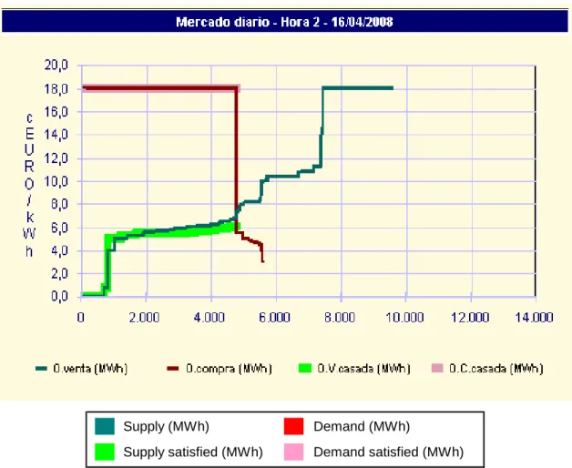
On Figure 1 we can see the market curves for Portugal for hour 2 of April 16, 2008. The extreme inelasticity of demand is clearly seen. The inelasticity of supply is not that notorious:
Figure 1: Supply and demand of energy for Portugal - hour 2 of April 16, 2008
Supply (MWh) Demand (MWh)
Supply satisfied (MWh) Demand satisfied (MWh)
“Another distinguishing feature of electricity markets is the potential for suppliers to exercise market power”2 (Knittel and Roberts, 2005: 794). This oligopolistic nature is characterized by a few dominant players, even in markets where it seems to exist enough competitors to produce lower prices (Bunn and Karakatsani, 2003).
The presence of negative prices can actually happen in power markets, as for some generators may be more profitable to pay so that a plant would not get off the system for one or two hours (which would increase the production marginal cost due to the start up cost).
In MIBEL that is not allowed as the minimum bid level allowed is 0 €/MWh.
2
In a report published in May 2009, by the Portuguese Competition Authority about the gross prices’ formation in Portugal in the second semester of 2007, the Authority concludes that there were evidences that support that EDP Produção (the main electrical company in Portugal in the gross market) in more than 80% of the hours was indispensable to satisfy at least 25% of the demand (and in 22% of the period EDP was necessary to supply more than half of the demand)
Based on this brief introduction, the main purposes of this thesis are: forecasting the day-ahead electricity prices for the Portuguese Power Market through ARIMA models, and comparing two different approaches. A first one in which the complete hourly prices time-series is used to forecast short-term prices through a selected ARIMA model and a second one where the price of each hour is independently forecasted leading to 24 independent analysis (and forecasts) of the 24 daily prices.
Electricity prices in the Portuguese Power Market, have not yet been studied before (also because no more than 3 years passed since the complete market opening)
We will use the Mincer-Zarnowitz regression and the Harvey-Newbold statistical test to enrich the study bringing a new perspective to the results as the forecasts were set against the real values and the models were compared to each other before selecting the best one.
To perform an hour-by-hour analysis (after Cuaresma et al. (2004)), intended to bring some accuracy to the forecasts as we could treat each one of the 24 price series as a “regular” time-series while the complete time-series had to take into account previous forecasts in order to get new forecasts.
The thesis is organized as follows. Next section presents the literature review with the most important conclusions resulting from the econometric approaches done on the subject. Section 3 describes the ARIMA models used in this study, for the complete time-series analysis and the hour-by-hour analysis. Section 4 discusses estimation results and compares out-of-sample evaluation for an Autumn and a Summer period. Finally, section 5 presents some concluding remarks.
2. LITERATURE REVIEW
Although being a recent research subject the study of the electricity prices’ series throughout the world (only possible after the markets’ deregulation) has produced several diversified papers in the last fifteen years.
Because each market has its own rules, not every detail in each study can be blindly applied to all markets. Even so, because all power markets share a kernel of important characteristics (mentioned above), the methods and the conclusions already published can be generally applied to the liberalized markets.
As the scientific papers related with the Portuguese energy market are very sparse or do not exist, and due to the main objective of this thesis, forecasting the energy prices in the Portuguese market, the analysis of prior research is oriented for the econometric tools already used to forecast energy prices considering different time frequency and/or different markets.
Nogales et al. (2002) presented two forecasting tools, based on time-series
analysis, with similar econometric background: dynamic regression and transfer function models applied to the hourly price series in the Californian and Spanish markets. In both models a single fundamental was used: the demand. They found that the Spanish prices were less predictable as the daily mean error was about 5% against a 3% one for the Californian prices.
Huisman and Mahieu (2003) tried a different econometric approach: taking into account the mean-reversion, high volatility and the extreme spikes of electricity prices, a three states’ regime-switching model was proposed. The daily spot price (the average of the 24 hourly prices in each day) was decomposed as the sum of a deterministic and a stochastic component, in which mean-reversion can be separated from spike periods. Three markets’ data were used for comparison purposes (APX from The Netherlands, LPX from Germany and Telerate UK Power Index).
Contreras et al. (2003) suggested two kinds of ARIMA methodologies to
forecast day-ahead prices in the Californian and Spanish markets again: a pure ARIMA model and an ARIMA model with two exogenous explanatory variables: the demand and the available daily production of hydro units. The average daily mean error in the Spanish market was about 10% while in the Californian market was about 11%.
A summary of the research done on the power markets was made by Bunn and Karakatsani (2003) in a working paper where the fundamentals of power markets and the behaviour of electricity prices have been organised and explained.
Cuaresma et al. (2004) based their empirical study on the hourly prices of the
LPX market. The methods applied include AR and ARIMA models, with time-varying intercept or jumps (ARIMA). They concluded that “an hour-by-hour modelling strategy
for electricity spot-prices improves significantly the forecasting abilities of linear univariate time-series models” (Cuaresma et al., 2004: 105)
Guirguis and Felder (2004) studied historical electricity prices from two New York State areas to conclude about the forecasts’ improvement of GARCH models
when compared to other techniques such as dynamic regression, transfer-function models and exponential smoothing.
Conejo et al. (2005) compared the three time series’ methods they had worked on before (ARIMA, dynamic regression and transfer function) with neural networks and wavelets. The demand was considered as exogenous variable but not always improved the forecasts’ accuracy. Transfer function and Dynamic regression presented the best predictions on the PJM Interconnection.
Knittel and Roberts (2005) presented a comparative study of several forecasting methods applied to electricity prices (a mean-reverting process (AR), Jump-diffusion, ARMA with time-varying intercept (ARMAX), EGARCH or ARMAX with temperature as exogenous variable). ARMAX, EGARCH and Jump-diffusion were among the models with the best performances suggesting a malleable statistical behaviour of electricity prices, the presence of spikes and time-varying high volatility. The data consisted of hourly prices from California.
Nogales and Conejo (2006) returned with a detailed analysis of the electricity hourly prices’ forecast through transfer function analysis. Demand data was used as the unique explanatory variable for forecasting in the PJM Interconnection.
Huisman, Huurman and Mahieu (2007) proposed a very different approach. In this paper “hourly prices cannot be seen as a pure time series process” (Huisman and Huurman, 2007: 242) as time-series models assume the information is available in each time step and not every 24 time steps. To forecast the price for hour 23 of the next day, we just know the prices until hour 24 of the previous day and not the one from hour 22 of the next day. A panel-data analysis is suggested in which the prices of 24 cross-sectional hours vary from day to day. Three data sets were compared: APX, EEX from Germany and PPX from France.
Silva (2007), in her Master Thesis, provided a comparative study of statistical models to predict electricity prices. She studied short-term forecasts both for daily and monthly prices. For the day-ahead prices forecast, SARIMA models and GARCH models were tested while for the next-month prices forecast, the approach was made through SARIMA models, SARIMA with intervention effects and GLS (Generalised Least Squares) models. The OMEL Spanish prices were the working data. The GARCH model was the one that performed better.
Weron and Misiorek (2008) compared several forecasting tools ending up for concluding that, although not being unanimous, a semiparametric approach (an Auto
Regressive model calibrated with a smoothed nonparametric maximum likelihood estimator) had a better performance than AR, Regime-Switching or Mean-reverting jump diffusions models. Californian and Nord Pool’s hourly prices constituted the working data.
Bunn and Karakatsani (2008) came up with an exhaustive study of the UK market. After realizing that stochastic models were incomplete (good for modelling but not so good for forecasting) and that the existing models are more concerned about the autoregressive effects than price’s reaction to fundamentals, a large comparative study of models, with a large number of explanatory variables was suggested. Time-varying parameters, either a Regression or Autoregressive, were the most accurate.
No more than twenty years ago, worldwide liberalized power markets only existed as projects and nice political intentions. When they boomed, several econometric tools found in electricity prices a new object to test their own reliability. Much more work on the subject will be produced in the coming years, as the existing markets will eventually be getting into their maturity. As we will see in the next sections, this work is also a contribution for comparing two energy prices forecasting techniques.
3. METHODOLOGY
3.1 Models and frequency data
Following several power markets’ researchers (Contreras et al. (2003), Cuaresma et al. (2004), Conejo et al. (2005)), I have the purpose to build a model which will able to forecast the 24 day-ahead electricity prices. For this purpose, and according to the literature review, a great number of options came up. The reasons that led me to forecast electricity prices through ARIMA models come in the next paragraphs.
As it is explained in APPENDIX A, both the Portuguese and the Spanish markets are related (even physically) so, predicting prices for these markets should be an interesting study (probably an idea for future research). Anyway, as some work has already been done on the Spanish market, which exists since 1998 (Contreras et al. 2002
and 2003) and no public work has been published about the Portuguese market (at least in the econometric point of view), I decided to concentrate on the Portuguese case.
After some research, and based on the literature review, I realized the large number of different approaches which had already been applied to the subject (Simple regressions, GARCH-type models, ARIMA models, ARIMA models with exogenous variables, Jump-diffusion models, Markov-processes’ models, exponential smoothing, transfer-function models, neural network models, etc...).
While looking for fundamentals that are significant to predict the hourly electricity prices, a restricted number of variables always appeared: temperature, level of the reservoirs and demand. However, two main problems arise when these variables are included: in an hour-forecasting model, we need both hourly-basis historical data and forecasts for the explanatory variables, which may not be available or may have a considerable error component. The more fundamentals we include in the model, the larger error component we may get (Weron, 2006). For example, if we think about hourly temperature forecasts for the next 30 days, we realize the enormous potential error in perspective, besides the difficulties in getting access to historical hourly data. With demand, although historical information is freely available, the greatest problem is due to its forecast3. Furthermore, pure time series models are more appropriate to describe the behaviour of power markets than of financial markets, due to the “normal” seasonality, which occurs with the electricity prices (Weron, 2006).
Based on this, I decided do not include any of these fundamentals in the estimated models. I assumed that general fluctuations in demand and temperature are already incorporated in historical prices; otherwise, as we forecast the price for each hour of the 30 days-ahead, we would have to include 720 point forecasts (30 x 24) per fundamental variable included in the model.
The unique variables I added to the standard ARIMA model are three dummy variables, which have been included one-by-one separately. The first dummy captures the weekend effect (being 1 on Saturdays and Sundays and 0 on working days), the second dummy captures the holiday effect (being 1 on holidays, if not a weekend, and 0
3
In the Portuguese Competition Authority’s report published in May, 2009, it is explained that the demand forecast relies, among other things, in the forecast of eolic energy production which is highly volatile once it depends directly from the wind speed and direction in each hour.
otherwise) and the third dummy grouped the previous two (being 1 on weekends and holidays and 0 on the remaining days).
I also considered to exclude weekends (because prices are much different from the remaining weekdays) and to include a dummy variable to capture the effect of each one of the four seasons. However, I did not realise any of these changes. It seemed to me that, excluding weekends would change the prices relation pattern in such a way that some important inference could be lost in the process. Including a variable to reflect the seasonal effect seemed useless once it would only make sense in a large sample (more than a year) so that the seasonal cycle could be captured.
My initial idea was also to include a volatility analysis to the Portuguese electricity hourly prices and so, to include the possible ARCH effects in the model. Guirguis and Felder (2004) concluded that GARCH models performed better than other statistical ones and Knittel and Roberts (2005) found evidence of an “inverse leverage effect” in electricity prices. Because this is not a closed research, my next step in this investigation will be to test the significance of ARCH effects and to analyze the electricity prices considering conditional heteroskedastic models. Anyway, I performed the log-transformation to the data in order to prevent some time-varying volatility.
One of the improvements of this work is that it considers the complete time-series analysis at once but also analyses each hour separately (hour-by-hour analysis). Cuaresma et al. (2004) concluded that an hour-by-hour analysis performed more accurate forecasts than if one considers the complete hourly time-series at once. Furthermore, in each case, the kind of prediction should be different. As Huisman, Huurman and Mahieu (2007) refer, if we consider the real hourly price formation process, the complete series is not a “normal” time-series once we do not know the value of an observation at each time step, but all the 24 at once every 24-length cycle. This impacts directly the forecasts’ method and consequently, its quality.
By using the complete series, prediction must be obtained day-by-day and we must use forecasts in order to produce new forecasts. For example, to forecast the price for the hour 24 of the next day, we don not know the prices of the first 23 hours of that day. So, we should run the model in order to get the forecast price for hour 1, and then we use that forecast to forecast the price for hour 2, and so on. When we get the forecasting for hour 24, the previous 23 observations are not real values but forecasts.
The hour-by-hour analysis has the advantage of eliminating this issue. Because we consider 24 separate time series, one for each hour, when we will perform the forecast of the hour 24 of the next day, we only use the series of prices of hour 24 from previous days. Thus, we know the real value of past observations and no forecasts are needed to perform a new forecast. In the EViews program, in the former case we must perform a dynamic forecast every 24 observations for the whole 720 forecasting period, and in the later one, we can perform a static forecast for the whole 30 observations of the forecasting period, for each one of the 24 models. I performed both so I could compare which one produces best results.
3.2 Estimation and forecasting periods
In terms of sample size, and from the information we could get, there is not one best standard estimation period. Nogales and Conejo (2006) used only 61 days (in a complete time series approach which completes 1,464 observations), Weron and Misiorek (2008) used a 9 months sampling period, Bunn and Karakatsany (2008) used almost 10 months (300 days) and Knitell and Roberts (2005) considered 29 months (21,216 observations). Based on this, I decided to consider a 6 months sampling period in order to get forecasts for the next 30 days. More than that seemed to be excessive: I thought that it would not improve the model’ performance once it would capture price relations too far from the present time (in dynamic markets, where the production mix is changing regularly, it is expected that the price relation over time becomes dynamic too).
As some researchers evaluated their models in different periods, usually in the more stable and more volatile ones (Weron and Misiorek, 2008; Nogales et al., 2002), the same methodology was adopted. We selected two 30-days forecasting periods, the first in the Autumn of 2008 and the other in the Summer of 2009 (actually it wasn’t exactly a Summer season, since June is a half-Spring and a half-Summer period).
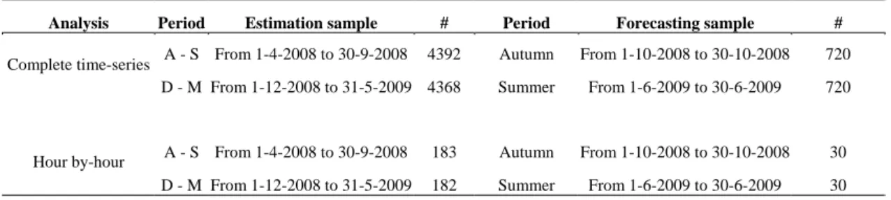
Therefore, the sample is partitioned in two distinct parts: the first part of the sample (6 months) is retained for the ARIMA parameters estimation while the remaining part (1 month) is considered as the forecasting period. In each part of the sample, we considered two distinct periods: April-September (A-S) and December-May
(D-M) for the parameters estimation and Autumn and Summer for the forecasting evaluation as one can see in table 1.
Table 1 Sampling periods
Analysis Period Estimation sample # Period Forecasting sample # A - S From 1-4-2008 to 30-9-2008 4392 Autumn From 1-10-2008 to 30-10-2008 720 Complete time-series
D - M From 1-12-2008 to 31-5-2009 4368 Summer From 1-6-2009 to 30-6-2009 720
A - S From 1-4-2008 to 30-9-2008 183 Autumn From 1-10-2008 to 30-10-2008 30 Hour by-hour
D - M From 1-12-2008 to 31-5-2009 182 Summer From 1-6-2009 to 30-6-2009 30
Parameters for the conditional mean equation are therefore estimated based on 6 months information (corresponding roughly to 183 and 182 observations in the hour-by-hour analysis and to 4,392 and 4,368 in the complete time-series analysis, for the A-S and D-M periods, respectively). These parameters are used to estimate the hourly conditional mean. To estimate the ex-ante out-of-sample predictive power of the models, the estimated parameters are used to forecast the hourly day-ahead conditional mean for the forecasting month (corresponding to 30 observations in the hour-by-hour case and 720 observations in the complete time-series analysis).
In the Autumn forecasting, there was some risk in considering an estimation period that began only 9 months after the Portuguese market’s opening. It may not have reached the required maturity level in order to produce a meaningful model. Anyway, some authors did not consider any “maturity-lag” at all (Cuaresma et al., 2004; Knittel and Roberts, 2005) and I decided to estimate the model based on that sample.
In the Summer case, the estimation period begins more than one year after the market opening. Thus, the market was at a different stage of maturity.
Another methodological issue was to decide if the estimating period would evolve over time. Most researchers applied the “Rolling Window” and the “Jackknife” methods. The “Rolling Window” method consists in, at each estimation step, to move one observation forward the calibration sample. The sample dimension remains unchanged. In the “Jackknife” method, only the ending observation would move forward at each step and the starting observation is the same at each step. So, the estimation sample dimension increases with time. The third option consists in keep the sampling period unchanged at every step: we estimate the model with a sample until a
certain day, and use that same model to forecast the prices for all the days of the forecasting period. I decided for this third option.
I started by applying all the three methods but I abandoned this idea for one main reason: some researchers (but not all) who used one of the two dynamic samples, usually made forecasts for longer periods (50 days or more) than the one I used (30 days). I believe that, in 30 days, the price relation through the days doesn’t change so dramatically that one needs to re-estimate the model at every time step.
Therefore, I decided to keep the forecasting period in a medium-size period (it seemed to me that 30 days fulfilled this condition) and to keep the model constant while forecasting through the 30 steps of the test sample.
As one can see in Figure 2, electricity prices behaved regularly in the OMEL during the two estimation periods (A-S and D-M).
Actually, there were not many values that one might consider as spikes: in fact there was only one extreme value (jump) in the sample, on February 2, 2009, on hour 5: the price reached 1 €/MWh (the average price from January to June 2009 was 40.88 €/MWh) as it can be seen in Figure 2. This observation was not deleted from the sample as jumps must be taken into account while working with electricity prices. If a larger number of jumps were observed in the sample, they should be treated carefully because, as Weron (2006) argues, one should be careful in handling the anomalous prices (usually spikes). Although one does not want to bias the price prediction with an outlier, the fact that spikes are actually important in power markets makes them non-excludable and so, they require a special attention.
Figure 2: The Portuguese electricity hourly prices - January 1, 2008 to June 30, 2009
0,00 20,00 40,00 60,00 80,00 100,00 120,00 01-01-2008 01-04-2008 01-07-2008 30-09-2008 30-12-2008 31-03-2009 30-06-2009 P ric e ( € /M W h )
The grey areas in Figure 2 are the forecasting periods: the Autumn one (October 2008) and the Summer one (June, 2009).
The only change performed on the series was the one in the missing hour in March (at the Spring’s starting) and the extra hour in October (when the Autumn starts). In the first case, I added one hour with the average price of both the previous and the following prices. In the second case, the 25th price of the day was eliminated to the series.
3.3 Econometric approach
In order to stabilize the variance and to reduce the heteroskedasticity impact on estimation results, the workable series are the natural logarithm of electricity spot prices.
Either in the complete time-series analysis or in the hour-by-hour analysis, I had to guarantee that the series was (at least) covariance stationary. To check the existence of a unit root and to test the stationarity of the series, the Augmented Dickey-Fuller (ADF) was performed. In the test equation, trend and intercept were included so that the test could capture not only the stochastic trend but also the deterministic trend of the series. An automatic lag length selection has been applied by using Schwarz’s Information Criterion (SIC) (more demanding than the Akaike Information Criterion (AIC) in what the number of estimated parameters are concerned).
When the null hypothesis of the ADF’s test applied to the electricity log-prices was not rejected, a first difference was computed and with this transformation, the new series became stationary. By the inspection of the estimated Autocorrelation Function (ACF) and Partial Autocorrelation Function (PACF), in some cases a seasonal differentiation is suggested and computed. However, this procedure is adopted only when, after performing a first order regular differentiation, the series remained non-stationary.
We expected that some seasonal behaviour might occur, specially a weekly effect, and by the ACF and PACF inspection, most of the analysed series seemed to
confirm this suspicion. Thus, based on the estimated autocorrelation functions we use ARIMA and/or SARIMA models for each considered period.
In the complete time-series analysis, a few times 24-length cycle emerged, while in the hour-by-hour analysis, a 7-length cycle was dominant (in the hour-by-hour analysis, the weekly effect is more evident than in the complete-time series where the daily cycle dominates).
In order to capture the weekly seasonal effect that SARIMA model could not capture and/or to capture the possible holiday effect, the three dummy variables mentioned earlier have been included in each one of the models separately.
After estimating the models, an autocorrelation residual analysis was performed based on Breusch-Godfrey LM serial correlation test. The test decision should point to a white noise process to assure that the estimated model was able to capture the observed linear dependency in the time-series data.
At this point, I had 2 groups of models (covering the A-S and D-M periods) each one divided in 25 subgroups: one for each of the 24 hours of the day and one for the complete time series’ analysis. A total of 507 models were estimated as several models have been considered for each one of the 25 subgroups, due to the Autocorrelation and Partial Autocorrelation functions appearance.
After estimation, the models’ selection began. The first criterion was to exclude any model with at least one pair of coefficient estimates with correlation greater than 0.7 (Murteira, 2000). This prevented that a small change in the estimation sample might cause a large difference in the model’s coefficients estimates (butterfly effect). By imposing this limitation, the number of candidate models diminishes to 339 models.
On the next selection step, the Mincer-Zarnowitz regression equation is estimated. The observed hourly electricity price from the Autumn and Summer 30-days forecasting period is the dependent variable in a linear regression having the forecasted values as the unique independent variable; intercept is also included in the regression. The purpose is to select from each one of the 50 subgroups, the 5 models with the highest coefficient of determination (R2) resulting from the Mincer-Zarnowitz regression. If in a subgroup there are less than 5 models, all of them are selected. At this step, 208 models remained after the Mincer-Zarnowitz regression was applied.
At this point, the Mean Absolute Error (MAE), the Root Mean Square Error (RMSE) and the Mean Absolute Percentage Error (MAPE) have been computed for the
208 selected models. The main reasons to compute these measures were to compare the hour-by-hour results with the ones resulting from the complete time series’ analysis and to compare this empirical study’s results with the ones from previous studies.
To select the best model from each one of the 50 subgroups resulting from the Mincer-Zarnowitz regression, the final criterion is the Harvey-Newbold (Harvey and Newbold, 2000) encompassing test. This test compares at once one single model (that we represent by model A, for example) with all the others, indicating if model A is better than the remaining ones. The test is based on a linear regression where the forecasting errors from model A is the dependent variable and the differences between the forecasting errors of model A and the ones resulting from the other models constitute the explanatory variables. In the null hypothesis, we state that model A encompasses the rest of the models under comparison against the alternative that at least one of the other models encompasses model A too. There are as many HN test results as models under comparison.
As the final criterion is the Harvey-Newbold test, the best scenario was to accept the null hypothesis in one of the forecasting models test and to reject it for all the rest of the models. Unfortunately, it might happen that none of the models encompasses all the others. In this case, the models selection is based on the highest p-value associated with the HN test result. Another possible scenario (and more plausible) is that several models encompass the remaining ones. If this is the case, the one that is more distant from the “rejection point” is chosen.
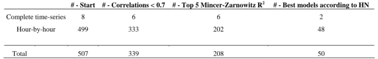
At this point 50 models were selected and Table 2 concludes about the number of models selected in each step.
Table 2: Number of models selected
# - Start # - Correlations < 0.7 # - Top 5 Mincer-Zarnowitz R2 # - Best models according to HN
Complete time-series 8 6 6 2
Hour-by-hour 499 333 202 48
4. EMPIRICAL STUDY
4.1 THE DATA
As we referred before, the sample used for parameters estimation is partioned in two different periods (from April 1, 2008 to September 30, 2008, A-S period, and from December 1, 2008 to May 31, 2009, D-M period) corresponding roughly to 183 and 182 observations in the hour-by-hour analysis and to 4,392 and 4,368 observations in the complete time-series analysis, for the A-S and D-M periods, respectively.
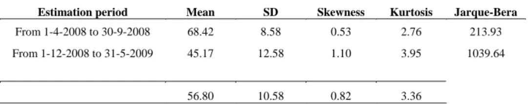
Table 3 shows the electricity spot prices descriptive statistics for the two estimation samples when the complete time-series analysis is considered. Tables 4 and 5 show the electricity spot prices’ descriptive statistics for the hour-by-hour analysis. The grey areas in the Jarque-Bera statistical test column indicate the hourly prices series where the normality assumption can be assumed (for 5% significance level).
Table 3: Descriptive Statistics for the Portuguese electricity spot prices (complete hourly series)
Estimation period Mean SD Skewness Kurtosis Jarque-Bera From 1-4-2008 to 30-9-2008 68.42 8.58 0.53 2.76 213.93 From 1-12-2008 to 31-5-2009 45.17 12.58 1.10 3.95 1039.64
56.80 10.58 0.82 3.36
In average, the prices were much higher in the period April-September (with an average difference greater than 20€/MWh) as 2008 was an extreme year in what concerns the electricity prices (Table 3). In terms of prices normality distribution, the hypothesis is rejected for both periods according to the Jarque-Bera test.
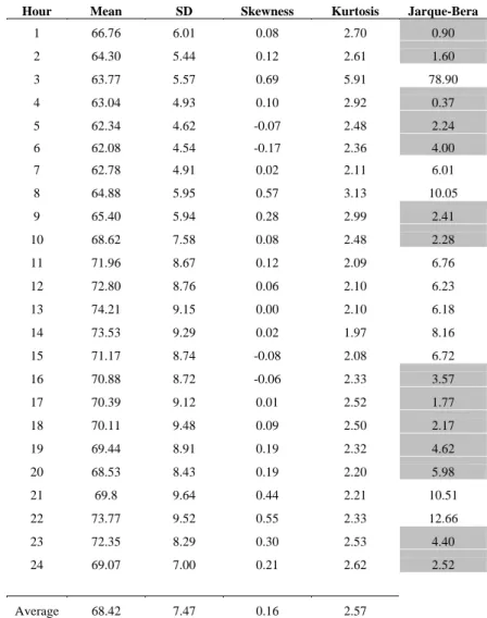
Table 4: Descriptive statistics for the Portuguese electricity spot prices over period April 1, 2008 to September 30, 2008
Hour Mean SD Skewness Kurtosis Jarque-Bera
1 66.76 6.01 0.08 2.70 0.90 2 64.30 5.44 0.12 2.61 1.60 3 63.77 5.57 0.69 5.91 78.90 4 63.04 4.93 0.10 2.92 0.37 5 62.34 4.62 -0.07 2.48 2.24 6 62.08 4.54 -0.17 2.36 4.00 7 62.78 4.91 0.02 2.11 6.01 8 64.88 5.95 0.57 3.13 10.05 9 65.40 5.94 0.28 2.99 2.41 10 68.62 7.58 0.08 2.48 2.28 11 71.96 8.67 0.12 2.09 6.76 12 72.80 8.76 0.06 2.10 6.23 13 74.21 9.15 0.00 2.10 6.18 14 73.53 9.29 0.02 1.97 8.16 15 71.17 8.74 -0.08 2.08 6.72 16 70.88 8.72 -0.06 2.33 3.57 17 70.39 9.12 0.01 2.52 1.77 18 70.11 9.48 0.09 2.50 2.17 19 69.44 8.91 0.19 2.32 4.62 20 68.53 8.43 0.19 2.20 5.98 21 69.8 9.64 0.44 2.21 10.51 22 73.77 9.52 0.55 2.33 12.66 23 72.35 8.29 0.30 2.53 4.40 24 69.07 7.00 0.21 2.62 2.52 Average 68.42 7.47 0.16 2.57
In what concerns the hour-by-hour analysis, the average electricity spot price is also higher during the April-September period for the daily 24 hours. The normality assumption only stands in 14 hourly price series of this period. The same assumption is always rejected for the 24 hourly series of the December-May period as one can see in Table 5.
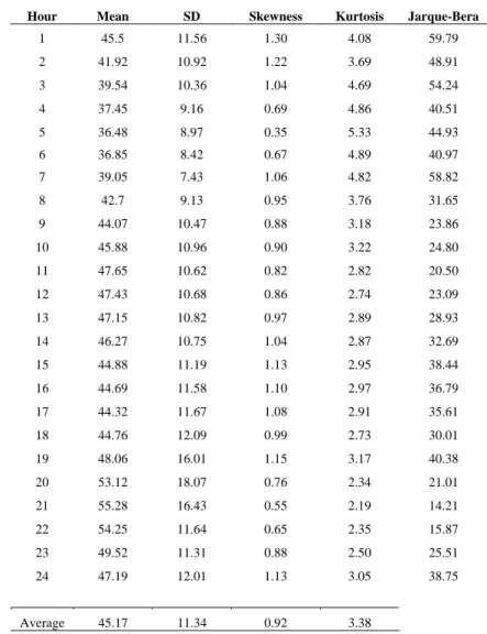
Table 5: Descriptive statistics for the Portuguese electricity spot prices over period December 1, 2008 to May 31, 3009
Hour Mean SD Skewness Kurtosis Jarque-Bera 1 45.5 11.56 1.30 4.08 59.79 2 41.92 10.92 1.22 3.69 48.91 3 39.54 10.36 1.04 4.69 54.24 4 37.45 9.16 0.69 4.86 40.51 5 36.48 8.97 0.35 5.33 44.93 6 36.85 8.42 0.67 4.89 40.97 7 39.05 7.43 1.06 4.82 58.82 8 42.7 9.13 0.95 3.76 31.65 9 44.07 10.47 0.88 3.18 23.86 10 45.88 10.96 0.90 3.22 24.80 11 47.65 10.62 0.82 2.82 20.50 12 47.43 10.68 0.86 2.74 23.09 13 47.15 10.82 0.97 2.89 28.93 14 46.27 10.75 1.04 2.87 32.69 15 44.88 11.19 1.13 2.95 38.44 16 44.69 11.58 1.10 2.97 36.79 17 44.32 11.67 1.08 2.91 35.61 18 44.76 12.09 0.99 2.73 30.01 19 48.06 16.01 1.15 3.17 40.38 20 53.12 18.07 0.76 2.34 21.01 21 55.28 16.43 0.55 2.19 14.21 22 54.25 11.64 0.65 2.35 15.87 23 49.52 11.31 0.88 2.50 25.51 24 47.19 12.01 1.13 3.05 38.75 Average 45.17 11.34 0.92 3.38
4.2 ESTIMATION AND FORECASTING RESULTS
The empirical results are shown in several tables. They are based on the information settled at the end of the first step before any selection criterion being applied. So, the results reflect the characteristics of all the 507 models mentioned above.
4.2.1 Complete time-series analysis
4.2.1.1 Stationarity
Based on the Augmented Dickey-Fuller (DF) test we concluded that both series are non-stationary. For the D-M series, a first regular differentiation was performed
while for the A-S series, a first regular differentiation or a seasonal differentiation were enough to transform the series into a (weakly) stationary one.
Table 6: Stationarity of the complete time-series
Period # First difference Seasonal difference (24) Stationary series
April-September (A-S) 1 1 1 0
December-May (D-M) 1 1 0 0
Total 2 2 1 0
4.2.1.2 Estimation models
A total of 8 models were estimated in the complete time series analysis, 6 for the A-S period and 2 for the D-M period (Table 7).
Non seasonal models in the complete time series analysis refer to any model where the maximum lag in the autoregressive or moving average terms is lower than 24.
Five seasonal models refer to the A-S period while only one refers to the D-M period. Thus, 6 out of the 8 estimated models had at least one seasonal (daily) coefficient. This suggests the strong daily relationship between hourly electricity prices.
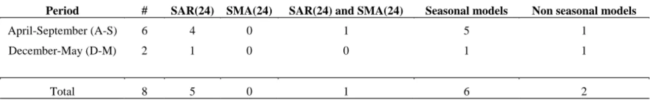
Table 7: Autoregressive and Moving Average lags per period for the complete time series analysis
Period # SAR(24) SMA(24) SAR(24) and SMA(24) Seasonal models Non seasonal models
April-September (A-S) 6 4 0 1 5 1
December-May (D-M) 2 1 0 0 1 1
Total 8 5 0 1 6 2
SAR: Seasonal Autoregressive, SMA: Seasonal Moving Average.
4.2.1.3 Dummy variables
First, I recall what the three dummy variables represent: Dummy is 1 on weekends and holidays and 0 otherwise, Weekends is 1 on weekends and 0 otherwise and Holidays is 1 on holidays and 0 otherwise.
The estimated coefficients for the dummy variables were statistically significant in just two of the 8 models and both for the A-S period as one can see in table 8.
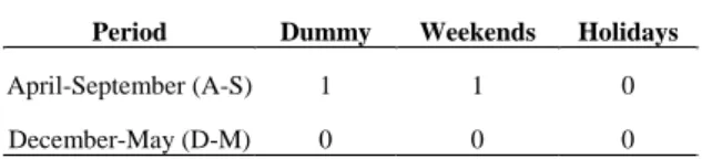
Table 8: The dummy variables in the complete time-series analysis
Period Dummy Weekends Holidays April-September (A-S) 1 1 0
December-May (D-M) 0 0 0
According to Table 9, although the estimated coefficients for the dummy variables representing both weekend and holiday effects, in one case, and the weekend effect in the other case, are statistical significant in seasonal models, no relevant conclusion can be taken as the cycle length represents one day (not one week).
Table 9: The relation between dummy variables and seasonality in the complete time series analysis
Seasonal models Non seasonal models
Period Dummy Weekends Holidays Dummy Weekends Holidays
April-September (A-S) 1 1 0 0 0 0
December-May (D-M) 0 0 0 0 0 0
4.2.1.4 The best model
For the A-S period, 4 models out of 6 reached the end of the process. The models with the dummy variables were among the best 4 and 3 of these models had a significant seasonal (daily) lag.
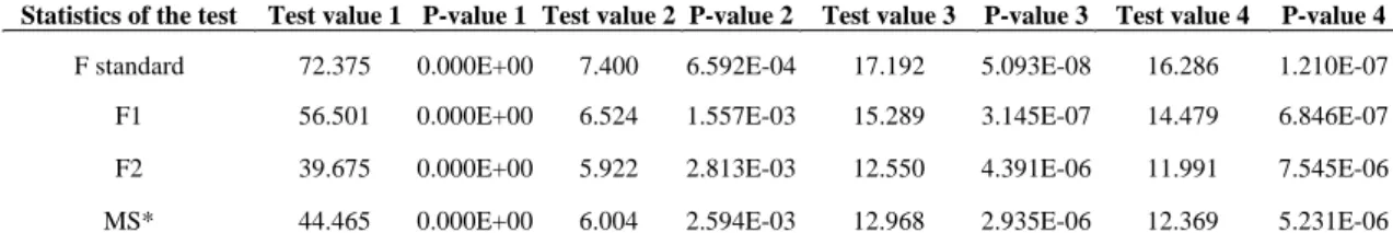
After performing the HN test4 (see the MS* row on table 10) the conclusions pointed to the rejection of the null hypothesis in spite of the model being considered; thus, none of the models encompassed the others. Due to these results, and based on the criteria defined before, the best model is the one with the HN test p-value closer to the significance level at 5%, which is, according to Table 10, model number 2. This model is a SARIMA (1,0,0)(1,1,0)24 with no dummy variables. This is the best forecasting
model for the 30-days in the Autumn season.
4
Table 10: The Harvey-Newbold test’s results for the A-S period on the complete time series analysis
Statistics of the test Test value 1 P-value 1 Test value 2 P-value 2 Test value 3 P-value 3 Test value 4 P-value 4 F standard 72.375 0.000E+00 7.400 6.592E-04 17.192 5.093E-08 16.286 1.210E-07 F1 56.501 0.000E+00 6.524 1.557E-03 15.289 3.145E-07 14.479 6.846E-07 F2 39.675 0.000E+00 5.922 2.813E-03 12.550 4.391E-06 11.991 7.545E-06 MS* 44.465 0.000E+00 6.004 2.594E-03 12.968 2.935E-06 12.369 5.231E-06
Next table presents the error forecasting measures resulting from the selected model.
Table 11: The error forecasting measures for the best model of the A-S period on the complete time series analysis
Model MAE RMSE MAPE SARIMA (1,0,0)(1,1,0)24 3,87 5,10 5,15%
Based on MAE, RMSE and MAPE results (MAE and RMSE are measured in €/MWh whenever they appear in this document), we conclude that the values are in line with the ones from previous studies.
In Summer forecasting period, 2 models rested in the final step: ARIMA (0,1,1) and SARIMA (0,1,0)(1,0,0)24. None of them has a significant dummy variable.
The MS* line from Table 12 shows the HN test results. Model number 2, a SARIMA (0,1,0)(1,0,0)24,emerged as the best model.
Table 12: The Harvey-Newbold test’s results for the Summer period on the complete time-series analysis
Statistics of the test Test value 1 P-value 1 Test value 2 P-value 2 F standard 295.784 0.0000 0.132 0.7161
F1 277.980 0.0000 0.124 0.7244
F2 130.653 0.0000 0.124 0.7244
MS* 159.396 0.0000 0.124 0.7245
The common forecasting accuracy measures for the best model are presented in table 13. The results are slightly higher than the ones I expected. For example, the value for MAPE (9%) is higher than the expected 7%-7.5%.
Table 13: The error forecasting measures for the best model of the Summer period on the complete time-series analysis
Model MAE RMSE MAPE
SARIMA (0,1,0)(1,0,0)24 3,39 4,45 9,02%
Surprising was the fact that the MAPE for the Summer forecasting period was much higher than the one in the Autumn season. However, these results are in line with the ones of Contreras et al. (2003).
One final point to refer is that these results were achieved with a daily dynamic forecasting, which means that, in each day, the forecasting procedure for the next day is based on forecasts for that same day and not on real data. For example: to forecast hour 10, hours 1, 2, ..., 9 are forecasts and not real values as they are not known at the forecasting moment.
4.2.2 Hour-by-hour analysis
Hour-by-hour analysis is also conducted in four steps: Stationarity of the series, Estimation models, Dummy variables and Best model selection.
4.2.2.1 Stationarity
Based on the Augmented Dickey-Fuller tests and Table 14 results, we can conclude that most of 24 hourly series are non-stationary in spite of the A-S or D-M period being considered. In the D-M period, 23 hourly series are non-stationary, while in the April-September period all the series are non-stationary. The necessary transformation to achieve the stationarity of the series is not always the same, but in 90% of the series, a first regular differentiation was enough. In three cases, it was necessary a regular and a seasonal differentiation to produce stationary transformed time series and in just one case, a seasonal differentiation turned the series into a stationary one.
Table 14: Stationarity of the hourly time series
Period # First difference
Seasonal difference (7)
First difference and seasonal difference (7) Stationary series April-September (A-S) 24 22 1 1 0 December-May (D-M) 24 21 0 2 1 Total 48 43 1 3 1 % 89.6% 2.1% 6.3% 2.1% 4.2.2.2 Estimation models
Based on Table 15 results, we conclude that from the 499 estimated models in the hour-by-hour analysis, 277 are used to forecast the electricity prices for the Summer period while the remaining 222 models produce the Autumn prices forecasts.
Table 15: Autoregressive and Moving Average lags per period on the hour-by-hour analysis
Period # SAR(7) SMA(7) SAR(7) and SMA(7) Seasonal models Non seasonal models
April-September (A-S) 222 68 55 66 189 33 December-May (D-M) 277 41 54 95 190 87 Total 499 109 109 161 379 120 % 76.0% 24.0%
SAR: Seasonal Autoregressive, SMA: Seasonal Moving Average.
In spite of the period being considered, April-September or December-May, more than 75% of the estimated models had at least one (weekly) seasonal component (189 and 190 models, representing 85% and 69%, respectively). Thus, the seasonal component of the Portuguese electricity prices is stronger in the hour-by-hour analysis when compared to the complete time series approach.
4.2.2.3 Dummy variables
Table 16 refers to the presence of the dummy variables in the estimated models. From 499 models, 202 include a dummy variable (40.5%) whose estimated coefficient is statistically significant. This number reflects the importance of these variables as they complement the weekly behaviour (and/or holiday effect) on the prices series.
Table 16: The impact of dummy variables on the hour-by-hour analysis
Dummy Weekends Holidays Total
Period # # % # % # % # %
April-September (A-S) 222 26 11.7% 22 9.9% 16 7.2% 64 28.8% December-May (D-M) 277 59 21.3% 41 14.8% 38 13.7% 138 49.8%
Total 499 85 17.0% 63 12.6% 54 10.8% 202 40.5%
Analysing each one of the three binary variables, the most representative is the
Dummy which refers to the weekend and holiday effects (it is included in 17% of the
estimated models). The weekend effect comes next with Weekends representing roughly 12.5% and Holidays comes lastlty, included in 11% of the models. This decreasing frequency of the dummy variables (from Dummy to Holidays) occurs either in the A-S or in the D-M periods.
As one can see (Table 16), the presence of these variables is more significant in the December-May period where almost 50% of the estimated models include a dummy variable, while in the April-September period that percentage reduces to 29%.
The hour-by-hour analysis results in a larger percentage of statistically significant dummy variables coefficients when compared to the complete series analysis. This can be explained by the fact that the hour-by-hour analysis considers 24 time-series, one for each hour: because in each one of the series, each observation corresponds to one unique day, different hours of the day have different dummy coefficients. In the complete time series analysis, the 24 hours of each day are considered in the same series. Thus, the dummy coefficient is the same for the whole 24 prices and so, this analysis might reduce its explanatory power.
In order to analyse the dummy variables effects in the seasonal and non-seasonal models, we aggregated the results in Tables 17 and 18.
Table 17: The dummy variables/seasonality relation in the hour-by-hour analysis
Seasonal models
Period # Dummy % Weekends % Holidays % Total % April-September (A-S) 189 23 12.2% 19 10.1% 14 7.4% 56 29.6% December-May (D-M) 190 40 21.1% 22 11.6% 31 16.3% 93 48.9%
Total 379 63 16.6% 41 10.8% 45 11.9% 149 39.3%
Within the seasonal models, more than 39% include a dummy variable. The weekend and holiday effect Dummy variable is the most frequent (it is included in 63 models, representing 16.6%). The holiday effect comes next with 11.9% of the models and finally the weekend effect appears in 10.8% of the models. Dummy is also the most frequent in both periods, but Weekends and Holidays switch positions: Weekends are more important than Holidays in the April-September period, but the opposite takes place in the second period. The dummy variables appear more often in December-May: 93 models representing almost 49%, against 29.6% for the April-September period.
Proceeding with the non-seasonal models (table 18), we conclude that the frequency of the Holidays dummy variable decreases when compared to its presence in the seasonal models (from 11.9% to 7.5%). The number of models with Dummy variables (weekends and holidays effects) increases slightly from 16.6% to 18.3% but the strong increase comes from Weekends dummy variable that appears in 18.3% of the models (versus 10.8% in the seasonal ones).
We expected this result as seasonal coefficients that previously captured the weekly effect, overpassed the Weekends coefficient. With no seasonal coefficients, the weekly effect should be captured through the Weekends variable.
Table 18: The dummy variables/non-seasonality relation in the hour-by-hour analysis
Non seasonal models
Period # Dummy % Weekends % Holidays % Total % April-September (A-S) 33 3 9.1% 3 9.1% 2 6.1% 8 24.2% December-May (D-M) 87 19 21.8% 19 21.8% 7 8.0% 45 51.7%