Of cities and slums

Of Cities and Slums

∗

Pedro Cavalcanti Ferreira

Alexander Monge-Naranjo

Luciene Torres de Mello Pereira

March, 2017

Abstract

The emergence of slums is a common feature in a country’s path towards urbanization, structural transformation and development. Based on salient micro and macro evidence of Brazilian labor, housing and education markets, we construct a simple model to examine the conditions for slums to emerge. We then use the model to examine whether slums are barriers or stepping stones for lower skilled households and for the development of the country as a whole. We calibrate our model to explore the dynamic interaction between skill formation, income inequality and structural transformation with the rise (and potential fall) of slums in Brazil. We then conduct policy counterfactuals. For instance, we find that cracking down on slums could slow down the acquisition of human capital, the growth of cities (outside slums) and non-agricultural employment. The impact of reducing housing barriers to entry into cities and of di§erent forms of school integration between the city and the slums is also explored.

Keywords: Skill formation; Locations; Occupations; Structural transformation. JEL Codes: O15, O18, O64, R23, R31.

∗_{The views expressed here are those of the authors and do not necessarily reflect the opinion of the Federal Reserve}

Bank of St. Louis or the Federal Reserve System.

†_{EPGE/FGV, Rio de Janeiro.}

‡_{Federal Reserve Bank of St. Louis and Washington University in St. Louis.} §_{EPGE/FGV, Rio de Janeiro.}

“What connexion can there have been between many people in the innumerable histories of this world, who, from opposite sides of great gulfs, have, nevertheless, been very curiously brought together!” Charles Dickens, Bleak House

“The new residents brought garbage, bins, mongrel dogs... poverty to desire wealth...legs for waiting for buses, hands for hard work, pencils for state schools, courage to turn the corner and...asses for the police to kick...” Paulo Lins, City of God: A Novel

1

Introduction

Structural transformation and urbanization are hallmarks in the development of countries.1 _Most

developed countries have all but completely displaced their workers from agriculture —and other primary sectors— towards manufactures and services. Recent work pushes the importance of this reallocation further by highlighting the emergence of high-skill services in later stages of

devel-opment.2 _{Since agriculture is predominantly a rural sector, and manufacturing and many service}

sectors are predominantly urban activities, then barriers to urbanization per se can easily translate into barriers to structural transformation and development, as emphasized by Lewis (1954) long ago. Likewise, forces that lead to structural transformation of countries can shape the urbanization patterns of countries, including the size and fragmentation of cities.

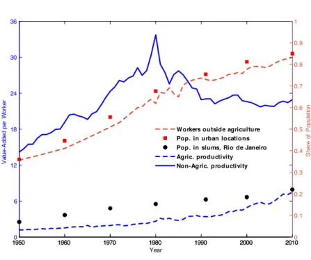
Urbanization, of course, has been rarely a smooth process. The story of the world’s leading cities —London, Paris, New York, Tokyo, etc— is in large measure the story of their slums. The emergence of these cities cannot be understood without putting considerable attention to the rise, expansion and eventual fall of slums, the lives of their dwellers, and the advancement of their descendants. More recently, since World War II, many developing countries have undergone transitions from rural to urban economies at a rapid pace. For instance, as shown in Figure 1, in Brazil, the fraction of the population living in urban areas increased from 36% in 1950 to 85% in 2010; by 1970 the country was already predominantly urban. Notice that the labor share in non-agricultural sectors closely follows the urban population, going from 36% in 1950 to 83% in 2010. Similar findings are observed in Mexico: between 1960 and 2010 the urban population rose from 51% to 88%, and the non-agricultural labor share went from 48% to 86%. South Korea was initially even more rural, but experienced a faster transformation. In the early 1960s, 72% of its population lived in rural areas and 62% of its workers were in agriculture. In 2010, the shares of urban population and non-agriculture labor were 93% and 82%, respectively.

Yet, underneath these common features of structural transformation, countries can exhibit dras-tic di§erences, in terms of output growth, forms of urbanization, social mobility and income dis-parities. For instance, since 1950, South Korea presents a sustained upward trend in its income per capita (and output per worker) relative to the U.S. Korean employment has shifted to high skill services. And in terms or urbanization, the slums in Seoul have all but disappeared. In contrast, Brazil, Mexico and quite a few other Latin American economies have stagnated since the early 1980s, falling further behind the U.S. in relative terms of output per capita. Non-agriculture labor productivity has been falling since 1980, because the employment expansion in those sectors has been mostly in low skill urban jobs, as we document below. Notably, the growth of the main cities in Brazil and Mexico has been driven in large part by the growth in the slum population. In these two countries, as well as in many others, migrants from rural areas have low levels of human capital and migrate to the urban areas to work in low skill jobs. Slums are the mechanism available to those migrants to avoid the housing costs of the formal city, and still access the urban labor markets.

1_{See for example the Nobel lecture of Kuznets (1973).}

In this paper, we propose a dynamic model with endogenous skill formation and heterogeneity to understand the di§erences in the urbanization and structural transformation patterns of countries. We guide the construction of the model and its calibration by our own exploration of the Brazilian experience. We examine the evidence about urbanization, formation of slums, and human capital accumulation across di§erent locations. Using the Brazilian Census we compute the evolution of population across rural and urban areas, and across slums and cities through the years. We also measure the population of migrants and non-migrants in slums and cities. Crucially, we explore what factors drive migration: the incomes, schooling attainment and inter-generational transitions of schooling attainment, conditional on locations.

We consider the simplest model that can be used to analytically examine: (i) structural trans-formation; (ii) urban development; (iii) income and skills distribution; (iv) social mobility. The key elements in the equilibrium are, first, how to allocate individuals and skills across locations, productive sectors and occupations and, second, the dynamic implications of those decisions for the skill formation of future generations. In our model, individuals can choose to live in rural or urban locations. The skill population is endogenously sorted across the locations of the country, and the human capital formation of children is determined by the location’s human capital. Al-truistic parents take into account the human capital formation of their children at the time they choose their location of residence. To live in the city people must buy a house, a form of fixed cost. Slums o§er the option of entering urban labor market and avoid housing costs, but this option comes at the cost of losses that are in direct proportion to the individual’s earnings. Whether urban locations exhibit slums or not depends on the predetermined skill dristribution, and is jointly de-termined with housing prices and the relative price of goods, which in the model are dede-termined by non-homothetic preferences as in recent models of structural transformation. We then analyze the equilibrium allocations in terms of the implied allocation of labor across sectors and occupations, the size of urban areas and their composition in terms of cities and slums. We then calibrate the model to the Brazilian economy, explore its ability to fit the key Brazilian data, and use it to explore the impact of alternative policies.

More concretely, we consider a discrete-time, infinite-horizon economy populated by dynasties of two-period-lived overlapping generations (OLG) of individuals. In any period the population of the economy is described by a positive measure over all positive levels of skills. The population remains constant, but its skill composition evolves over time. The economy has two production sectors, agriculture and non-agriculture (manufacturing and services), three locations: rural areas, favelas (slums) and city centers. There are three occupations: rural occupations (low skill) and urban occupations, which are qualified or skilled. Qualified occupations required a minimum skill level to be productive, while the urban skill occupations, there can be two groups: low-skilled urban jobs or high skilled urban jobs.

We show that the equilibrium in the economy can have two di§erent configurations: an equi-librium with only high skilled urban jobs and an equiequi-librium with urban low skilled services jobs, and examine the conditions under which these configurations arise. In particular, we highlight the importance of initial skill disparities and preference non-homotheticities to generate low skill urban jobs equilibria. We also highlight the role of housing costs and education concerns in generating slums equilibria. Finally, we highlight the importance of segmentation in the formation of education and potential rising costs for the persistence of low skill urban jobs and slums.

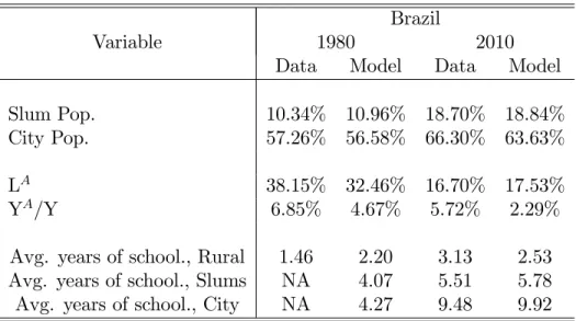
A calibration of our simple model can reproduce the evolution in the distribution of the Brazilian population across occupations and locations from 1960 to 2010. Using the model as a basis for examining counterfactual policies, we explore the impact of rising housing costs and of cracking down slums. We find that higher housing costs would increase the population in slums, but would not a§ect much the structural transformation of the country. In short, for low skill workers slums

appear to be good substitutes to formal city dwelling. However, the complete prohibition of slums would have slowed down substantially the structural change and the urbanization of the country, as only the most skilled individuals would a§ord to live in the cities.

The reminder of the paper is organized as follows. In the next section, we briefly discuss existent related literature. In Section 3, we examine the case of Brazil and highlight a number of salient facts about its structural transformation, urbanization and the emergence of slums. Section 4 sets out our model and defines equilibrium. Section 5 characterizes the equilibrium allocations in the model, and explore the conditions for the emergence of slums, and the impact of slums on the overall urbanization, structural transformation and growth of a country. Section 6 calibrates our model to the Brazilian experience from 1960 to 2010. Section 7 uses the model to explore the implications of di§erent policies: changes in the housing costs of cities, cracking down on slums, and the integration of schools systems. Section 8 concludes.

2

Related Literature

This paper is connected to two broad and related areas in the development literature, namely structural transformation and urban development. Both branches are very extensive, and a com-prehensive review would be well outside the limits of this paper. Hence, we will review only the most related papers and highlight the aspects most relevant for our analysis and findings.

With respect to the vast literature on structural transformation,3 _{our work is closest to papers}

that investigate episodes of accelerated growth, stagnation and decline, based on sectoral produc-tivity di§erences and reallocation. Buera, Kaboski and Rogerson (2015) find that increases in GDP per capita are associated with a shift to sectors that are high-skill labor intensive and further development leads to an increase in the relative demand for skilled labor.

Along the same lines, Duarte and Restuccia (2010) study the role of sectoral labor productivity in structural transformation and in the trajectory of aggregate productivity of 29 economies. They note that the catch-up process (relative to the United States.) in manufacturing productivity can account for about half of the productivity gains. As a counterpart, the low productivity —and lack of catching up— of the service sector explains the episodes of stagnation and decline. This work can be useful to understand the experience of countries that have stagnated. Indeed, Silva and Ferreira (2015) extend the analysis of Duarte and Restuccia (2010) for six Latin American economies in the period of 1950-2003. Using a four-sector model (agriculture, manufacturing, modern services and traditional services), these authors conclude that the poor performance of the traditional services sector is the main source of the slowdown in productivity growth after the mid-1970s in Latin America. Our paper here highlights that much of the expansion of non-agricultural production can occur in low-skills jobs, which would translated in observed low productivity, as we document for Brazil. Our simple model can be used to examine the conditions under which a country’s structural transformation is directed to high skills non-agricultural occupations or whether it will also be directed to low-skill ones.

At any rate, the reallocation from agriculture to non-agricultural sectors is strongly associated to the reallocation of workers from rural to urban areas. Indeed, the literature is strongly dominated by the view that urbanization, structural transformation and growth go together, partly because no single country has reached middle-income status without a significant population shift into

cities.4 _{Many papers emphasize the role of agglomeration economies, from cost advantages for}

workers and firms inside a city , such as linkages between industries, better infrastructures, network

3_{See the Handbook chapter by Herrendorf, Rogerson and Valentiny (2014).} 4_{See Figure 1.1 in Annez et al. (2009).}

externalities, thickness in labor and goods markets, etc. From this large and diverse literature we can only highlight the relationship with a number of papers. As in Lucas (2004), we model cities as fertile places for the formation of skills because of the exposure of ideas, a local public good whose level is endogenously determined in equilibrium. Contrary to Lucas (2004), learning opportunities within urban areas can be fragmented. Thus, our model is closely related to Benabou (1996), and Fernandez and Rogerson (1998), which examine models with human capital formation fragmentation in cities. The emphasis of those paper is in the implications of di§erent school reforms, while our focus is on the emergence of slums and the endogenous fragmentation of cities along the path of structural transformation and urbanization.

In our model, the emergence of slums is driven by housing costs, a form of congestion costs. Therefore, we connect to a substantial literature on congestion costs (negative externalities) and their e§ect on urbanization a§ects growth. These congestion costs can be illustrated by higher cost of infrastructure (piped water, sewage, electricity, transportation), high real estate prices (low supply of housing), pollution, and bad quality of social services (education, health). The literature points to the evidence that urbanization takes place in the early stages of development, often before economies have reached middle incomes status. Therefore, rural-urban migrants with low human capital accumulation and low income usually settle in squatter areas, an aspect that is central to our model.

A crucial question in our paper is whether slums create a poverty trap or whether they are steeping stones. On one hand, the experience of developed countries would indicate that slums can

be seen as temporary phase, and therefore, closer to a steeping stones.5 _{Indeed, slums were very}

common during the Industrial Revolution in European and American cities (e.g. London and New York.) Yet, most of these irregular settlements have disappeared. On the other hand, the more recent experience of developing countries since World War II, seem to indicate that slums may not be a transitory phenomenon, as they have been growing over the years, with many households seemingly stuck in low living standards for generations. Indeed, some observers have suggested

that slums of developing countries have the same features of a poverty trap,6 _{driven by low human}

capital accumulation, low levels of public and private investments, and persistent policy neglect by

governments. In fact, some studies7 _{claim that the persistence of slums in developing countries is}

the result of policy failures that restrict the supply of a§ordable housing to the emerging urban population.

Empirically, Marx, Stocker and Suri (2013) discuss whether there is a relationship between economic growth, urban growth and slum growth in the developing world, and whether standards

of living of slum dwellers improve over time, both within slums and across generations8_{. At a more}

micro level, Cavalcanti and Da Mata (2014) study how urban poverty, rural-urban migration and land use regulations can impact the growth of slums. They construct a structural general equilibrium model with heterogeneous agents that is able to measure the role of each determinant of growth of slums. With some counterfactual exercises, they show that those three factors explain much of the variation of slums dissemination in Brazil among the years 1980-2000. Our work complements that of Marx, Stocker and Suri (2013) by constructing a model in which slums arise endogenously in equilibrium, and use the model to examine the impact of housing restrictions, schooling policies and the interaction with income disparities over time. With respect to Cavalcanti and Da Mata (2014), our model is dynamic and can be used to explore the temporal interaction between slums and the factors that give rise to them.

5_{See Frankenho§ (1967), Turner (1969) and Glaeser (2011).} 6_{See Marx et al. (2013).}

7_{See Hammam (2013) and Lall et al. (2007).} 8_{We also discuss these points later in this paper.}

3

Brazil: Structural Change and the Rise of

Favelas

As many other countries, Brazil went through a substantial structural transformation and urban-ization from the years 1950 to 2010. In this section we explore the relationship in the patterns of development (growth) and urbanization, one question emerges. In this section, we use Brazilian data to review the common link between structural transformation and rural-urban migration and highlight the emergence of slums, or ‘favelas’ as a salient feature of the process of urbanization.

3.1

Data

Our data sources are explained in detail in Appendix A. Our demographic and income data comes from the Brazilian Census, conducted every ten years by the Brazilian Institute of Geography and

Statistics (IBGE9_{). The census provides data on the population distribution between rural and}

urban areas, the levels of education, the average personal income and the labor distribution by productive sectors.

In addition, for the years 1991 and 2000, the Census provides an interesting variable, telling us if an household lives in a "subnormal agglomerate". The IBGE defines "subnormal agglomerate" as a set of 51 or more housing units characterized by absence of a proper ownership title and at least one of the following aspects: (i) Irregular tra¢c routes or irregular size (shape) of land plot; (ii) Lack of essential public services such as garbage collection, sewage system, electricity and public lighting. This description is almost equivalent to slums and very poor settlements as defined, for instance,

by the UN Habitat10_{. Thus,we use here slums and "subnormal agglomerate" interchangeably.}

We also use data from the Favela Census11_{, conducted by the state government of Rio de Janeiro}

in 2010. This Census is a unique initiative of mapping and identifying the profile of residents who live in the three of the biggest slums (Alemão, Manguinhos and Rocinha) of Rio de Janeiro.

We use the social mobility supplement of PNAD (Pesquisa Nacional por Amostra de Domicílio12)

for 1988 and 1996 to examine the intergenerational transition matrices across education levels to explore the dynamics of income disparities, urban development and the emergence of slums. The surveys for 1988 and 1996 have a special supplement which includes questions about parental education of the household head and the spouse.

Finally, our data on structural transformation is taken from the Groningen Growth and Devel-opment Centre (GGDC) database (Timmer et al. (2014)). The GGDC dataset includes series of value added, output deflators and persons employed for ten productive sectors.

3.2

Structural Transformation, Urbanization and Slums

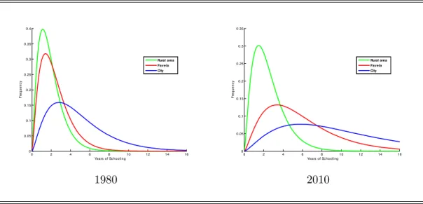
Brazil, as many developing countries around the world, experienced a fast process of structural transformation and urbanization after World War II. Given housing prices, many rural -urban migrants could not a§ord to buy a spot in the cities and had to live in slums, that grew very fast in the period and do not seem to be reducing in size. Living in cities entails better work opportunities, even for those in slums, higher income and better education. For the residents of the favelas the expected schooling of their children, controlling for the education of the parents, is

9_{See www.ibge.gov.br/english/.}

10_{The UN Habitat defines a slum household as a group of individuals living under the same roof and lacking one or}

more of the following conditions: (i) Access to improved water;(ii) Access to improved sanitation; (iii) Su¢cient-living area; (iv) Durability of housing; (v) Security of tenure.

11_{For more details see www.emop.rj.gov.br/trabalho-tecnico-social/censos-comunitarios.} 12_{National Household Survey conducted every year in Brazil since 1976.}

above the education of the children of the rural dwellers but smaller than the education of the city kids who live outside slums. Slum residents work mostly on low skill services and manufactures (in this case, construction), while non-slum urban workers are more evenly distributed among high and low skill services and manufacture. This section documents these facts.

In sixty years, Brazil went from a predominantly agricultural and rural economy to an urban economy with the services sector playing a dominant role. From Figure 1, we see that the share of

labor employed in agriculture13 _{decreased steadily from 64% in 1950 to 16% in 2010, at the same}

time that urban and slum populations increased.

Figure 1: Value Added per Sector, Population in Slums 19500 1960 1970 1980 1990 2000 2010 6 12 18 24 30 36 Va lu e -A d d e d p e r W o rk e r Year 1950 1960 1970 1980 1990 2000 20100 0.1 0.2 0.3 0.4 0.5 0.6 0.7 0.8 0.9 1 Sh a re o f Po p u la ti o n

Workers outside agriculture Pop. in urban locations Pop. in slums, Rio de Janeiro Agric. productivity Non-Agric. productivity

Regarding the evolution of productivity14 _{(output per worker) agriculture presents a clear}

up-ward trend between 1950 and 2010 at the same time that one observes a rise followed by a fall in the non-agriculture productivity. For the period 1950-1980, the productivity in this sector grew by 2% per year, as well as in agriculture. The outstanding reallocation of labor from agriculture to non-agriculture (much more productive) during this period resulted in a convergence in direction

to the U.S. economy and an acceleration of Brazilian aggregate productivity15. But in 1980 the

picture changed. Since this year, non-agriculture productivity has fallen 1% per year. After the labor reallocation from lower to higher productive sectors, the next step would be to invest in hu-man capital and give better opportunities to those rural-urban migrants and their o§spring. That did not happen, and a very large uneducated workforce had to work in low skill sectors with poor growth prospects.

Since the early twentieth century, we observe waves of rural-urban migration and the emergence of the first slums in Rio de Janeiro (capital of Brazil during the years 1763 to 1960), but it was only

13_{The series of real value-added and employment by sectors were taken from the Groningen Growth and}

Develop-ment Centre (GGDC) database (see Timmers et al. 2014).

The ten broad sectors of the dataset were grouped here into two major sectors: agriculture, consisting of agriculture, forestry and fishing; and non-agriculture, which is composed by the remaining sectors.

14_{Productivity was constructed as the ratio between the real value added and the persons employed by each sector}

for the period 1950 to 2010.

15_{Silva and Ferreira (2011) finds that 45% of the 1950-1980 growth in Brazil is due to structural transformation}

after World War II that the process of urbanization and formation of slums became a national and widespread phenomenon. Pearlman (2010) notes that, before World War II, only 15% of Brazilians lived in cities. According to Census data, the urbanization rate was already 36% in 1950 and in the next thirty years a very large change in the rural-urban distribution of the population occurred. By the mid 1960s there were already more people living in cities than in the country-side: the urban population went from fewer than 13 million in 1940 to more than 50 million in 1970. By 2010 only 15% of the Brazilian population lived in rural areas.

Rural-urban migration is the most important force driving the urbanization process in developing

countries16_{. World Bank (2008) estimates that around 40 million people left the countryside or poor}

regions for larger cities between the years 1960 and 1970, period of high economic growth in Brazil. This process continued in the following years. In 1960, as shown in Table 1, 40% of the people living in Rio de Janeiro were migrants, and this should be true for most large cities in the country. Although this process slowed down after the seventies, there were still 1.5 million migrants living in Rio de Janeiro in 2000, approximately 27% of its population.

Table 1: Migrants, (% of total population) Rio de Janeiro

Year Slums City

1960 52.2 38.3

1991 29.8 27.7

2000 31.2 25.8

Source: Brazilian Census

The rural-urban migration resulted in a fast expansion of slums - a widespread reality across large cities - and the agglomeration of low skill labor in manufacturing and mainly in services sectors. From Table 1 we can see that in 1960 more than half the residents of slums in Rio de

Janeiro were migrants17_{. São Paulo and Rio de Janeiro are the two richest cities in Brazil (in terms}

of GDP) and have some of largest shares of population living in slums, as shown in Table 2: Table 2: Urban population living in slums (%)

Cities

Year Rio de Janeiro São Paulo Belo Horizonte Belém Salvador

1950 7.0 — — — — 1960 10.2 — — — — 1970 13.3 — — — — 1991 17.4 9.2 14.2 25.8 10.1 2000 18.5 11.1 12.3 34.6 9.6 2010 22.0 23.2 — — —

Source: Brazilian Census

Rio de Janeiro is the only city for which we have information about urban and slum populations since 1940. The share of the Rio de Janeiro population living in slums went from 7% in 1950 to 22% in 2010. In São Paulo in 2010, 23% of total population was living in slums, more than doubling in twenty years. There were 2.1 and 1.7 million people living in slums in the metropolitan regions of São Paulo and Rio de Janeiro, respectively, in 2010. Thus, the slum phenomenon appears to be a reality that expands every year and is not a transitory phase.

16_{For more details about urbanization and rural-urban migration in developing countries, see Brueckner and Lall}

(2015) and Lall et al. (2006).

17_{It is also true, according to the 1991 Census, that the share of migrants coming from rural areas is two times}

Rural-urban migration depends on forces known in the literature as pull and push. The forces that pull migrants to their destinations are better economic opportunities in terms of jobs (due to agglomeration economies) and better amenities and public services such as piped water, electricity, hospitals and schools. And the forces which push migrants o§ their origin lands are low productivity in agriculture, environmental changes, pressures of population growth and lack of access to basic public services. Lall et al. (2009) study migration from lagging to leading regions in Brazil and the pull and push forces. They find that wage di§erences are the main factor driving migration. Access to basic public services matters a lot, they show that poor people are willing to accept lower wages in order to get access to better amenities and quantify how much is this willingness to pay for three public services (hospital, water access and electricity). Along the same lines, Dudwick et al. (2011) investigate why migrants are attracted to particular locations in Nepal. They show that destinations with better access to schools, hospitals and markets are the most preferred ones.

Here, we are interested in studying and focusing on two main pull forces: better economic

opportunities and access to better education18_{. In the first case, migrants are looking for better}

jobs and higher income. In Table 3, we see that the total income of people living in urban areas, controlling by education, is significantly higher than of those who live in rural areas.

Table 3: Income Ratios by Education and Location (2000)

Brazil Rio de Janeiro São Paulo

Education Urban/Rural City/Rural Slum/Rural City/Rural Slum/Rural

Average 2.5 4.2 1.3 4.5 1.4 0 1.3 2.1 1.6 2.5 2.0 1 to 3 1.4 1.9 1.4 2.1 1.6 4 1.3 1.6 1.1 1.8 1.2 5 to 8 1.3 1.6 1.0 1.7 1.0 9 to 11 1.4 1.6 0.8 1.8 0.9 12 or + 1.3 1.4 0.5 1.5 0.5

Source: Brazilian Census

On average, income in urban area is two and a half times larger than in rural areas, and this is also true for all years we have data (1970 to 2010). And that is not only due to a composite e§ect (there are less educated people in rural areas), but also due to the fact that at every education level mean income in the cities is higher than in the countryside. For those with four years or less of education, for instance, average income in 2000 in the rural region was only 74% of average income

in the cities19.

Even when rural migrants move to cities and end up living in slums, their expected income is still higher than those who stayed in the rural areas, specially in the case of the less educated (the vast majority of rural and slum residents), as we can see from the figures in Table 3. While a typical resident in the slums in Rio or São Paulo makes less than someone with the same educational level living outside the slums, he makes considerably more than a corresponding person who lives in the

countryside of Brazil20_.

18_{We are not saying that the other pull and push forces are not relevant, but following the literature that}

re-lates growth and human capital, we are interested in investigates how structural transformation, urbanization and education can explain the stages of economic growth.

19_{Ferreira, Menezes and Santos (2005) find that there is positive selection of migrants in Brazil, and this can}

partially explain the income di§erence between rural and urban areas. However, they estimated that this can only explain 10% of the income disparity, which is only a fraction of the numbers in Table 3. Other forces are contributing for the bulk of the income di§erence.

20_{This is also true for most large cities in Brazil, with the exception of Salvador, where incomes are about the}

People migrate to cities, among other reasons, to have access to better jobs, even if they live in slums. From Table 4 we can see that the slums residents work mostly in cities (out of the slums), where the majority of opportunities and jobs are. And this is true even though they earn less than the cities residents, as we saw in Table 3.

Table 4: Job location of people living in three slums in Rio (%)

Alemão Manguinhos Rocinha Mean

Inside slums 22.70% 22.40% 22.00% 22.40%

In the close vicinity 15.70% 19.30% 6.90% 13.90%

Outside slums 61.60% 58.40% 71.10% 63.70%

Source: Favela Census of Rio de Janeiro

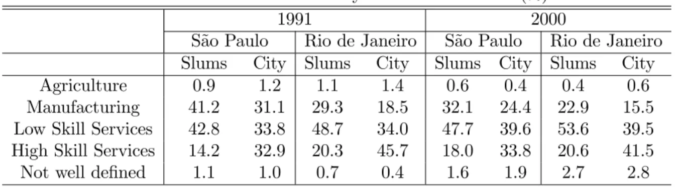
What are the sectors in which slum residents work, and are they very di§erent from the sectors in which non-slum residents work? Data from the 1991 and 2000 Census (see Table 5) show some similarities and important di§erences. As one could expect from their lower education levels, slum residents are distributed more heavily across low skill sectors. In São Paulo and Rio, in 2000, around 50% of workers living in slums are in the "Low Skill Services" sector, which is mostly personal services (e.g., maids), retail and restaurants. The corresponding figures for non-slum residents are considerably smaller. There are proportionally fewer high skill workers living in the slums (and half of them are in the "Transportation, Storage and Communication" sector, which is partially a low skill sector). In contrast, the share of workers in the high skill sector living in the city is, in general, twice as large as those in the slums, and the concentration in the Health, Education,Government

and Financial Services sub-sectors is much larger21.The proportion of workers in manufacturing is

larger in slums, but this is mostly due to the construction22 _subsector.

Table 5: Labor distribution by sector and location (%)

1991 2000

São Paulo Rio de Janeiro São Paulo Rio de Janeiro

Slums City Slums City Slums City Slums City

Agriculture 0.9 1.2 1.1 1.4 0.6 0.4 0.4 0.6

Manufacturing 41.2 31.1 29.3 18.5 32.1 24.4 22.9 15.5

Low Skill Services 42.8 33.8 48.7 34.0 47.7 39.6 53.6 39.5

High Skill Services 14.2 32.9 20.3 45.7 18.0 33.8 20.6 41.5

Not well defined 1.1 1.0 0.7 0.4 1.6 1.9 2.7 2.8

Source: Brazilian Census

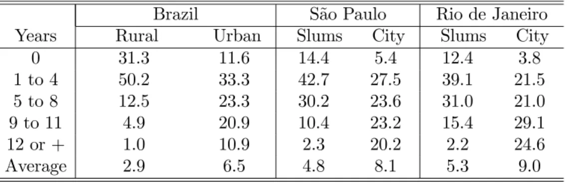
Migrants also move to the cities looking for access to better education, because higher levels of education mean higher income on average and also because they care about their children’s future. Average education is much lower in rural than in urban areas, as shown in Table 6. The mass of population in the first two levels of education is much higher in the countryside than in urban areas

and the average years of schooling is much lower for all years we have data (1970 to 2000)23_.

21_{As for the labor distribution by sector in the rural area, between 87% and 71% of the workers are in the agriculture}

sector, depending on the Census year. In contrast, only 6% of urban residents worked in the agriculture in 2000.

22_{Without construction subsector, 17% of the labor force in São Paulo and around 10% in Rio de Janeiro worked}

in manufacturing in 2000.

23_{In 1970, average schooling in the countryside was less than one year and 64% of the adult population had no}

Table 6: Population distribution by years of schooling, 2000 (%)

Brazil São Paulo Rio de Janeiro

Years Rural Urban Slums City Slums City

0 31.3 11.6 14.4 5.4 12.4 3.8 1 to 4 50.2 33.3 42.7 27.5 39.1 21.5 5 to 8 12.5 23.3 30.2 23.6 31.0 21.0 9 to 11 4.9 20.9 10.4 23.2 15.4 29.1 12 or + 1.0 10.9 2.3 20.2 2.2 24.6 Average 2.9 6.5 4.8 8.1 5.3 9.0

Source: Brazilian Census

As one could expect, average education of slum residents is lower than of those living in formal cities. From Table 6 we can see that in Rio de Janeiro in 2000 the average adult education in the slum was almost 4 years smaller than in the city, and similar figures are true for São Paulo (and 1991). However, education levels in the slums of Rio and São Paulo are well above those in the rural areas of Brazil. On average, a slum resident of Rio de Janeiro in 2000 had two and a half years of schooling more than a typical resident of the rural areas. And while one third of the rural area residents in this same year had no education at all, only 12% of the slum residents of Rio had no education. Clearly, rural area populations are less educated than those in slums that are, in their turn, less educated than city dwellers.

Upward mobility is very pronounced in cities, specially for those with few years of schooling, when compared to rural areas. From PNAD 1996 supplement we can show that average years of schooling of a person whose parent had no education was almost two years smaller in the rural areas than in urban areas (2.65 and 4.48 years, respectively), and similar figures are obtained for those with parents with 1 to 4 years of education. Upward mobility is higher in formal cities than in slums, but for all metropolitan areas (that we have data) it is still higher in slums than in rural areas. For instance, in Rio de Janeiro and São Paulo the average schooling of someone whose father has no education was, in 1996, 5.58 and 3.94, respectively, way above the corresponding figure for rural areas we just saw. For the formal city, the values are even higher: 9.91 and 9.23, respectively. These numbers indicates that education mobility is higher outside than inside slums, and higher in slums than in the rural areas.

Another important evidence on di§erent intergenerational mobility comes from transition

matri-ces of individual education conditional on their parents education24_{. Figures 2a and 2b, constructed}

from transition matrices estimated using 1988 PNAD data for the Rio de Janeiro, show the likeli-hood of schooling attainment for rural, urban, slum and outside slum areas of children with parents

with no education at all and with one to four years of schooling, respectively25_.

24_{See Ferreira and Veloso (2003) for Brazil in 1996.}

25_{We assume that the households living in metropolitan areas with total income in the 35 percentile or lower are}

Figure 2a: Education of a children with father with no schooling

Figure 2b: Education of a children with father with 1-4 years of schooling

There is a great persistence of low educational levels in rural areas and upward mobility in urban areas. For example, in 1988, 52.08% of parents in the countryside with no schooling had children with the same level of education, compared with half this figure (27.58%) in cities. Similar results are found for the children with parents with 1 to 4 years of education: around 70% of them will have the same level or less education than their fathers, as opposed to less than 40% in the case of urban children. And in urban areas, 62.8% of parents with 12 or more years of schooling have children with the same level of education, while in rural areas the corresponding figure is only 30.6%.

The numbers in the transition matrices for slums are better than those for rural areas and worse than those for non-slum areas. In slums, 35% of parents with no education had children with no education too, 17 percentage points below rural areas in Brazil. The corresponding figure for city residents in Rio de Janeiro is only 16%. In the city 64% of parents with 12 or more years of schooling had children with the same level, but in the slum this was only 28%, although there were very few observations in this case. Thus, the persistence of low levels of education in slums is smaller than in the countryside but the upward mobility is worse than in the cities. Therefore, leaving the countryside is a first step to get better living conditions, but living in slums is not a good option compared to cities. The next step is to move away from slums.

Schools in slums are, in general, worse than in the formal cities as tests and quality of education measures tend to confirm. While parents benefit from jobs outside slums, education, in contrast, is mostly done inside the slums, or in their close vicinity. From Table 7 one can see that around three quarters of the students in these three slums attend schools inside the favela or less than 3 kilometers away. This may partly explain lower upward education mobility in slums.

Table 7: Percentage of students by location of school (living in these 3 slums)

Alemão Manguinhos Rocinha Mean

Inside slums 86.30% 55.90% 43.30% 61.80%

Outside but <1km away 8.90% 21.30% 0.50% 10.20%

Outside between 1-3km way 0.00% 12.30% 26.00% 12.80%

Outside >3km 1.50% 7.80% 30.20% 13.20%

Could not locate school 3.30% 2.70% 0.00% 2.00%

Source: Favela Census of Rio de Janeiro

One last important stylized fact is the di§erence of housing costs across locations. As shown in Table 8, rent prices in urban areas of Brazil was in 1991 more than twice as expensive than in rural areas on average, and renting 3 bedroom apartments was three times as expensive as in the countryside. Rents in the slums of Rio de Janeiro and São Paulo were also considerably more expensive than in the countryside of Brazil and this should be true everywhere, as slums are mostly located in large cities. But as expected, prices in formal cities are well above those in slums; in the

case of Rio and São Paulo around twice as much on average. The di§erence of rent prices between non-slums parts of these two cities and the rural areas of Brazil, is huge, more than four times on average in the case of São Paulo. Hence, living in the rural areas is considerably cheaper than living in the slums of Rio and São Paulo which are, in its turn, less expensive than living in non-slum parts of the city.

Table 8: Ratio of Monthly Rents (1991)

Brazil Rio de Janeiro São Paulo

# Bedrooms Urb./Rur. City/Rural City/Slum City/Rural City/Slum

1 2.0 3.2 1.8 3.5 1.5

2 2.3 3.5 1.9 4.7 2.0

3 2.9 4.8 2.7 6.5 2.6

Average 2.3 3.6 2.3 4.1 1.9

Source: Brazilian Census

4

Model

We consider a simple model that can be used to analytically examine: (i) structural transformation; (ii) urban development; (iii) income and skill distribution; (iv) social mobility. Our attention is focused on the allocation of individuals —and their skills— across locations, production sectors and occupations and on the dynamic implications of those decisions for the skill formation of future generations. We first lay out the environment and then define a competitive equilibrium. In the next section, we examine the equilibrium allocations, providing a number of simple but key analytical results on the emergence and persistence of slums.

4.1

The Environment

We consider a discrete-time, infinite-horizon economy populated by dynasties of two-period-lived overlapping generations (OLG) of individuals. Time periods are indexed by t = 1, 2, 3, ... In any period, individuals di§er in their skills. The population of the economy, whose size is normalized to

one, is described by a probability measure µ_{t defined over all positive levels of skills z 2 R}+. The

evolution over time of the distribution of skills, {µt}1t=1 is determined endogenously, as part of the

equilibrium of the economy, since adults of any period t draw skill levels from distributions a§ected by the decisions of their parents as explained below.

Adults choose occupations, locations and the consumption of goods. In this model economy, there are three locations: rural areas, slums (favelas) and city, which we index by l = R, F , C, respectively; there are two production sectors, agriculture and non-agriculture (manufacturing and services), which we index by i = A, N ; and, there are three occupations or types of labor services: unskilled, qualified and adaptable labor. We index these types of jobs as j = u, q, a, respectively.

Preferences: The utility of a households at time t is defined over the consumption of goods and over the expected well-being of their children. Specifically, the utility of an adult at t is given by:

Vt= u(ct) + βEt[zt+1],

where u(·) is the individual’s utility over consumption. Here, the consumption vector, ct =

!

cA

t, cMt

" , consists of consumption levels of agricultural and non-agricultural goods, respectively. As a driver of structural transformation, we assume the standard Stone-Geary non-homothetic preferences:

u (ct) =!cA_{t − ¯c}A"αA!

cN_t "1−αA

where 0 < αA< 0 is a share parameter and cA > 0 is a minimum consumption floor of agricultural goods (food.)

For tractability, we assume a form of impure altruistm, i.e. paternalistic preferences (à la Fernandez and Rogerson, 1998) where parents care about the expected skills of children. Here,

β > 0 indicates how much weight parents put on their childrens expected skills for the next period,

zt+1, and Et(_{·) is the (correct) expectation of those skills given the information available at the}

time.

Supply of Skills: All workers can in principle provide three di§erent types of labor services.

First, regardless of how low or high their skills z are, everyone can provide one unit of unskilled

labor. Second, those workers with skills above a minimum qualification requirement, zmin > 0, can

supply one unit of qualified labor; those below that threshold have zero supply of those skills. Third, all individuals can supply adaptable labor services in proportion to their skills. More formally, the occupation choices, a given by the mutually exclusive options to provide labor skills as follows:

unskilled : hu(z) = 1 _{for all z 2 R}+;

qualified : hq(z) =

#

0 if z < zmin,

1 otherwise;

adaptable: ha(z) = z _{for all z 2 R}+.

Production of Goods: For simplicity, we abstract from agricultural goods production in the city and from non-agricultural goods production in the rural areas. Therefore, for production, we only

need to specify the agricultural productivity XA

t in rural areas and non-agricultural productivity

XN

t in urban areas.26 We assume that both consumption goods are produced using only labor.

Specifically, the country’s aggregate output of production of agricultural goods, YA

t , is just given

by

Y_tA= X_tALu_t, (1)

where Lu

t is the aggregate units of rural labor, which, in our simple model is entirely unskilled.

services. On the other hand, production of non-agricultural goods requires both, qualified and adaptable labor, i.e.

Y_tN = X_tN (Lq_t)η(La_t)1−η, (2)

where 0 ≤ η ≤ 1 is a share parameter. Here, Lqt and Lat are, respectively, aggregate supply of

qualified and adaptable labor, which, by assumption, are located in urban areas, as explained below.

Both, agricultural and non-agricultural goods are fully tradable within the three regions of the country.

Locations: Occupations and Housing Costs. Households decide whether to live in a rural or urban area, knowing the implications of those decisions for housing costs of occupation opportunities. In our simple model, the provision of unskilled labor is the only occupation available for households living in rural areas. For households living in urban areas —cities and slums— their occupation choices are between providing adaptable or qualified labor, the latter subject to the qualification requirement.

Housing costs di§er across the three locations. For our purposes, housing costs di§erences matter because (a) higher urban housing costs serve as a barrier to structural transformation, and

26_{In principle, the three locations l in the country have (exogenous) productivities across sectors i described}

by an arraynX_tl,io of positive numbers. While extending the model along this dimension is straightforward, the entanglement of carrying additional variables more than o§sets the gains in realism, given the small shares of agricultural production in urban areas.

(b) higher housing costs in cities serve as a barrier to the acquisition of skills for children living in slums. The simplets way to capture both of these forces is as follows: First, as a normalization, we assume that living in the rural area entails no direct housing costs. Second, living in the city entails a fixed cost, paying for one unit of housing. For simplicity, we assume that housing do not deliver utility directly, and simply gives access to living in the city. Constructing a house requires

ξ_t = "0(σt)"1

units of non-agriculture goods, where "0, "1 are positive parameters and σt is the size of the city,

i.e. the total mass households living in it. Hence, as described in the equilibrium section, housing

prices ph

t, are endogenously determined by the structural transformation of the country, both, by

of the relative price of non-agricultural goods and by the size of the city.

Finally, we assume that living in a slum entails no direct housing costs. Instead, it entails other costs, such as time commuting and time and goods committed or lost because of crime and lack of property rights and protections. To capture those costs, we assume that households living in a slum lose a fraction τ of their consumption of goods. While stark, these modeling choices parsimonious and transparently delineate the housing costs vs labor and occupation choices of urban-rural migration as well as the schooling choices as explained next.

Locations and Production of Skills. At any time t, the adult population in the economy is

described by a probability distribution µt(·) of skill levels z, with support over all the positive

reals, [0, 1). From the location decisions of each household, each location l ends up being with a

subpopulation µl

t(·), i.e.,

µ_t(_{·) =} X

l=R,F,C

µl_t(_·).

Location decisions determine the formation of skills for the children growing up in each location. We model this as follows: Let

Z_tl _≡ 'R1 0 z ρ_µl t(dz) R1 0 µ l t(dz) )1/ρ ,

be the average skills of the adults living in location l = R, F, C. Here, ρ is a parameter determines the curvature in this average and will determine the behavior of human capital externalities and the

persistence and mobility of skill levels across generations. In any event, Zl

t determines the exposure

to ideas of each children in each location. We assume that each child draws a skill level from a

distribution Q (·) that is shifted by Zl

t, i.e.,

z0 _{∼ Q}!_·|Ztl".

We assume that Q!_·|Ztl

"

has a continuous density with full support in the non-negative reals [0, 1),

and that Q (·|·) is increasing in the sense that for any Z1 > Z0, then Q (·|Z1)dominates Q (·|Z0)in

the first order sense. In particular, in our numerical implementation of the model, we will assume

that Q!_·|Zl

t "

is a Gamma distribution with mean Zl

t.

For the country as a whole, in the next period, the population of adults µ_t+1(_{·), will be composed}

by the children that grew up in all three regions in the previous period, i.e.

µ_t+1(_{·) =} X l2{R,F,C} Z ₁ 0 Q!B _{| Zt}l"µl_t(dz).27

4.2

Equilibrium

We now define competitive equilibria of this environment. First, the state variable of the country

is given by St = !µ_t, XtA, XtN

"

sectoral productivities. Using agricultural goods as a numeraire, the price systems is composed

by price of non-agricultural goods pN

t , the unitary prices of unskilled, qualified and adaptable

labor skills, +wl_t, w_tb, wa_t,, and housing prices in the city, ph

t. Given those prices, in all periods

t, households of all skills z decide their consumption ct(z) = +cA

t (z), cNt (z) , , their occupation, + χl t(z), χ q t(z), χat (z) , , and of location,+χR t (z), χFt (z), χCt (z) , .

We now lay out the conditions for a competitive equilibrium. We first consider production. The two goods are produced in competitive markets. Firms take goods prices and wages as given and maximize profits. Agricultural goods producing firms hire unskilled labor to maximize:

max

Lu

t

+

pA_t Y_tA_{− w}l_tLu_t,.

Since agriculture is our numeraire (pAt = 1), and YtA = XtALut, then the equilibrium wages for

unskilled workers are simply

w_tl = X_tA. (3)

Non-agricultural goods producing firms hire qualified and adaptable labor to maximize: max

Lqt, Lat

+

pN_t Y_tN _{− w}q_tLq_{t − wt}aLa_t,,

subject, respectively, to the production function (1) or (2).

Since YN t = XtN(L q t) η (La

t)1−η, the equilibrium wage conditions have a very familiar forms in

terms wq_t = ηpN_t X_tN -La t Lq_t .1−η . (4) wa_t = (1_{− η) p}N_t X_tN -Lq_t La t .η . (5)

Consumption of Goods: Consider a household with income yt, he chooses the consumption

of goods to solve: / cA_t , cM_t 0 = arg max Q i2{A,M} ! ci_{t− c}i"αi s.t. P i2{A,M} pi_tci_{t≤ y}t.

The optimal consumption levels are given by:

ci_t= ci+ αi pi t " yt− P i2{A,M} pi_tci # .

This implies that the intra-period indirect utility of someone with income yt and facing prices

{pi

t}_i2{A,M} is given by:

vt(yt) = Q i2{A,M} " αi pi t yt− P i2{A,M} pi_tci !#αi .

Occupation Choices: Conditional on the location decision, the household choose his

occupa-tion maximizing the income coming from labor supply. Thus, given his skill z and current wages

wl,j_t , wtb,j and w

a,j

t , the income e

j

t(z) can be simply written by:

ej_t(z) = maxnw_tl,jhl(z), wtb,jhb(z), w

a,j

t ha(z)

o .

Location Choices: Given prices+pi,j_t ,, optimal conditional occupation choice ojt(·) and optimal

conditional income ejt(·), the expected discounted utility of a household with skill z at time t is

defined by: Vt(z) = max j2{R,F,C} Q i2{A,M} " αi pi,j_t y j t(z)− P i2{A,M,S} pi,j_t ci !#αi + βEt/zt+1|Ztj 0 , where: y_tj(z) = 8 < : eR t(z) if j = R; (1_{− τ ) e}Ft (z) if j = F ; eC t (z)− pht if j = C;

is the income net of housing costs (income cost τ in slums and monetary cost ph

t in cities).

Therefore, the optimal location decision is the solution of:

j_t∗(z)_{2 arg max} j2{R,F,C}vt ! y_tj(z)"+ βEt/zt+1|Ztj 0 .

Given the country’s probability measure of skills µt(·), the assignment (selection) of workers into

regions defines the measure of skills µjt(·) for region j at time t as:

µj_t(B) = Z B χ_{z:j∗ t(z)=j}(z) µt(dz) where χ_{z:j∗

t(z)=j}(·) is an indicator function that takes a value equals to 1 if individuals of skills z

are assigned into region j and zero otherwise; B is any Borel set on non-negative real numbers.

4.2.1 Definition of Equilibrium

Given the above definitions, we can write the following aggregates:

1. Production: The output levels of agriculture and non-agriculture goods are:

Y_tA= Y_tA,R= AA_tLl,A,R_t ,

and

Y_tM = YtM,U = AMt

:

Lb,M,U_t ;η:La,M,U_t ;1−η.

2. Regional and country’s aggregate incomes:

Y_tj _≡ Z y_tj(z) µjt(dz), and Yt ≡ X j2{R,F,C} Z y_tj(z) µjt(dz).

3. Aggregate Consumption (of each good):

C_ti _≡ Z ci_t(yt(z)) µ_t(dz) = ci+αi pi t 2 4Yt− X i2{A,M,S} pi_tci 3 5 ;

4. Labor supply of low, amenable and basic skilled labor: Ll_t = Z Ml,Rt µ_t(dz), La,U_t = Z Ma,Ft µ_t(dz) + Z Ma,Ct µ_t(dz), Lb,U_t = Z Mb,Ft µ_t(dz) + Z Mb,Ct µ_t(dz).

where Mo,jt is the set of individuals who work at occupation o at location j.

With all above definitions in mind, now we can define the equilibrium of this model.

Definition Given an exogenous sequence of aggregate productivities +Ai,j_t , and an initial skill

distribution µ0(·), an equilibrium will be composed of:

1. Individual location j∗

t(z), occupation o

j

t(z) and demand decisions c

i,j

t (z) for each period and

skill level z.

2. An endogenous sequence of probability distribution measures {µt(_·)}1_t=0 for the skills of the

country;

3. Sequences +µj_t(_·),1_t=0 of non-negative measures describing for each t how location choices

allocate µ_t(_{·) across locations j.}

4. Sequences of aggregate outputs Yti,j and consumptions C

i,j

t ;

5. A sequence of prices +pi,j_t , for the goods i in locations j at time t.

Such that:

1. Individual optimization: Given prices +pi,j_t ,, decisions +j_t∗(z), ojt(z), c

i,j

t (z)

,

are optimal.

2. Adding up: For any t and for any Borel set B ⊂ R+

µ_t(B) =X

j

µj_t(B) .

3. Aggregation Consistency: For all t, given the pre-determined µt(·), for all locations j:

µj_t(B) =

Z B

j_t∗(z)µt(dz) for any Borel set B.

4. Market-Clearing conditions: • Goods markets (both tradeable):

X j2{R,F,C} C_tA,j = Y_tA; X j2{R,F,C} C_tM,j = Y_tM.

• Labor markets:

Rural : Ll,A,R_t = Ll,Rt ,

Urban : La,M,U_t = La,U_t , and Lb,M,U_t = Lb,U_t .

5. Law of Motion of Demography and Skills: The country’s population evolves according to: µ_t+1(B) =X j Z Qt ! B _{| Zt}j"µj_t(dz),

for any Borel set B ⊂ R+.

In the next section, we derive some simple analytics on the conditions under which slums arise in equilibrium.

5

Equilibrium Allocations

We first provide a simple result on the occupation choices, conditional of location choices. The result is useful for describing equilibria in a number of contexts. We then use the result to explore the properties of the equilibrium location choices.

It can be easily shown that the equilibrium of this economy can be characterized by location

and occupation thresholds. For locations, the support of µt, the population of skills in the country

will be divided according to two thresholds 0 < zR

t ≤ zFt < 1, defining three groups: (a) rural

population, µ_t/0, zR t 0 , (b) slum population, µ_t!zR t , ztF 0

and (c) city population µ_t!zF

t ,1

"

. For short,

we will call those in (b) and (c) as the urban population µt

!

zR

t ,1

" .

For occupations, in our highly simplified model, there is only the choice of urban dwellers of

o§ering qualified or amenable labor. To that end, we only need to define the threshold ztH ≥

max+zR

t , zmin

,

, so that the supply of basic qualified labor is µ_t/max+zR

t , zmin

,

, zH

t 0

and the rest of the urban population would be employed in amenable jobs. For future reference we will call an

allocation to be with urban low skill services jobs when zR _{< zmin, i.e. when some urban}

dwellers do not qualify to provide basic skilled labor. Similarly, we say that an allocation is high

skill urban jobs only when zR _{> zmin. In the first case, the marginal migrant from the country}

side enters the urban locations to work in low skill services. In the second case, the marginal worker would enter to work in qualified occupations and all the amenable service sector jobs will be provided by individuals who could have performed qualified jobs.

We now explore the behavior of these thresholds in our model economy, starting with the simplest cases and progressing towards the general model.

5.1

Conditional Occupation Choices

Conditional on any urban-rural divide, zR

t , the equilibrium occupation choice ztH can be readily

solved from the maximization of non-agricultural output YM_{. Denoting Ft the c.d.f. associated}

with µt, the aggregate supply of both forms of labor services can be written entirely in terms of the

thresholds zR _{and z}H_: Lb = Ft!zH"_{− F}t ! max+zR, zmin," and La = Z max{zR_{, z} min} zR zµ_t(dz) + Z 1 zH zf (z) dz.

Then, the occupation divide zH within the urban area can be simply writen as: max zH Y M!_zH_{; z}R"_{= Z}M/_F !_zH" − F (zmin)0η "Z max{zR_{, z} min} zR zµ_t(dz) + Z 1 zH zf (z) dz #1−η . The first order condition of this maximization implies that the solution is the fixed-point implied by the following equation:

zH = η 1_{− η} ∗ '_R max{zR, zmin} zR zµt(dz) + R1 zHzµt(dz) ) [Ft(zH_{)− F} t(max{zR, zmin})] . (6)

While closed-form solutions for the optimal occupation split, zH!_zR"_{, and for the resulting}

output of non-agricultural goods, YN!zR", cannot be provided, we can prove the following

charac-terization:

Proposition 1 Given a population µt and a rural-urban divide, zR > 0, there exists a unique

occupation threshold zH _<

1. If the measure µt is continuous and with unbounded support, the

threshold zH _{is continuous. If (i) z}R _{< zmin, then z}H _{is locally strictly decreasing in z}R_{, but if}

(ii) zR _{> zmin, then z}H _{is locally strictly increasing in z}R_{. Optimized non-agricultural output,}

YM!zR"_{≡ max}zHYM

!

zH; zR" is always strictly decreasing in zR.

This simple proposition, whose proof is deferred to Appendix B, characterizes the occupation decisions inside a city. The most interesting aspect of this proposition is the non-monotonicity of the occupation threshold in terms of the size of the city. In particular, given the population

distribution of skills µt, if the city grows (i.e. a lower zR when initially zR< zmin), and this growth

expands the supply of low-skill amenable labor, then the high-skill amenable sector becomes more

selective (higher zH.) An obvious implication is that the expansion of the city in this case would

lead to more income inequality across its dwellers. On the other hand, if the city expansion (i.e.

a lower zR when initially zR > zmin), then the distribution of income inside the city becomes less

disperse, as the high-skill sector becomes less selective (lower zH_{) in order to expand.}

The implication that YM!_zR" _{is decreasing in z}R _{is straightforward.}

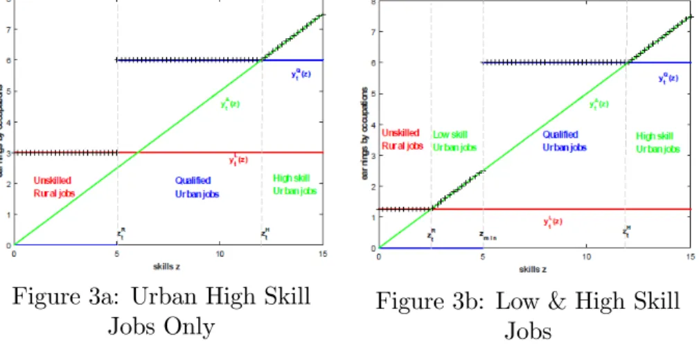
Figure 3 displays these two occupation configurations. In panel 3a, zR _{> z}

min so that there are

no low skill amenable jobs in the economy, just high skill jobs. In panel 3b zR _{< zmin, there are}

now low and high skill amenable jobs in the economy.

Figure 3a: Urban High Skill Jobs Only

Figure 3b: Low & High Skill Jobs

5.2

Location Decisions

We now explore the location decisions. For exposition clarity, we do this exploration, starting with the simplest case of a static economy, and progressing to the more general specification of our model.

5.2.1 Equilibria in Static Economies

We first consider a case with myopic allocations, i.e. β = 0, when individuals are allocated across regions and occupations without considering the implications for their children’s skill accumulation. We then examine the model when location decisions are also based on the skill formation of children. To isolate the role of housing as a barrier to entry in the city, we first consider the case when housing is not an issue.

No Housing Costs, ph

t = 0 We begin with the case in which ξ = 0, i.e. housing costs are

negligible in the city. Obviously, slums would be empty, as they would be unnecessarily costly for

anyone to opt for living there. In terms of our thresholds, this implies zF

t = zRt . Here, the only

location decision is the traditional rural-urban divide zR

t . To solve for equilibrium locations, we

need to solve for the prices of the goods produced in the di§erent locations.

We use the price of agricultural goods as the numeraire, pA _{= 1. Given, their income, individual}

household will maximize their utility. It is straightforward to show, that the optimal consumption

levels !cA_{, c}M" _{for all consumers satisfy}

pM = (1− αA) αA -cA t − ¯cA cM . . (7)

It is straightforward to see that this condition carries over to the aggregate levels CtA and CtM.

Hence with CA t = YtA ! zR"_{= X}A t Ft(zR) and CtM = YM(zR), we obtain pM_t !zR"= (1− αA) αA " XA t Ft ! zR t " − ¯cA YM t (ztR) # . (8)

Notice that the price of non-agricultural goods, pM

t !

zR" _{is strictly increasing in z}R _{(when the}

urban areas shrink). Moreover, the price of non-agricultural goods goes to zero if the rural areas

becomes too small, i.e. zR

t approaches Ft−1 h ¯ cA ZA t i . Lastly, pM t ! zR"

goes to +1 when the city

completely over disappears, i.e. if zR_{! +1. These simple properties of the price p}Mt

!

zR" will be

useful to establish the equilibrium location decisions.

For brevity, we will define θ/pM0 _{≡ [α}A]αAh1−αA

pM

i1−αA

, a simple function that will be used to describe the utility levels of the di§erent households in the di§erent location options.

According to their skills z, the welfare of the households in each location is:

• Rural Area: The only option available is to work in agriculture, o§ering low skill services.

Having normalized pAt = 1, the income of everyone is simply ZtA in units of agriculture goods.

The attained utility of everyone in the country-side is:

VR!zR" = θ/pM_t !zR"0 /X_tA_{− ¯c}A0. (9)

It is independent of the individual’s skill level and strictly decreasing in zR_{, as smaller cities}

• Urban Area: The attained utility of the households livings in cities depends both, on their occupation and skills levels. Unitary wage rates for amenable and basic qualified labor services are given by wa_t !zR"= (1_{− η) p}Mt ! zR"X_tM L b t ! zR" La t (zR) !η ; wtb ! zR"= ηpMt ! zR"X_tM L a t ! zR" Lb t(zR) !1−η , (10)

where the aggregate labor supplies are defined as Lb!_zR"_{= Ft}/_zH!_zR"0

−Ft ! max+zR_{, zmin},"_, and La = Rmax{z R_{, z} min} zR zµt(dz) + R1

zH_(zR₎zf (z) dz, and the function z

H!_zR" _{is the optimal}

occupation split as defined in Proposition 1. Using these functions, the attainable utility,

VU!z; zR", of a household with skills z living in the urban area, conditional on an

urban-rural divide zR_{, is given by}

VU!z; zR"= # θ/pM t ! zR"0 /_wb!_zR" − ¯cA0_, if z 2 [max+zR_{, z} min , , zH_] θ/pM t ! zR"0 /_wa!_zR"_z − ¯cA0_{, otherwise}

The value of the marginal migrant, M VU!zR", is simply M VU!zR"_{≡ V}U!zR; zR". Therefore,

the equilibrium urban-rural threshold zR _{is determined by the condition}

M VU!zR"= VR!zR".

In the Appendix B we prove the following

Proposition 2 Given a continuous distribution µt with support in [0, 1), if either αA or ¯cA are

low, there exists a unique threshold zR _{that solves the equilibrium location decisions in a costless}

housing city economy.

If the equilibrium threshold is such that zR < zmin, the economy will exhibit urban low skill

services jobs. If so, the threshold zR _{must solve the condition that the marginal worker in low}

skill urban jobs makes the same earnings as an agricultural worker in the rural area

zR= X

A t

wa_(zR₎.

If instead, the threshold is such that zR_{> zmin, the equilibrium will exhibit only urban high}

skill service jobs. Since qualified jobs have to be positive (because of the Inada condition on

YM_{), then the marginal migrant from the rural area must be employed as qualified worker in the}

urban area. Hence, the threshold condition is given as the solution to

wb!zR" = XtA.

As we illustrate below, the actual form of equilibrium in the economy depends on the parameters

of the economy and crucially on the initial skill heterogeneity µ_t. We discuss this further in the

Housing Cost, ph_t > 0, No slums, τ = 1 Consider now the economy in which individuals face a non-zero housing cost to live (and work) in the city. By maintaining τ = 1, for now we rule out the emergence of slums and urban areas are entirely composed of the formal city.

Occupation choices inside the city are given by the same condition (6) and Proposition 1. As for the relative demand for of goods per households, it is also the same as in condition (7). The key di§erence is at the aggregate level, because some of the non-agricultural output has to be used for

housing. Let Ψt!zR"

≡/1_{− F}t

!

zR"0_{be the mass of people living in cities. Therefore, conditional}

on a urban-rural divide zR, the equilibrium relative price of non-agricultural is given by

pM!zR"= (1− αA) αA " ZAF!zR"_{− ¯c}A YM_(zR_{)− ξΨ} t(zR) # . (11)

It is straightforward to show that pM !_zR" _{is strictly increasing in z}R_{, that it goes to zero if z}R

approaches F−1h¯cA

ZA

i

and goes to +1 if YM!_zR"

! ξΨt (i.e., if all non-agriculture production is

consumed to produce houses in the cities).

Finding the equilibrium zR _{is identical to the case with no housing.}

• Rural Area: Remains exactly as before. The utility attain by all households in rural areas,

VR!zR", is given by the expression (9.)

• Urban Area: The wage rates for both urban occupations are as in ( 10). However, the utilities attained by city dwellers must account for the cost of housing:

VU!z; zR"= # θ/pM_t !zR"0 /wb!zR"_{− ξp}M!zR"_{− ¯c}A0, _{if z 2 [max}+zR, zmin,, zH], θ/pM t ! zR"0 /_wa!_zR"_z − ξpM!_zR" − ¯cA0_{, otherwise.}

The value of the marginal migrant, M VU!_zR"_{, is simply M V}U!_zR"

≡ VU!_zR_{; z}R"_{. Therefore,}

the equilibrium urban-rural threshold zR _{is determined by the condition M V}U!_zR" _{= V}R!_zR" _as

before. To extend Proposition 2 to the case of positive housing costs, we need to limit the cost of housing costs.

Proposition 3 Given a continuous distribution µ_{t with support in [0, 1), if (i) ξ is low and (ii)}

either αA or ¯cA _{are low, there exists a unique threshold z}R _{that solves the equilibrium location}

decisions in the economy.

If the equilibrium threshold zR < zmin, the economy will exhibit urban low skill services

jobs. With housing costs, the condition for this form of equilibrium is

zR = X A t + ξpM ! zR" wa_(zR₎ . (12)

If instead, the equilibrium threshold zR _{> zmin, the equilibrium will only exhibit urban high skill}

service jobs, and the threshold is given by

wb!zR"= X_tA+ ξpM!zR". (13)

As we illustrate below, the actual form of equilibrium in the economy depends crucially on the