DOI: http://dx.doi.org/10.1590/1806-9126-RBEF-2018-0082 Licença Creative Commons
The divergence and curl in arbitrary basis
Waleska P. F. de Medeiros
1, Rodrigo R. de Lima
1, Vanessa C. de Andrade
1, Daniel Müller
*11Universidade de Brasília, Instituto de Física, Brasília, DF, Brasil
Received on March 20, 2018; Revised on October 02, 2018; Accepted on October 03, 2018.
In this work, the divergence and curl operators are obtained using the coordinate free non rigid basis formulation of differential geometry. Although the authors have attempted to keep the presentation self-contained as much as possible, some previous exposure to the language of differential geometry may be helpful. In this sense the work is aimed to late undergraduate or beginners graduate students interested in mathematical physics. To illustrate the development, we graphically present the eleven coordinate systems in which the Laplace operator is separable. We detail the development of the basis and the connection for the cylindrical and paraboloidal coordinate systems. We also present in [1] codes both in Maxima and Maple for the spherical orthonormal basis, which serves as a working model for calculations in other situations of interest. Also in [1] the codes to obtain the coordinate surfaces are given.
Keywords:Vector Calculus, Coordinate Free Basis Formalism.
1. Introduction
At the undergraduate level, it can be noticed that in the majority of the books on classical mechanics [2], and also in electromagnetism [3], use is made of the famous unit vectorsrˆ, θ,ˆ φˆ, or ρˆ, θ,ˆ zˆ, respectively in the spherical
and cylindrical cases. Both these bases are called non coordinate. In contrast, the cartesian basis xˆ, yˆand ˆz
is called a coordinate basis. We will get to this point in section 2.
The intention of this work is to provide a coordinate independent expression for the vector operators, imposing the orthonormality condition. The subject is not new as we will discuss just in the following. It is a formalism, such that it will result in the same equations, written in a different form. We also present the 11 coordinate systems for which Laplace operator is separable [4].
On the other hand, vector calculus, as we know it, was developed by Josiah W. Gibbs in Yale in the second half of the XIX century which ended up with the famous book,
Vector Analysiswritten together with Edwin B. Wilson in 1901, [5]. Gibbs’s book only addresses coordinate basis.
Sommerfeld’s book [6] is the older reference that we know of, in which the vector operators in curvilinear systems are presented. In this book, the operators are obtained through their integral definition. Circulation of a vectorV~ in a closed loopγ,H
γV .d~r~ , is used to obtain
the curl∇×V~. And flux over a closed surfaceΣ,H
ΣV .d~σ~
to obtain the divergence ∇.~V. All other textbooks on
mathematical physics in which we were able find the vector operators in curvilinear systems [7–13], follow the same technique as in Sommerfeld’s book.
*Correspondece email address: muller@fis.unb.br.
In this present work, there is no intention to develop a systematic review in differential geometry. Anyway, in order to have a mostly self contained text, we shall briefly introduce the concepts of tensors and the covariant derivative. Many modern textbooks on mathematical physics do present differential geometry as a standard subject in which the interested reader can look into, for example [7,8,11].
Looking into many General Relativity (GR) textbooks, it is possible to find the use non coordinate orthonormal basis, which in the GR context are known as tetrads, see for example [14,15]. In [16], the vector operators are obtained using differential forms. For example, in [17] page 213 in exercise 8.6, it is presented the divergence of a vector field in spherical coordinates using the same technique which we are presenting here in our work. In some sense, the examples carried out by us complement the ones in the book of Misner, et al. [17], since both the divergence and curl of a vector field are developed here. The subject is not new, as it is well known that at-tached to each curve there’s a locally orthogonal frame which was independently discovered by Jean F. Frenet and Joseph A. Serret, respectively in 1847 and 1851. Dur-ing the XIX century, Jean G. Darboux generalized the Frenet-Serret frame to surfaces, developing the trìedre mobilewhich culminated with the four volumes published during the years 1887-1896, [18]. Moving frames were lat-ter addressed by Élie Cartan in connection to Lie Groups in 1937, [19]. The equations governing Darboux frame, in modern language, are called Cartan structure equations, see for example [20].
formalism, we show analytically how to obtain the di-vergence and curl of a vector for the cylindrical and a non trivial example, the paraboloidal orthonormal basis. We also present in [1], codes both in Maxima [22], [23] and Maple [24] to obtain the operators for the spherical orthonormal basis, and also the codes to obtain the coor-dinate surfaces. It is very easy to adapt the code to the other coordinate systems, or to any other situation of in-terest. The work is aimed at the second half of the physics course or beginning graduate students. The subject could be easily mastered to anyone interested to include this formalism in a ordinary course of mathematical physics to be given in the classroom to the students.
The article is organized as follows: in section 2 the coordinate free formulation is developed; also in this section, the appropriate connection for an arbitrary basis is given. In section 3 we list a set of coordinates for which Laplace operator is separable, and we show how to find the appropriate orthonormal basis adapted for each frame. The divergence and curl of a vector for the cylindrical, and paraboloidal orthonormal bases are also presented in this section. Our final remarks are presented in the conclusions.
2. Coordinate free formulation
2.1. Bases
We begin the discussion by first clarifying some facts about bases through an example, after which getting more formal. Despite the attempt to keep the text self-consistent, prior knowledge in differential geometry may be useful.
The Figure 1 shows the very example of the orthonor-mal unit basis vectors important to physics. It can be
Figure 1: Spherical coordinates, it is shown the orthonormal physical basis,rˆ,θˆandφˆ.
seen there, that all the basis vectors get modified1under
translations in φ. While rˆand θˆ depend on θ and all
the basis vectors do not depend in modifications in r.
Therefore, only the vectorˆrcan be integrated in the same
sense of a velocity vector to give the coordinate liner.
It is not possible to integrate the other two basis vector. This is an example of an orthonormal non coordinate basis. It is not possible to integrate all the coordinate basis vectors to give rise to the coordinate lines.
The intention of this work is to develop the vector oper-ators for arbitrary orthonormal non coordinate bases. We choose a very traditional path, introducing first coordi-nate bases and then arbitrary orthonormal bases. There is a strong reason for this, since restricting to Euclidean space, it is always possible to choose the cartesian basis, which is the sole example in which a coordinate basis is also orthonormal.Both bases can be used for spherical coordinates, being the orthonormal the more important to physics.
Now we turn to the general case, such that latin indeces
i, j, k, etc.run from 1 to 3 and concern coordinate basis,
while latin indeces a, b, c, etc label each orthonormal
vector.
For us, an arbitrary vectorV is always connected to
the directional derivative, in the sense that
Vi∂
if(x) =f|V (1)
where ∂i = ∂x∂i are the partial derivative operators in the coordinate directions, which, when interpreted as vectors, form the coordinate basis. Herex∈E3 is point
in Euclidean space,f(x)is any scalar function and it is
used the usual convention of summation over repeated indices. Therefore, a vectorV can be written as
V =Vi∂i. (2)
Now we define a change of basis. Starting with any of the coordinate bases, we change to an arbitrary basisea
∂i=Miaea
ea = M−1
j
a ∂j, (3)
where necessarily the basis transformation matrixMia
must be invertible and cover all the space, except for sets of measure zero.
Therefore in an arbitrary basis, the components of a vector transform as
V =Vi∂
i=ViMiaea= ˜Vaea, (4)
where
˜
Va=VjMa
j. (5)
1Except for θˆat the equator and ˆrat the poles, which do not
Coordinate transformations are particular cases of ba-sis transformations. Suppose we have a coordinate trans-formation
xi=xi(˜x)
˜
xi= ˜xi(x). (6)
Due to the chain rule
∂ ∂xi =
∂x˜j
∂xi
∂ ∂x˜j
Mij=
∂x˜j
∂xi, (7)
so that the transformation matrix is the Jacobi matrix. Now we define the commutator between to vectors, say
Aand B
[A, B] =Ai∂i Bj∂j
−Bi∂i Aj∂j
=Ai ∂
iBj∂j−Bi ∂iAj∂j, (8)
this last line follows from the fact that when [A, B] is
applied to differentiable functions,∂i∂jf(x) =∂j∂if(x).
Therefore the commutator between two vectors must be itself also a vector,
[A, B]j=Ai ∂
iBj−Bi ∂iAj. (9)
The commutator between two vectors measure their independency and a basis is called coordinate if all the commutators between them vanish, for instance
[∂i, ∂j] = 0. (10)
For example, in the cartesian orthonormal case, we have
ˆ
x= 1∂x+ 0∂y+ 0∂z=∂x,yˆ= 0∂x+ 1∂y+ 0∂z=∂y and
ˆ
z = 0∂x+ 0∂y+ 1∂z,=∂z and we can easily convince
ourselves that all the commutators betweenx ,ˆ yˆandˆz
are zero.
2.2. Metric and connection
In this section the concepts of metric and the covari-ant derivative are briefly introduced, so that we have the appropriate geometrical operators necessary to ob-tain the divergence and curl. For a much more complete and detailed approach on differential geometry, see for example [7].
The orthonormal basis can be expanded with respect to the coordinate basis ∂i, ea = eia∂i, such that the i
enumerates the components of the vector and alabels
each of the basis element. There is no intention to empha-size differential forms in this text, so we just present the dual basisωb
i such thatωbieia=δba and the
correspond-ing coordinate basis dxj, such that the scalar product is
dxi∂ j=δji.
We will define the connection through the metric ten-sor, although we know this is not a necessary condition. Only Euclidean geometry is going to be addressed in this
present work, which in cartesian coordinates reproduces Pythagora’s theorem
ds2=dx2+dy2+dz2=gijdxidxj. (11)
Therefore, the Euclidean metric is 2
gij=
1 0 0 0 1 0 0 0 1
. (12)
The line element ds2 turns into
ds2 =
∂x
∂x˜1d˜x 1+ ∂x
∂x˜2dx˜ 2+ ∂x
∂x˜3dx˜ 3
2
+
∂y ∂x˜1d˜x
1+ ∂y
∂x˜2dx˜ 2+ ∂y
∂x˜3dx˜ 3
2
+
∂z ∂x˜1d˜x
1+ ∂z
∂x˜2dx˜ 2+ ∂z
∂x˜3dx˜ 3
2
= g˜ijdx˜idx˜j, (13)
in an arbitrary coordinate basisdx˜i,such that the
com-ponents of the metric transform as
˜
gij =
∂xm
∂x˜i
∂xn
∂x˜jgmn. (14)
As we said before the matrix ∂xm
∂x˜iis called Jacobian since it involves the change between two coordinate bases. First by a coordinate change the components of the metric transform to˜gij as (14). After the coordinate change, the
orthonormal basis is the one that brings the ˜gij given in
(14) to the Euclidean metric
gab=
1 0 0 0 1 0 0 0 1
= ˜gijeiaejb. (15)
This is the orthonormal basis chosen, such that the tensor and vector components in both bases are related asVi=
Vaei a.
The ordinary partial derivative
∂i(Vj∂j), (16)
is not invariant through a change of basis, because there will be necessarily the derivative of the basis transfor-mation matrix M−1j
a associated to the components
Vj = M−1j
aV˜ a.
The derivative∂i in (16) must be modified to achieve
the desired invariance, which is called the covariant derivative ∇i. Necessarily the covariant derivative of
the basis vector∂i must be a linear combination of the
basis vectors,
∇i∂j = Γkji∂k. (17)
Keeping in mind the above equation (17), (16) must be modified to
∇i(Vj∂j) = (∂iVj+ ΓjkiV k)∂
j, (18)
which satisfies the linearity condition
∇i(Vj+Aj) =∇i(Vj) +∇i(Aj). (19)
Now it is possible to define the the covariant derivative
∇a, as an operator acting on vectors. This covariant
derivative is the appropriate one that must be used in order to obtain the divergence and curl, which is the purpose of this work. First the covariant derivative∇a
is the projection of the derivative∇i into the arbitrary
basisei a
∇a≡eia∇i, (20)
where in order to shorten notation we write∇ainstead of
∇ea. Then, the covariant derivative of a scalar function
coincides with the directional derivative
∇af =f|a =eia∂if, (21)
where again in order to shorten notation and in accor-dance with the directional derivative (1), we write |a
instead of|ea. While the covariant derivative of the
prod-uct of a scalar and a vector f Vi satisfies the product
rule
∇i(f Vj) =∂i(f)Vj+f∇i(Vj), (22)
where∇i(Vj)is given by (18). Recall thatVj=ejaVa,
such thatVj is a linear combination of vectors labeled
bya,ei
a multiplied by scalarsVa so that according to
(22)
∇i(Vaeja) =eja∂iVa+Va∇ieja. (23)
Now remind thatei
b∇i =∇b so that the projection of
(23) gives
∇b(ejaVa) =
ejaeib∂i(Va) +Va∇b(eja)
. (24)
Again, necessarily the covariant derivative of an ele-ment of the basis, must be a linear combination of the elements of the basis
∇beja= Γcabejc, (25)
which results in the definition of the operator∇b acting
on a vectorVa as thea−component of (24)
∇bVa = (V|ab+ ΓacbVc). (26)
By applying the covariant derivative to the scalar prod-uctAaB
a results in the covariant derivative acting on a
covariant vector
∇aBb =Bb|a−ΓcbaBc. (27)
The covariant derivative generalizes the parallel trans-port of a vectorAa along a directionBa
D
DθA
a=Bc∇
cAa, (28)
whereθis a parameter along the vector Ba, [7].
We have the following two properties:
• metricity∇cgab= 0which states that the metric
is invariant under parallel transport
∇cgab=gab|c−Γdacgdb−Γdbcgad (29)
Γa bc+ Γb ac=gab|c= 0, (30)
since our basis is orthonormal (15),gab=diag[1,1,1],
all its directional derivatives vanishgab|c= 0.
• and zero torsion, which means that the commuta-tor of two veccommuta-tors coincide with their deficit upon interchange in parallel transport
(Γcba−Γcab)ec= [ea, eb] =Dcabec. (31)
If the basisei
a is coordinate, all the commutators
must vanish, and we recover that the connection in the coordinate basisΓi
jk= Γikj is symmetric in
the lower indices.
The above two items completely define the Levi-Civita connection3
Γa bc=
1
2(Da cb−Db ca−Dc ba). (32)
The indices are raised and lowered using Euclide’s metricgab=gab=δabwhich is the identity, for example,
raising thedindex in (32) results in
Γa bc =
1
2(Dd cb−Db cd−Dc bd)δ
ad
= 1 2(D
a
cb−Db ca−Dc ba). (33)
Therefore, the commutators between the elements of the basis define the coefficients Da
bc which give raise
to the connection. The covariant derivative,∇a, finally
define the divergence and curl of a vector
∇aVa=V|aa+ ΓabaVb (34)
[∇ ×V]c= 1
2ǫ
cab(∇
aVb− ∇bVa)
∇aVb− ∇bVa =Vb|a−Va|b−DdabVd, (35)
whereǫcabis Levi-Civita’s skew symmetric tensor.
3. Different orthonormal basis
The intention now is to apply the preceding formalism to obtain the divergence and curl in orthonormal basis for other coordinate systems.
There are11coordinate systems in which is possible to
separate variables for the Laplace operator in Euclidean space [4].
Laplace operator appears in hyperbolic elliptic and parabolic differential equations, which comprise most of the cases of interest in mathematical physics.
As an example we work out analytically in details the cylindrical coordinates, and also the paraboloidal system as a non trivial case. The same proceeding for the spherical coordinates is presented as codes both in Maple and Maxima in [1]. The other coordinates systems are presented and also shown graphically, with the intention that the reader himself can adapt the codes in Maple or Maxima and carry out the divergence and curl for each one of them.
3.1. Cylindrical coordinates
As an example we choose the cylindrical coordinates
x=ρcosθ y=ρsinθ
z=z. (36)
The line element is the following
ds2= (dx)2+ (dy)2+ (dz)2=dρ2+ρ2dθ2+dz2. (37)
In this section the indicesρ,θandzare to be understood
as the labeling of each one of the basis elements. With this in mind, the orthonormal basis is
eρ= (1,0,0) = 1∂ρ+ 0∂θ+ 0∂z=∂ρ
eθ= (0,1/ρ,0) = 0∂ρ+
1
ρ∂θ+ 0∂z=
1
ρ∂θ ez= (0,0,1) = 0∂ρ+ 0∂θ+ 1∂z=∂z. (38)
The only non null commutator is the following
[eρ, eθ] = (1∂ρ+ 0∂θ+ 0∂z)(0,1/ρ,0)
= (0,−1/ρ2,0) (39)
[eρ, eθ] =−
1
ρeθ=D
θ
ρθeθ (40)
Dθρθ=−
1
ρ (41)
Resulting in the only non null component
Γρ θθ=
1
2(Dρ θθ−Dθ θρ−Dθ θρ) (42)
Γρ θθ=−Dθ θρ=−
1
ρ, (43)
Γθ ρθ=Dθ θρ=
1
ρ. (44)
The divergence and curl are
∇aVa=V|aa+ ΓabaVb=V|aa+
1
ρV
ρ
∇aVb− ∇bVa=Vb|a−Va|b−(Γcba−Γcab)Vc
[∇aVb− ∇bVa]ρ=Vz|θ−Vθ|z (45)
[∇aVb− ∇bVa]θ=Vρ|z−Vz|ρ
[∇aVb− ∇bVa]z=Vθ|ρ−Vρ|θ−(Γθθρ−Γθρθ)Vθ
=Vθ|ρ−Vρ|θ+
1
ρVθ. (46)
Here, for instance,Vz|θ=eiθ∂iVz=eθθ∂θVz= ρ1∂θVz.
3.2. Paraboloidal Coordinates
These coordinates can be defined either through Jacobi elliptic functions or through more simple functions, see for example [25]
x=±
r
(a−λ)(a−µ)(a−ν)
b−a (47)
y=±
r
(b−λ)(b−µ)(b−ν)
a−b (48)
z= 1
2(a+b−λ−ν−µ), (49)
where λ < b < µ < a < ν. The entire space is covered
using the±signs. The advantage of using Jacobi elliptic
functions is that their arguments corresponds to gener-alized angles. We used the maple code in [1] with the coordinates defined in (49). The metric in the coordinate basis reads
gab =
(λ−ν)(λ−µ)
4(λ−a)(λ−b) 0 0
0 −4(µ(λ−−µ)(µa)(µ−−b)ν) 0 0 0 4(ν(ν−−λ)(νa)(ν−−µ)b)
=
g1 0 0
0 g2 0
0 0 g3
(50)
The orthonormal basis vectors are
eλ= 1/√g1∂λ (51)
eµ= 1/√g2∂µ (52)
eν = 1/√g3∂ν (53)
Their commutators are
[eλ, eµ] =−
eλ
2(λ−µ)√g2 −
eµ
2(λ−µ)√g1 (54)
[eλ, eν] =−
eλ
2(λ−ν)√g3 −
eν
2(λ−ν)√g1
(55)
[eµ, eν] =−
eµ
2(µ−ν)√g3−
eν
2(µ−ν)√g2. (56)
The divergence is
∇aAa =
∂λAλ
√g
1 +
∂µAµ
√g
2 +
∂νAν
√g
3
+ (2λ−µ−ν) 2(λ−ν)(λ−µ)√g1
Aλ
+ (λ+ν−2µ) 2(µ−ν)(λ−µ)√g2
Aµ
− (λ+µ−2ν)
2(λ−ν)(µ−ν)√g3
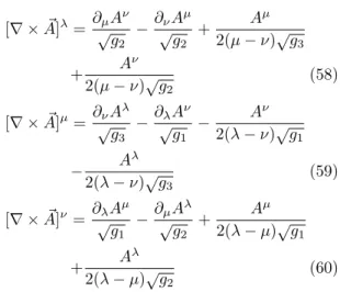
where thegi are defined in (50). The curl in components
is given by
[∇ ×A~]λ=∂µAν
√g
2 −
∂νAµ
√g
2
+ A
µ
2(µ−ν)√g3
+ A
ν
2(µ−ν)√g2
(58)
[∇ ×A~]µ=∂νAλ
√g
3 −
∂λAν
√g
1 −
Aν
2(λ−ν)√g1
− A
λ
2(λ−ν)√g3 (59)
[∇ ×A~]ν= ∂λAµ
√g
1 −
∂µAλ
√g
2
+ A
µ
2(λ−µ)√g1
+ A
λ
2(λ−µ)√g2 (60)
3.3. Other coordinate systems
The Cartesian coordinate system is the trivial one in which the orthonormal basis is identical to the coordinate basis and all commutators are zero.
The spherical coordinate system is one of the more important cases. To illustrate the use of programming codes in obtaining these operators in a very simple pro-cedural way, in [1] we make available a code to obtain the divergence and curl for the free software Maxima and also for Maple. Moreover, we also include a code to draw general coordinate systems both for Maxima and Maple [1].
All other coordinate systems are plotted and given in the following Table 1. In this Table some of the coordinate systems are described by Jacobi’s elliptic functions. These same coordinate systems could be described by square roots instead, the disadvantage is that it will be necessary a greater amount of charts to cover the EuclideanE3
space.
Table 1:These are the eight coordinate systems other than rectangular, cylindrical and spherical coordinates in which the Laplace operator is separable. It is not difficult to adapt the code given in [1] to each one of these coordinate systems or to any other situation of interest, and we leave this exercise to the reader.
Parabolic Elliptic Parabolic Paraboloidal
cylindrical cylindrical
x= 1
2 λ2−µ2
x=acoshµcosν x=λµcos(φ) x=dsn(
λ,κ)sn ν,κ′
cn(λ,κ)cn(µ,κ)
y=λµ y=asinhµsinν y=λµsin(φ) y=dsn(
µ,κ)cn ν,κ′
cn(λ,κ)cn(µ,κ)
z=z z=z z=1
2 λ2−µ2
z=d
2
hsn2(λ,κ)
cn2(λ,κ)−sn
2(µ,κ)
cn2(µ,κ)+dn 2
(ν,κ′)
k′2
i
λ∈Randµ∈R µ >0andν∈[0,2π) λ≥0,µ≥0,φ∈[0,2π) b=κa,√a2−b2=κ′a=√d λ >0,µ∈[−µ0, µ0],ν∈[−ν0, ν0]
Conical Ellipsoidal Prolate Oblate
x=rdn(λ, α)sn(µ, β) x=dsn(λ,κ)sn µ,κ ′dn(ν,κ)
cn(λ,κ) x=dsinh(µ) sin(θ) cos(φ) x=dcosh(µ) sin(θ) cos(φ)
y=rsn(λ, α)dn(µ, β) y=dcn
µ,κ′cn(ν,κ)
cn(λ,κ) y=dsinh(µ) sin(θ) sin(φ) y=dcosh(µ) sin(θ) sin(φ)
z=rcn(λ, α)cn(µ, β) z=adn(λ,κ)dn µ,κ ′sn
(ν,κ)
cn(λ,κ) z=dcosh(µ) cos(θ) z=dsinh(µ) cos(θ)
α2+β2= 1
b=κa,
p
a2−b2 =κ′a=d µ >0,θ∈[0, π],φ∈[0,2π) µ >0,θ∈[0, π],φ∈[0,2π] r >0,µ∈[−µ0, µ0], λ >0,µ∈[−µ0, µ0],
4. Final remarks
In the present work we approach the vectorial calculus through the use of the concept of non coordinate basis, especially the tetrad basis. We present here a practical development to obtain the divergence and curl, that have direct applications in physical problems, for example, in Electromagnetism, Fluid Mechanics, Gravitational Theories and other areas of Physics. The approach is restricted to Euclidean geometry, however, it can be easily extended to curved spaces, which also include situations with gravitational field.
In this sense, the purpose of this work complements the literature and at the same time introduces sophisticated mathematical concepts with direct applications. It is worth noting that the connection given by (26) and (33), could also be obtained through the Fock Ivanenko operator as a particular case when the spin is 1 [26].
Therefore, it is presented to the students, either late undergraduate or beginners graduate, a formalism more adapted to differential geometry and theoretical physics.
We thus consider the application of this method for the eleven coordinate systems mentioned in [4], for which the separation of variables can be applied to Laplace’s operator. For each of the eleven coordinates there is a cor-responding metric tensor, and tetrad basis and through the commutator of this basis the connection is obtained. With the appropriate connection, the divergence and curl for each of these eleven cases can be obtained. We work out in detail the case for the well known polar coordi-nates in section 3.1. In [1] we show an example code both for the algebraic manipulator Maple [24] an the free software Maxima [22], [23] to obtain the divergence and curl also for the well known spherical coordinates. Calcu-lations can be made by the reader, either manually, or by adapting the example code to the situation of interest.
Acknowledgements
We thank V. Toth in helping us with the Maxima code, and R. A. Müller for offering his website to host our codes. We must also thank the Referee for his patience and friendly suggestions.
References
[1] http://www.tele.ed.nom.br/ag/divergence.html [2] K.R. Symon, Mechanics (Addison-Wesley,
Mas-sachusetts, 1960), 2ª ed.
[3] D.J. Griffiths,Introduction to Electrodynamics (Prentice-Hall, New Jersey, 1999), 3ª ed.
[4] P.M. Morse and H. Feshbach,Methods of Theoretical Physics, Part I (Mc Graw-Hill, New York, 1953), p. 655. [5] J.W. Gibbs and E.B. WilsonVector Analysis(Charles
Scribner’s Sons, New York, 1901).
[6] A. Sommerfeld,Mechanics of Deformable Bodies - Lec-tures on Theoretical Physics Vol. II (Academic Press, Massachusetts, 1950).
[7] S. Hassani,Mathematical Methods for Students of Physics and Related Fields(Springer, New York, 2009), 2ª ed. [8] K.F. Riley, M.P. Hobson and S.J. Bence,
Mathemati-cal Methods for Physics and Engineering(Cambridge University Press, Cambridge, 2006), 3ª ed.
[9] G.B. Arfken and H.J. Weber,Mathematical Methods for Physicists(Elsevier, Buffalo Grove, 2005), 6ª ed. [10] E. Butkov,Mathematical Physics, (Addison-Wesle,
Mas-sachusetts, 1968).
[11] G. Arfken, H.J. Weber and F.E. HarrisMathematical Methods for Physicists(Elsevier, Buffalo Grove, 2013), 7ª ed.
[12] M.L. Boas,Mathematical Methods in the Physical Sci-ences(John Wiley & Sons, New Jersey, 1983), 2ª ed. [13] P.M. Morse and H. Feshbach, Methods of Theoretical
Physics, Part I (Mc Graw-Hill, New York, 1953). [14] H. Stephani, D. Kramer, M. MacCallum, C. Hoenselaers
and E. Herlt,Exact Solutions of Einstein’s Field Equa-tions(Cambridge University Press, Cambridge, 2003), 2ª ed.
[15] D. Felice and C.J.S. Clarke,Relativity on curved mani-folds(Cambridge University Press, Cambridge, 1990). [16] T. Dray,Differential Forms and the Geometry of General
Relativity(CRC Press, Boca Raton, 2014).
[17] C.W. Misner, K.S. Thorne and J.A. Wheeler,Gravitation (W.H. Freeman and Company, New York, 1973). [18] J.G. Darboux,Leçons sur la théorie générale des surfaces
et les applications géométriques du calcul infinitésimal (Gauthier-Villars, Paris, 1887-96).
[19] E. Cartan,La théorie des groupes finis et continus et la géométrie différentielle traitées par la méthode du repère mobile(Gauthier-Villars, Paris, 1937).
[20] https://en.wikipedia.org/wiki/Darboux_f rame
[21] T. Dray and C.A. Manogue, Am. J. Phys. 70, 1129 (2002).
[22] http://maxima.sourceforge.net/download.html [23] http://maxima.sourceforge.net/documentation.html [24] https://www.maplesoft.com
[25] P. Moon and D.E. Spencer, Field Theory Handbook (Springer-Verlag, Berlin, 1988).
[26] V. Fock and D. Iwanenko, Compt. Rend. Acad. Sci. Paris