The Casimir Effect: Some Aspects
Carlos Farina
Universidade Federal do Rio de Janeiro, Ilha do Fund ˜ao, Caixa Postal 68528, Rio de Janeiro, RJ, 21941-972, Brazil
Received on 10 August, 2006
We start this paper with a historical survey of the Casimir effect, showing that its origin is related to ex-periments on colloidal chemistry. We present two methods of computing Casimir forces, namely: the global method introduced by Casimir, based on the idea of zero-point energy of the quantum electromagnetic field, and a local one, which requires the computation of the energy-momentum stress tensor of the corresponding field. As explicit examples, we calculate the (standard) Casimir forces between two parallel and perfectly conducting plates and discuss the more involved problem of a scalar field submitted to Robin boundary conditions at two parallel plates. A few comments are made about recent experiments that undoubtedly confirm the existence of this effect. Finally, we briefly discuss a few topics which are either elaborations of the Casimir effect or topics that are related in some way to this effect as, for example, the influence of a magnetic field on the Casimir effect of charged fields, magnetic properties of a confined vacuum and radiation reaction forces on non-relativistic moving boundaries.
Keywords: Quantum field theory; Casimir effect
I. INTRODUCTION
A. Some history
The standard Casimir effect was proposed theoretically by the dutch physicist and humanist Hendrik Brugt Gerhard Casimir (1909-2000) in 1948 and consists, basically, in the attraction of two parallel and perfectly conducting plates lo-cated in vacuum [1]. As we shall see, this effect has its origin in colloidal chemistry and is directly related to the dispersive van der Waals interaction in the retarded regime.
The correct explanation for the non-retarded dispersive van der Walls interaction between two neutral but polariz-able atoms was possible only after quantum mechanics was properly established. Using a perturbative approach, London showed in 1930 [2] for the first time that the above mentioned interaction is given byVLon(r)≈ −(3/4)(ω0α2)/r6, where αis the static polarizability of the atom,ω0is the dominant transition frequency andris the distance between the atoms. In the 40’s, various experiments with the purpose of studying equilibrium in colloidal suspensions were made by Verwey and Overbeek [3]. Basically, two types of force used to be invoked to explain this equilibrium, namely: a repulsive elec-trostatic force between layers of charged particles adsorbed by the colloidal particles and the attractive London-van der Waals forces.
However, the experiments performed by these authors showed that London’s interaction was not correct for large dis-tances. Agreement between experimental data and theory was possible only if they assumed that the van der Waals interac-tion fell with the distance between two atoms more rapidly than 1/r6. They even conjectured that the reason for such a different behaviour for large distances was due to the retar-dation effects of the electromagnetic interaction (the informa-tion of any change or fluctuainforma-tion occurred in one atom should spend a finite time to reach the other one). Retardation ef-fects must be taken into account whenever the time interval
spent by a light signal to travel from one atom to the other is of the order (or greater) than atomic characteristic times (r/c≥1/ωMan, whereωmnare atomic transition frequencies). Though this conjecture seemed to be very plausible, a rigorous demonstration was in order. Further, the precise expression of the van der Waals interaction for large distances (retarded regime) should be obtained.
In the summer or autumn 1947 (but I am not ab-solutely certain that it was not somewhat earlier or later) I mentioned my results to Niels Bohr, during a walk.“That is nice”, he said, “That is something new.” I told him that I was puzzled by the extremely simple form of the expressions for the interaction at very large distance and he mumbled something about zero-point energy. That was all, but it put me on a new track.
Following Bohr’s suggestion, Casimir re-derived the results obtained with Polder in a much simpler way, by computing the shift in the electromagnetic zero-point energy caused by the presence of the atoms and the walls. He presented his result in theColloque sur la th´eorie de la liaison chimique, that took place at Paris in April of 1948:
I found that calculating changes of zero-point en-ergy really leads to the same results as the calcu-lations of Polder and myself...
A short paper containing this beautiful result was published in a French journal only one year later [6]. Casimir, then, decided to test his method, based on the variation of zero-point energy of the electromagnetic field caused by the interacting bodies in other examples. He knew that the existence of zero-point energy of an atomic system (a hot stuff during the years that followed its introduction by Planck [7]) could be inferred by comparing energy levels of isotopes. But how to produce isotopes of the quantum vacuum? Again, in Casimir’s own words we have the answer [8]:
if there were two isotopes of empty space you could really easy confirm the existence of the zero-point energy. Unfortunately, or perhaps for-tunately, there is only one copy of empty space and if you cannot change the atomic distance then you might change the shape and that was the idea of the attracting plates.
A month after theColloqueheld at Paris, Casimir presented his seminal paper [1] on the attraction between two parallel conducting plates which gave rise to the famous effect that since then bears his name:
On 29 May, 1948, ‘I presented my paper on the attraction between two perfectly conducting plates at a meeting of the Royal Netherlands Academy of Arts and Sciences. It was published in the course of the year...
As we shall see explicitly in the next section, Casimir ob-tained an attractive force between the plates whose modulus per unit area is given by
F(a)
L2 ≈0,013 1 (a/µm)4
dyn
cm2, (1)
whereais the separation between the plates, L2 the area of each plate (presumably very large,i.e.,L≫a).
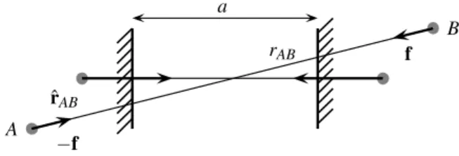
A direct consequence of dispersive van der Waals forces between two atoms or molecules is that two neutral but polar-izable macroscopic bodies may also interact with each other. However, due to the so called non-additivity of van der Waals forces, the total interaction potential between the two bodies is not simply given by a pairwise integration, except for the case where the bodies are made of a very rarefied medium. In principle, the Casimir method provides a way of obtaining this kind of interaction potential in the retarded regime (large distances) without the necessity of dealing explicitly with the non-additivity problem. Retarded van der Waals forces are usually called Casimir forces. A simple example may be in order. Consider two semi-infinite slabs made of polarizable material separated by a distancea, as shown in Figure 1.
a
A
B
ˆ rAB
−f
f
rAB
FIG. 1: Forces between molecules of the left slab and molecules of the right slab.
Suppose the force exerted by a moleculeAof the left slab on a moleculeBof the right slab is given by
fAB=−
C rγABrAB,
whereCandγare positive constants,rABthe distance between the molecules and ˆrABthe unit vector pointing fromAtoB. Hence, by a direct integration it is straightforward to show that, for the case of dilute media, the force per unit area be-tween the slabs is attractive and with modulus given by
Fslabs
Area = C′
aγ−4, (2)
whereC′is a positive constant. Observe that forγ=8, which corresponds to the Casimir and Polder force, we obtain a force between the slabs per unit area which is proportional to 1/a4. Had we used the Casimir method based on zero-point energy to compute this force we would have obtained precisely this kind of dependence. Of course, the numerical coefficients would be different, since here we made a pairwise integration, neglecting the non-additivity problem. A detailed discussion on the identification of the Casimir energy with the sum of van der Waals interaction for a dilute dielectric sphere can be found in Milton’s book [9] (see also references therein).
able to derive and predict several results, like the variation of the thickness of thin superfluid helium films in a remarkable agreement with the experiments [11]. The Casimir result for metallic plates can be reobtained from Lifshitz formula in the appropriate limit. The Casimir and Polder force can also be inferred from this formula [9] if we consider one of the media sufficiently dilute such that the force between the slabs may be obtained by direct integration of a single atom-wall inter-action [12].
The first experimental attempt to verify the existence of the Casimir effect for two parallel metallic plates was made by Sparnaay [13] only ten years after Casimir’s theoretical prediction. However, due to a very poor accuracy achieved in this experiment, only compatibility between experimental data and theory was established. One of the great difficulties was to maintain a perfect parallelism between the plates. Four decades have passed, approximately, until new experiments were made directly with metals. In 1997, using a torsion pendulum Lamoreaux [14] inaugurated the new era of experi-ments concerning the Casimir effect. Avoiding the parallelism problem, he measured the Casimir force between a plate and a spherical lens within the proximity force approximation [15]. This experiment may be considered a landmark in the history of the Casimir effect, since it provided the first reliable exper-imental confirmation of this effect. One year later, using an atomic force microscope , Mohideen and Roy [16] measured the Casimir force between a plate and a sphere with a better accuracy and established an agreement between experimen-tal data and theoretical predictions of less than a few percents (depending on the range of distances considered). The two precise experiments mentioned above have been followed by many others and an incomplete list of the modern series of ex-periments about the Casimir effect can be found in [17]-[26]. For a detailed analysis comparing theory and experiments see [27, 28]
We finish this subsection emphasizing that Casimir’s orig-inal predictions were made for an extremely idealized situ-ation, namely: two perfectly conducting (flat) plates at zero temperature. Since the experimental accuracy achieved nowa-days is very high, any attempt to compare theory and exper-imental data must take into account more realistic boundary conditions. The most relevant ones are those that consider the finite conductivity of real metals and roughness of the surfaces involved. These conditions become more important as the dis-tance between the two bodies becomes smaller. Thermal ef-fects must also be considered. However, in principle, these effects become dominant compared with the vacuum contri-bution for large distances, where the forces are already very small. A great number of papers have been written on these topics since the analysis of most recent experiments require the consideration of real boundary conditions. For finite con-ductivity effects see Ref. [30]; the simultaneous consideration of roughness and finite conductivity in the proximity for ap-proximation can be found in Ref. [31] and beyond PFA in Ref. [32] (see also references cited in the above ones). Concerning the present status of controversies about the thermal Casimir force see Ref. [29]
B. The Casimir’s approach
The novelty of Casimir’s original paper was not the predic-tion of an attractive force between neutral objects, once Lon-don had already explained the existence of a force between neutral but polarizable atoms, but the method employed by Casimir, which was based on the zero-point energy ot the elec-tromagnetic field. Proceeding with the canonical quantization of the electromagnetic field without sources in the Coulomb gauge we write the hamiltonian operator for the free radiation field as
ˆ H=
2
∑
α=1
∑
kωk
ˆ a†kαaˆkα+
1 2
, (3)
where ˆa†kαand ˆakαare the creation and annihilation operators
of a photon with momentumkand polarization α. The en-ergy of the field when it is in the vacuum state, or simply the vacuum energy, is then given by
E
0:=0|H|ˆ 0=∑
k
2
∑
α=1 1
2ωk, (4)
which is also referred to as zero-point energy of the electro-magnetic field in free space. Hence, we see that even if we do not have any real photon in a given mode, this mode will still contribute to the energy of the field with12ωkαand total vac-uum energy is then a divergent quantity given by an infinite sum over all possible modes.
The presence of two parallel and perfectly conducting plates imposes on the electromagnetic field the following boundary conditions:
E×nˆ|plates = 0
(5) B·nˆ|plates = 0,
which modify the possible frequencies of the field modes. The Casimir energy is, then, defined as the difference between the vacuum energy with and without the material plates. How-ever, since in both situations the vacuum energy is a divergent quantity, we need to adopt a regularization prescription to give a physical meaning to such a difference. Therefore, a precise definition for the Casimir energy is given by
E
Cas:=lim s→0
∑
kα
1 2ωk
I
−
∑
kα
1 2ωk
II
, (6)
its radius while the self-energy of a pair of plates is indepen-dent of the distance between them).
Observe that, in the previous definition, we eliminate the regularization prescription only after the subtraction is made. Of course, there are many different regularization methods. A quite simple but very efficient one is achieved by introducing a high frequency cut off in the zero-point energy expression, as we shall see explicitly in the next section. This procedure can be physically justified if we note that the metallic plates become transparent in the high frequency limit so that the high frequency contributions are canceled out from equation (6).
Though the calculation of the Casimir pressure for the case of two parallel plates is very simple, its determination may become very involved for other geometries, as is the case, for instance, of a perfectly conducting spherical shell. Af-ter a couple of years of hard work and a “nightmare in Bessel functions”, Boyer [33] computed for the first time the Casimir pressure inside a spherical shell. Surprisingly, he found a re-pulsive pressure, contrary to what Casimir had conjectured five years before when he proposed a very peculiar model for the stability of the electron [34]. Since then, Boyer’s result has been confirmed and improved numerically by many au-thors, as for instance, by Davies in 1972 [35], by Balian and Duplantier in 1978 [36] and also Milton in 1978 [37], just to mention some old results.
The Casimir effect is not a peculiarity of the electromag-netic field. It can be shown that any relativistic field under boundary conditions caused by material bodies or by a com-pactification of space dimensions has its zero-point energy modified. Nowadays, we denominate by Casimir effect any change in the vacuum energy of a quantum field due to any ex-ternal agent, from classical backgrounds and non-trivial topol-ogy to external fields or neighboring bodies. Detailed reviews of the Casimir effect can be found in [9, 38–41].
C. A local approach
In this section we present an alternative way of comput-ing the Casimir energy density or directly the Casimir pres-sure which makes use of a local quantity, namely, the energy-momentum tensor. Recall that in classical electromagnetism the total force on a distribution of charges and currents can be computed integrating the Maxwell stress tensor through an appropriate closed surface containing the distribution. For simplicity, let us illustrate the method in a scalar field. The lagrangian density for a free scalar field is given by
L
φ,∂µφ=−1 2∂µφ∂
µφ−1 2m
2φ2 (7)
The field equation and the corresponding Green function are given, respectively, by
(−∂2+m2)φ(x) = 0 ; (8)
(∂2−m2)G(x,x′) = −δ(x−x′), (9)
where, as usual,G(x,x′) =i0|T φ(x)φ(x′)|0.
Since the above lagrangian density does not depend explic-itly onx, Noether’s Theorem leads naturally to the following energy-momentum tensor (∂µTµν=0)
Tµν= ∂
L
∂(∂µφ)∂νφ+gµν
L
, (10)which, after symmetrization, can be written in the form
Tµν=
1
2 ∂µφ∂νφ+∂νφ∂µφ
+gµν
L
. (11)For our purposes, it is convenient to write the vacuum expec-tation value (VEV) of the energy-momentum tensor in terms of the above Green function as
0|Tµν(x)|0=−
i 2xlim′→x
(∂′µ∂ν+∂′ν∂µ)−gµν(∂′α∂α+m2)
G(x,x′).
(12) In this context, the Casimir energy density is defined as
ρC(x) =0|T00(x)|0BC− 0|T00(x)|0Free, (13) where the subscriptBCmeans that the VEV must be computed assuming that the field satisfies the appropriate boundary con-dition. Analogously, considering for instance the case of two parallel plates perpendicular to the
OZ
axis (the generaliza-tion for other configurageneraliza-tions is straightforward) the Casimir force per unit area on one plate is given byF
C=0|Tzz+|0 − 0|Tzz−|0, (14) where superscripts+and−mean that we must evaluateTzz on both sides of the plate. In other words, the desired Casimir pressure on the plate is given by the discontinuity ofTzzat the plate. Using equation (12),Tzzcan be computed by0|Tzz|0=−
i 2xlim′→x
∂
∂z
∂ ∂z′−
∂2
∂z2
G(x,x′). (15) Local methods are richer than global ones, since they pro-vide much more information about the system. Depending on the problem we are interested in, they are indeed neces-sary, as for instance in the study of radiative properties of an atom inside a cavity. However, with the purpose of comput-ing Casimir energies in simple situations, one may choose, for convenience, global methods. Previously, we presented only the global method introduced by Casimir, based on the zero-point energy of the quantized field, but there are many others, namely, the generalized zeta function method [42] and Schwinger’s method [43, 44], to mention just a few.
II. EXPLICIT COMPUTATION OF THE CASIMIR FORCE
introduced by Casimir which is based on the zero-point en-ergy. Then, we give a second example where we use a local approach, based on the energy-momentum tensor. We finish this section by sketching some results concerning the Casimir effect for massive fields.
A. The electromagnetic Casimir effect between two parallel plates
As our first example, let us consider the standard (QED) Casimir effect where the quantized electromagnetic field is constrained by two perfectly parallel conducting plates sepa-rated by a distancea. For convenience, let us suppose that one plate is located atz=0, while the other is located atz=a. The quantum electromagnetic potential between the metallic plates in the Coulomb gauge (∇·A=0) which satisfies the appropriate BC is given by [45]
A(ρ,z,t) = L
2
(2π)2
∞′
∑
n=0d2κ
2π
ckaL2 1/2
×
×
a(1)(κ,n)(κˆ×ˆz)sin nπz a
+
+ a(2)(κ,n)inπ kaκsin
nπz a
−ˆzκ
kcos nπz
a
× × ei(κ·ρ−ωt) +h.c. , (16) where ω(κ,n) =ck=c
κ2+n2π2/a21/2
, with n being a non-negative integer and the prime inΣ′means that forn=0 an extra 1/2 factor must be included in the normalization of the field modes. The non-regularized Casimir energy then reads
E
cnr(a) = c 2L2 d
2κ
(2π)2
κ+2
∞
∑
n=1
κ2+n2π2 a2
1/2
− c 2
L2 d
2κ
(2π)2 +∞
−∞
adkz 2π 2
κ2+k2
z.
Making the variable transformationκ2+ (nπ/a)2=:λand in-troducing exponential cutoffs we get a regularized expression (in 1948 Casimir used a generic cutoff function),
E
r(a,ε) =L2 2π 1 2 ∞ 0
e−εκκ2dκ+
∞
∑
n=1∞
nπ a
e−ελλ2dλ−
− ∞ 0 dn ∞ nπ a
e−ελλ2dλ =L 2 2π 1 ε3+
∞
∑
n=1∂2
∂ε2
e−εnπ/a
ε − − ∞ 0 dn∂ 2 ∂ε2 ∞ nπ a
e−ελdλ . (17) Using that ∂2 ∂ε2 1 ε ∞
∑
n=1e−εnπ/a = ∂ 2 ∂ε2 1 ε 1 eεπ/a−1
,
as well as the definition of Bernoulli’s numbers,
1 et−1 =
∞
∑
n=0Bn
tn−1 n! , we obtain
E
(a) = L2
2π
1 ε3+
∂2 ∂ε2 1 ε ∞
∑
n=0Bn n! επ a n−1 − 6a
πε4 = L 2 2π
6(B0−1)a π
1
ε4+ (1+2B1) 1 ε3+
B4 12 π a 3 + ∞
∑
n=5Bn
n! π
a n−1
(n−2)(n−3)εn−4
.
Using the well known valuesB0=1,B1=−12andB4=−301, and takingε→0+, we obtain
E
(a)L2 =−c
π2 24×30·
1 a3
As a consequence, the force per unit area acting on the plate atz=ais given by
F(a)
L2 =− 1 L2
∂
E
c(a) ∂a =−π2c
240a4 ≈ −0,013 1 (a/µm)4
dyn cm2, where in the last step we substituted the numerical values of and c in order to give an idea of the strength of the Casimir pressure. Observe that the Casimir force between the (conducting) plates is always attractive. For plates with 1cm2 of area separated by 1µm the modulus of this attrac-tive force is 0,013dyn. For this same separation, we have PCas≈10−8Patm, wherePatm is the atmospheric pressure at sea level. Hence, for the idealized situation of two perfectly conducting plates and assumingL2=1cm2, the modulus of the Casimir force would be≈10−7Nfor typical separations used in experiments. However, due to the finite conductivity of real metals, the Casimir forces measured in experiments are smaller than these values.
B. The Casimir effect for a scalar field with Robin BC
In order to illustrate the local method based on the energy-momentum tensor, we shall discuss the Casimir effect of a massless scalar field submitted to Robin BC at two parallel plates, which are defined as
φ|bound.=β ∂φ
where, by assumption,βis a non-negative parameter. How-ever, before computing the desired Casimir pressure, a few comments about Robin BC are in order.
First, we note that Robin BC interpolate continuously Dirichlet and Neumann ones. Forβ→0 we reobtain Dirichlet BC while forβ→∞we reobtain Neumann BC. Robin BC al-ready appear in classical electromagnetism, classical mechan-ics, wave, heat and Schr¨odinger equations [46] and even in the study of interpolating partition functions [47]. A nice realiza-tion of these condirealiza-tions in the context of classical mechanics can be obtained if we study a vibrating string with its extremes attached to elastic supports [48?]. Robin BC can also be used in a phenomenological model for a penetrable surfaces [49]. In fact, in the context of the plasma model, it can be shown that for frequencies much smaller than the plasma frequency (ω≪ωP)the parameterβplays the role of the plasma wave-length [? ]. In the context of QFT this kind of BC appeared more than two decades ago [50, 51]. Recently, they have been discussed in a variety of contexts, as in the AdS/CFT corre-spondence [52], in the discussion of upper bounds for the ratio entropy/energy in confined systems [53], in the static Casimir effect [54], in the heat kernel expansion [55–57] and in the one-loop renormalization of theλφ4theory [58, 59]. As we will see, Robin BC can give rise to restoring forces in the sta-tic Casimir effect [54].
Consider a massless scalar field submitted to Robin BC on two parallel plates:
φ|z=0=β1
∂φ
∂z|z=0 ; φ|z=a=−β2
∂φ
∂z|z=a, (19) where we assumeβ1(β2)≥0. For convenience, we write
G(x,x′) = d3k
α
(2π)3e
ıkα(x−x′)α
g(z,z′;k⊥,ω), (20) withα=0,1,2,gµν=diag(−1,+1,+1,+1)and the reduced
Green functiong(z,z′;k⊥,ω)satisfies ∂2
∂z2+λ 2
g(z,z′;k⊥,ω) =−δ(z−z′), (21) whereλ2=ω2−k2
⊥andg(z,z′;k⊥,ω)is submitted to the fol-lowing boundary conditions (for simplicity, we shall not write k⊥,ωin the argument ofg):
g(0,z′) =β1
∂ ∂zg(0,z
′) ; g(a,z′) =−β 2
∂ ∂zg(a,z
′)
It is not difficult to see thatg(z,z′)can be written as
g(z,z′) =
A(z′) (sinλz+β1λcosλz), z<z′ B(z′) (sinλ(z−a)−β2λcosλ(z−a)),z>z′
(22) For points inside the plates, 0<z,z′<a, the final expression for the reduced Green function is given by
gRR(z,z′) =− 1
γ1e
ıλz<−e−ıλz< 1
γ2e
ıλ(z>−a)−eıλ(z>−a) 2ıλ(γ1
1e ıλa−1
γ2e
−ıλa) , (23)
whereγi=11+−iiβiλβiλ(i=1,2). Outside the plates, withz,z′>a, we have:
gRR(z,z′) =e ıλ(z<−a)
2ıλ
1 γ2
eıλ(z<−a)−e−ıλ(z<−a). (24) Definingtµνsuch that
Tµν(x)= d2k
⊥
(2π)
dω 2πt
µν(x), (25)
we have
t33(z)= 1 2izlim′→z
∂
∂z
∂ ∂z′+λ
2
g(z,z′). (26) The Casimir force per unit area on the plate atx=ais given by the discontinuity int33:
F
= d2k⊥
(2π)
dω 2π
t33|z=a−− t
33|
z=a+
.
After a straightforward calculation, it can be shown that
F
(β1,β2;a) =− 1 32π2a4∞ 0
dξ ξ3 1+β1ξ/2a
1−β1ξ/2a
1+β2ξ/2a
1−β2ξ/2a
eξ−1
.
(27) Depending on the values of parametersβ1andβ2, restoring Casimir forces may arise, as shown in Figure 2 by the dotted line and the thin solid line.
pa
4a
O
(β1=0,β2→∞)
(β1=β2=0 orβ1=β2→∞) (β1=0,β2=1)
FIG. 2: Casimir pressure, conveniently multiplied bya4, as a func-tion ofafor various values of parametersβ1andβ2.
The particular cases of Dirichlet-Dirichlet, Neumann-Neumann and Dirichlet-Neumann-Neumann BC can be reobtained if we take, respectively,β1=β2=0, β1=β2→∞andβ1= 0 ;β2→∞. For the first two cases, we obtain
F
DD(a) =F
NN(a) =− 1 32π2a4∞ 0
dξ ξ
3
Using the integral representation ∞ 0 dξ
ξs−1
eξ−1 =ζR(s)Γ(s), whereζRis the Riemann zeta function, we get half the elec-tromagnetic result, namely,
F
DD(a) =F
NN(a) =−π 2c 4801
a4. (29)
For the case of mixed BC, we get
F
DN(a) = + 1 32π2a4∞ 0
dξ ξ
3
eξ+1 , (30) Using in the previous equation the integral representation ∞
0 dξ
ξs−1
eξ+1= (1−2
1−s)Γ(s)ζR(s)we get a repulsive pres-sure (equal to half of Boyer’s result [60] obtained for the elec-tromagnetic field constrained by a perfectly conducting plate parallel to an infinitely permeable one),
F
DN(a) =7 8×π2c 480
1
a4. (31)
C. The Casimir effect for massive particles
In this subsection, we sketch briefly some results concern-ing massive fields, just to get some feelconcern-ing about what kind of influence the mass of a field may have in the Casimir ef-fect. Firstly, let us consider a massive scalar field submit-ted to Dirichlet BC in two parallel plates, as before. In this case, the allowed frequencies for the field modes are given
byωk=c
κ2+n2π2 a2 +m2
1/2
, which lead, after we use the Casimir method explained previously, to the following result for the Casimir energy per unit area (see, for instance, Ref. [38])
1
L2
E
c(a,m) =− m2 8π2a∞
∑
n=11
n2K2(2amn), (32) whereKνis a modified Bessel function,mis the mass of the
field andais the distance between the plates, as usual. The limit of small mass,am≪1, is easily obtained and yields
1
L2
E
c(a,m)≈ −π2 1440a3+
m2
96a. (33)
As expected, the zero mass limit coincides with our previous result (29) (after the force per unit area is computed). Observ-ing the sign of the first correction on the right hand side of last equation we conclude that for small masses the Casimir effect is weakened.
On the other hand, in the limit of large mass,am≫1, it can be shown that
1
L2
E
c(a,m)≈ − m2 16π2aπ
ma 1/2
e−2ma (34) Note that the Casimir effect disappears form→∞, since in this limit there are no quantum fluctuations for the field any-more. An exponential decay withmais related to the plane
geometry. Other geometries may give rise to power law de-cays when ma→∞. However, in some cases, the behav-iour of the Casimir force withmamay be quite unexpected. The Casimir force may increase withmabefore it decreases monotonically to zero asma→∞(this happens, for instance, when Robin BC are imposed on a massive scalar field at two parallel plates [61]).
In the case of massive fermionic fields, an analogous be-haviour is found. However, some care must be taken when computing the Casimir energy density for fermions, regarding what kind of BC can be chosen for this field. The point is that Dirac equation is a first order equation, so that if we want non-trivial solutions, we can not impose that the field satis-fies Dirichlet BC at two parallel plates, for instance. The most appropriate BC for fermions is borrowed from the so called MIT bag model for hadrons [62], which basically states that there is no flux of fermions through the boundary (the normal component of the fermionic current must vanish at the bound-ary). The Casimir energy per unit area for a massive fermionic field submitted to MIT BC at two parallel plates was first com-puted by Mamayev and Trunov [63] (the massless fermionic field was first computed by Johnson in 1975 [64])
1 L2
E
f
c(a,m) =
− 1
π2a3 ∞
ma
dξ ξ
ξ2−m2a2log
1+ξ−ma ξ+mae
−2ξ. (35)
The small and large mass limits are given, respectively, by
1 L2
E
f
c(a,m) ≈ − 7π2 2880a3+
m 24a2; 1
L2
E
f
c(a,m) ≈ −
3(ma)1/2 25π3/2a3e
−2ma. (36)
Since the first correction to the zero mass result has an oppo-site sign, also for a fermionic field small masses diminish the Casimir effect. In the large mass limit,ma→∞, we have a behaviour analogous to that of the scalar field, namely, an ex-ponential decay withma(again this happens due to the plane geometry). We finish this section with an important observa-tion: even a particle as light as the electron has a completely negligible Casimir effect.
III. MISCELLANY
presence of material plates. Finally, we consider the so called dynamical Casimir effect.
A. Casimir effect under an external magnetic field
The Casimir effect which is observed experimentally is that associated to the photon field, which is a massless field. As we mentioned previously, even the electron field already ex-hibits a completely unmeasurable effect. With the purpose (and hope) of enhancing the Casimir effect of electrons and positrons we considered the influence of an external elec-tromagnetic field on their Casimir effect. Since in this case we have charged fields, we wondered if the virtual electron-positron pairs which are continuously created and destroyed from the Dirac vacuum would respond in such a way that the corresponding Casimir energy would be greatly amplified. This problem was considered for the first time in 1998 [65] (see also Ref. [66]). The influence of an external magnetic field on the Casimir effect of a charged scalar field was con-sidered in Ref. [67] and recently, the influence of a magnetic field on the fermionic Casimir effect was considered with the more appropriate MIT BC [68].
For simplicity, let us consider a massive fermion field un-der anti-periodic BC (in the
OZ
direction) in the presence of a constant and uniform magnetic field in this same direc-tion. After a lengthy but straightforward calculation, it can be shown that the Casimir energy per unit area is given by [66]E
(a,B)ℓ2 = −
2(am)2
π2a3
∞
∑
n=1(−1)n−1
n2 K2(amn) − eB
4π2a
∞
∑
n=1(−1)n−1 ∞ 0
dσe−(n/2)2σ−(am)2/σL eBa2
σ
,
where we introduced the Langevin function: L(ξ) =cothξ− 1/ξ. In the strong field limit, we have
E
(a,B)ℓ2 ≈ −
eBm
π2
∞
∑
n=1(−1)n−1
n K1(amn). (37) In this limit we can still analyze two distinct situations, namely, the small mass limit (ma≪1) and the large mass limit (ma≫1). Considering distances between the plates typ-ical of Casimir experiments (a≈1µm), we have in the former case
ρc(a,B) ρc(a,0)≈10
−4× B
Tesla ; ma≪1, (38) while in the latter case,
ρc(a,B) ρc(a,0) ≈10
−10× B
Tesla ; ma≫1. (39) In the above equationsρc(a,B)andρc(a,0)are the Casimir energy density under the influence of the magnetic field and without it, respectively. Observe that for the Casimir ef-fect of electrons and positrons, which must be treated as the
large mass limit described previously, huge magnetic fields are needed in order to enhance the effect (far beyond accessi-ble fields in the laboratory). In other words, we have shown that though the Casimir effect of a charged fermionic field can indeed be altered by an external magnetic field, the universal constants conspired in such a way that this influence turns out to be negligible and without any chance of a direct measure-ment at the laboratory.
B. Magnetic permeability of the constrained Dirac vacuum
In contrast to the classical vacuum, the quantum vacuum is far from being an empty space, inert and insensible to any external influence. It behaves like a macroscopic medium, in the sense that it responds to external agents, as for example electromagnetic fields or the presence of material plates. As previously discussed, recall that the (standard) Casimir effect is nothing but the energy shift of the vacuum state of the field caused by the presence of parallel plates. There are many other fascinating phenomena associated to the quantum vac-uum, namely, the particle creation produced by the application of an electric field [69], the birefringence of the QED vacuum under an external magnetic field [70, 71] and the Scharnhorst effect [72, 73], to mention just a few. This last effect pre-dicts that the velocity of light propagating perpendicularly to two perfectly conducting parallel plates which impose (by as-sumption) BC only on the radiation field is slightly altered by the presence of the plates. The expected relative variation in the velocity of light for typical values of possible experiments is so tiny (∆c/c≈10−36) that this effect has not been con-firmed yet. Depending on the nature of the material plates the velocity of light propagating perpendicular to the plates is ex-pected to diminish [74]. The Scharnhorst effect inside a cavity was considered in [75].
The negligible change in the velocity of light predicted by Scharnhorst may be connected with the fact that the effect that bears his name is a two-loop QED effect, since the classical field of a traveling light wave interacts with the radiation field only through the fermionic loop.
With the purpose of estimating a change in the constitutive equations of the quantum vacuum at the one-loop level, we were led to consider the fermionic field submitted to some BC. The magnetic permeabilityµof the constrained Dirac vacuum was computed by the first time in Ref. [76], but with the non-realistic anti-periodic BC. In this case, the result found for the relative change in the permeability,∆µ:=µ−1, was also neg-ligible (an analogous calculation has also been made in the context of scalar QED [77]). However, when the more real-istic MIT BC are imposed on the Dirac field at two parallel plates things change drastically. In this case, it can be shown that the magnetic permeability of the constrained Dirac vac-uum is given by [78]
1
µ(ma)=1− π−2 12π2
e2 ma+
1 6π2
e2
where
H(ma) = ∞
1
dx x
(x2−1)3/2ln
1+
x−1 x+1
e−2max
.
(40) For confining distances of the order of 0,1µm, we have
∆µ:=µ−1≈10−9. (41) The previous value is comparable to the magnetic permeabil-ity of Hydrogen and Nitrogen at room temperature and at-mospheric pressure. Hence, an experimental verification of this result seems to be not unfeasible (we will come back to this point in the final remarks).
C. The Dynamical Casimir effect
As our last topic, we shall briefly discuss the so called dy-namical Casimir effect, which consists, as the name suggests, of the consideration of a quantum field in the presence of moving boundaries. Basically, the coupling between vacuum fluctuations and a moving boundary may give rise to dissi-pative forces acting on the boundary as well as to a particle creation phenomenon. In some sense, these phenomena were expected. Recall that the static Casimir force is a fluctuat-ing quantity [79] and hence, usfluctuat-ing general arguments related to the fluctuation-dissipation theorem [80] dissipative forces on moving boundaries are expected. Further, using arguments of energy conservation we are led to creation of real parti-cles (photons, if we are considering the electromagnetic field [81]). For the above reasons, this topic is sometimes referred to as radiation reaction force on moving boundaries.
After Schwinger’s suggestion that the phenomenon of sonoluminescence could be explained by the dynamical Casimir effect [82] (name coined by himself), a lot of work has been done on this subject. However, it was shown a few years later that this was not the case (see [9] and references therein for more details).
The dynamical Casimir effect already shows up in the case of one (moving) mirror [83–85]. However, oscillating cavi-ties whose walls perform vibrations in parametric resonance with a certain unperturbed field eigenfrequency may greatly enhance the effect [86–89]. Recently, a one dimensional os-cillating cavity with walls of different nature was considered [90]. The dynamical Casimir effect has also been analyzed for a variety of three-dimensional geometries, including parallel plane plates [91], cylindrical waveguides [92], and rectangular [93], cylindrical [94] and spherical cavities [95]. For a review concerning classical and quantum phenomena in cavities with moving boundaries see Dodonov [96] and for a variety of top-ics on non-stationary Casimir effect including perspectives of its experimental verification see the special issue [97].
In this section, we shall discuss the force exerted by the quantum fluctuations of a massless scalar field on one moving boundary as well as the particle creation phenomenon in a un-usual example in 1+1 dimensions, where the field satisfies a Robin BC at the moving boundary [98, 99]. We shall follow
throughout this paper the perturbative method introduced by Ford and Vilenkin [84]. This method was also applied suc-cessfully to the case of the electromagnetic field under the influence of one moving (perfectly) conducting plate [85] as well as an oscillating cavity formed by two parallel (perfectly) conducting plates [91].
Let us then consider a massless scalar fieldφin 1+1 in the presence of one moving boundary which imposes on the field a Robin BC at one moving boundary when observed from a co-moving inertial frame. By assumption, the movement of the boundary is prescribed, non-relativistic and of small amplitude (δq(t)is the position of the plate at a generic in-stantt). Last assumptions may be stated mathematically by |δq˙(t)|<<c and |δq(t)|<<c/ω0,whereω0corresponds to the (main) mechanical frequency. Therefore, we must solve the following equation:∂2φ(x,t) =0, with the field satisfying a Robin BC at the moving boundary given by
∂
∂x+δq˙(t)
∂ ∂t
φ(x,t)|x=δq(t)= 1
βφ(x,t)|x=δq(t). (42) whereβis a non-negative parameter and the previous condi-tion was already written in the laboratory frame. We are ne-glecting terms of the order
O
(δq˙2/c2). The particular cases of Dirichlet and Neumann BC are reobtained by makingβ=0 andβ→∞, respectively. The dissipative forces for these par-ticular cases were studied at zero temperature as well as at finite temperature and also with the field in a coherent state in [100] (dissipative forces on a perfectly conducting mov-ing plate caused by the vacuum fluctuations of the electro-magnetic field at zero and non-zero temperature were studied in [101]). The perturbative approach introduced by Ford and Vilenkin [84] consists in writingφ(x,t) =φ0(x,t) +δφ(x,t), (43) whereφ0(x,t)is the field submitted to a Robin BC at a sta-tic boundary fixed at the origin andδφ(x,t)is the first order contribution due to the movement of the boundary. The total force on the moving boundary may be computed with the aid of the corresponding energy-momentum tensor, namely,
δF(t) =0|T11
t,δq+(t) −T11
t,δq−(t)
|0, (44) where superscripts+and−mean that we must compute the energy-momentum tensor on both sides of the moving bound-ary. It is convenient to work with time Fourier transforms. The susceptibilityχ(ω)is defined in the Fourier space by
δ
F
(ω) =:χ(ω)δQ(ω) (45)whereδ
F
(ω)andδQ(ω)are the Fourier transformations of δF(t)andδq(t), respectively. It is illuminating to compute the total work done by the vacuum fluctuations on the moving boundary. It is straightforward to show that+∞
−∞ δF(t)δq˙(t)dt=−
1 π
∞ 0
hence it is closely related with the total energy converted into real particles. On the other hand, the real part ofχ(ω), when it exists, does not contribute to the total work and hence it is not related to particle creation, but to dispersive effects. For the particular cases of Dirichlet or Neumann BC it can be shown that the susceptibility is purely imaginary and given by
χD(ω) =χN(ω) =iω3
6πc2 , (47)
which implies
δF(t) = 6πc2
d3
dt3δq(t). (48) Since
I
mχ(ω)>0, for these cases the vacuum fluctuations are always dissipating energy from the moving boundary.However, for Robin BC an interesting thing happens. It can be shown thatχ(ω)acquires also a real part, which gives rise to a dispersive force acting on the moving boundary. The explicit expressions of
R
eχ(ω) andI
mχ(ω) can be found in [98], but the general behaviour of them as functions of ω is shown in Figure 3. For convenience, we normalize these quantities dividing them by the valueI
mχD(ω), where the subscript Dmeans thatI
mχ(ω)must be computed with Dirichlet BC.FIG. 3: Imaginary and real parts ofχ(ω)with Robin BC appropri-ately normalized by the value ofImχ(ω)for the Dirichlet BC.
Now, let us discuss briefly the particle creation phenom-enon under Robin BC. Here, we shall consider a semi-infinite slab extending from−∞toδq(t)following as before a pre-scribed non-relativistic motion which imposes on the field Robin BC atδq(t). It can be shown that the corresponding spectral distribution is given by [99]
dN dω(ω) =
4ω 1+β2ω2
∞ 0
dω′ 2π
[δQ(ω−ω′)]2 1+β2ω′2 ω
′
1−β2ωω′ 2
(49) As an explicit example, let us consider the particular motion
δq(t) =δq0e−|t|/T cos(ω0t), (50)
where, by assumption,ω0T≫1 (this is made in order to sin-gle out the effect of a given Fourier component of the motion). For this case, we obtain the following spectral distribution
dN
dω(ω)= (δq0)
2Tω(ω
0−ω)× × [1−β
2ω(ω 0−ω)]2
(1+β2ω2)(1+β2(ω 0−ω)2)
Θ(ω0−ω). (51)
The spectral distributions for the particular cases of Dirichlet or Neumann BC can be easily reobtained by making simply β=0 andβ→∞, respectively. The results coincide and are given by [102] (we are makingc=1)
dN(D) dω (ω) =
dN(N)
dω (ω) = (δq0)
2Tω(ω
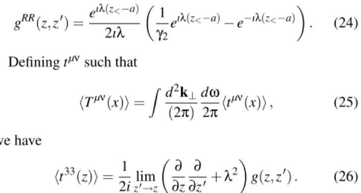
0−ω)Θ(ω0−ω). (52) A simple inspection in (51) shows that, due to the presence of the Heaviside step function, only the field modes with eigen-frequencies smaller than the mechanical frequency are ex-cited. Further, the number of particles created per unit fre-quency when Robin BC are used is always smaller than the number of particles created per unit frequency when Dirichlet (or Neumann) BC are employed.
FIG. 4: Spectral distributions of created particles for: Dirichlet and Neumann BC (dashed line) and for some interpolating values of the parameterβ(dotted and solid lines).
Figure 4 shows the spectral distribution for different val-ues of the parameterβ, includingβ=0 (dashed line), which corresponds to Dirichlet or Neumann BC. Note that for inter-polating values ofβ particle creation is always smaller than forβ=0 (dotted line). Depending on the value ofβ, particle creation can be largely suppressed (solid line).
IV. FINAL REMARKS
chemistry, an essentially experimental science. As we men-tioned previously, the novelty of Casimir’s seminal work [1] (see also [6]) was the technique employed by him to compute forces between neutral bodies as is emphasized by Itzykson and Zuber [103]:
By considering various types of bodies influenc-ing the vacuum configuration we may give an interesting interpretation of the forces acting on them.
However, the attractive or repulsive character of the Casimir force can not be anticipated. It depends on the specific bound-ary conditions, the number of space-time dimensions, the na-ture of the field (bosonic or fermionic), etc. The “mystery” of the Casimir effect has intrigued even proeminent physicists such as Julian Schwinger, as can be seen in his own statement [37]:
... one of the least intuitive consequences of quan-tum electrodynamics.
There is no doubt nowadays about the existence of the (sta-tic) Casimir effect, thanks to the vast list of accurate exper-iments that have been made during the last ten years. It is worth emphasizing that a rigorous comparison between the-ory and experimental data can be achieved only if the effects of temperature and more realistic BC are considered. In prin-ciple, the former are important in comparison with the vac-uum contribution for large distances, while the latter can not be neglected for short distances. Typical ranges investigated in Casimir experiments are form 0.1µmto 1.0µmand, to have an idea of a typical plasma wavelengths (the plasma wave-length is closely related to the penetration depth), recall that for Au we haveλP≈136nm.
The Casimir effect has become an extremely active area of research from both theoretical and experimental points of view and its importance lies far beyond the context of QED. This is due to its interdisciplinary character, which makes this effect find applications in quantum field theory (bag model, for instance), cavity QED, atomic and molecular physics, mathematical methods in QFT (development of new regular-ization and renormalregular-ization schemes), fixing new constraints in hypothetical forces, nanotechnology (nanomachines oper-ated by Casimir forces), condensed matter physics, gravitation and cosmology, models with compactified extra-dimensions, etc.
In this work, we considered quantum fields interacting only with classical boundaries. Besides, these interactions were described by highly idealized BC. Apart from this kind of in-teraction, there was no other interaction present. However,
the fields in nature are interacting fields, like those in QED, etc. Hence, we could ask what are the first corrections to the Casimir effect when we consider interacting fields. In princi-ple, they are extremely small. In fact, for the case of QED, the first radiative correction to the Casimir energy density (con-sidering that the conducting plates impose BC only on the ra-diation field) was firstly computed by Bordaget al[104] and is given by
E
C(1)(a,α) =E
C(0)(a)32
9
αλ
a
c, whereλcis the Comp-ton wavelength of the electron andE
C(0)(a)is the zeroth order contribution to the Casimir energy density. As we see, at least for QED, radiative corrections to the Casimir effect are exper-imentally irrelevant. However, they might be relevant in the bag model, where for quarksλc≈aand also the quark prop-agators must be considered submitted to the bag BC [9]. Be-sides, the study of radiative corrections to the Casimir effect provide a good laboratory for testing the validity of idealized BC in higher order of perturbation theory.Concerning the dynamical Casimir effect, the big challenge is to conceive an experiment which will be able to detect real photons created by moving boundaries or by an equivalent physical system that simulates rapid motion of a boundary. An ingenious proposal of an experiment has been made recently by the Padova’s group [105]. There are, of course, many other interesting aspects of the dynamical Casimir effect that has been studied, as quantum decoherence [106], mass correction of the moving mirrors [107], etc. (see also the reviews [108]).
As a final comment, we would like to mention that surpris-ing results have been obtained when a deformed quantum field theory is considered in connection with the Casimir effect. It seems that the simultaneous assumptions of deformation and boundary conditions lead to a new mechanism of creation of real particles even in a static situation [109]. Of course, the Casimir energy density is also modified by the deformation [110]. Quantum field theories with different space-time sym-metries, other than those governed by the usual Poincar´e al-gebra (as for example theκ-deformed Poincar´e algebra [111]) may give rise to a modified dispersion relation, a desirable fea-ture in some tentative models for solving recent astrophysical paradoxes.
Acknowledgments: I am indebted to B. Mintz, P.A. Maia Neto and R. Rodrigues for a careful reading of the manuscript and many helpful suggestions. I would like also to thank to all members of the Casimir group of UFRJ for enlightening dis-cussions that we have maintained over all these years. Finally, I thank to CNPq for a partial financial support.
[1] H.B.G. Casimir Proc. K. Ned. Akad. Wet.51, 793 (1948). [2] F. London Z. Physik63, 245 (1930).
[3] E.J.W. Vervey, J.T.G. Overbeek, and K. van Nes, J. Phys. and Colloid Chem.51, 631 (1947).
[4] H.B.G. Casimir and D. Polder, Phys. Rev.73, 360 (1948).
[5] D. Tabor and R.H.S. Winterton, Nature219, 1120 (1968); Proc. Roy. soc. Lond. A312, 435 (1969).
Casimir effect, in theProceedings of the Fourth Workshop on Quantum Field Theory under the Influence of External Condi-tions, pg 3, Ed. M. Bordag, World Scientific (1999).
[9] K.A. Milton,Physical Manifestation of zero point energy - The Casimir effect, World Scientific (2001).
[10] Lifshitz E M 1956Sov. Phys.JETP 273
E.M. Lifshtz e L.P. Pitaevskii,Landau and Lifshtz Course of Theoretical Physics: Statistical Physics Part 2, Butterworth-Heinemann (1980).
[11] E.S. Sabisky and C.H. Anderson, Phys. Rev. A7, 790 (1973). [12] Dzyaloshinskii I E Lifshitz, and L.P. Pitaevskii, Advan. Phys.
10, 165 (1961).
[13] M.J. Sparnaay, Physica24, 751 (1958). [14] S.K. Lamoreaux, Phys. Rev. Lett.78, 5 (1997).
S.K. Lamoreaux, Phys. Rev. Lett.81, 5475(E) (1998). [15] J. Blocki, J. Randrup, W.J. Swiatecki, and C.F. Tsang, Ann.
of Phys.105427 (1977).
[16] U. Mohideen e A. Roy, Phys. Rev. Lett.81, 4549 (1998). [17] G.L. Klimchiskaya, A. Roy, U. Mohideen, and V.M.
Mostepa-nenko Phys. Rev. A60, 3487 (1999).
[18] A. Roy and U. Mohideen, Phys. Rev. Lett.82, 4380 (1999) . [19] A. Roy, C.-Y. Lin e U. Mohideen, Phys. Rev. D60, 111101(R)
1999
[20] U. Mohideen e A. Roy, Phys. Rev. Lett.83, 3341 (1999). . [21] B.W. Harris, F. Chen e U. Mohideen, Phys. Rev. A62, 052109
(2000).
[22] F. Chen, U. Mohideen, G.L. Klimchitskaya, and V.M. Mostepanenko, Phys. Rev. A69, 022117 (2002).
[23] T. Ederth, Phys. Rev. A62, 062104 (2000) .
[24] G. Bressi, G. Carugno, R. Onofrio e G. Ruoso, Phys. Rev. Lett.88, 041804 (2002).
[25] F. Chen, U. Mohideen, G.L. Klimchitskaya, and V.M. Mostepanenko, Phys. Rev. Lett.88, 101801 (2002).
F. Chen, U. Mohideen, G.L. Klimchitskaya, and V.M. Mostepanenko, Phys. Rev. A66,032113 (2002).
[26] R.S. Decca, E. Fischbach, G.L. Klimchitskaya, D.E. Krause, D. Lopes e V. M. Mostepanenko Phys. Rev. D68, 116003 (2003).
[27] R.S. Decca, D. Lopez, E. Fischbach, G.L. Klimchitskaya, D.E. Krause, and V.M. Mostepanenko, Annals Phys. (NY)318, 37 (2005).
[28] G.L.Klimchitskaya, F.Chen, R.S.Decca, E.Fischbach, D.E. Krause, D.Lopez, U.Mohideen, and V.M.Mostepanenko, J. Phys. A39, 6485 (2006).
[29] V.M.Mostepanenko, V.B.Bezerra, R.S.Decca, B.Geyer, E.Fischbach, G.L.Klimchitskaya, D.E.Krause, D.Lopez, and C.Romero, J.Phys. A39, 6589 (2006).
[30] A. Lambrecht and S. Reynaud, Eur. Phys. J. D8, 309 (2000). [31] G.L. Klimchitskaya, A. Roy, U. Mohideen, and V.M.
Mostepanenko, Phys. Rev. A60, 3487 (1999).
[32] P.A. Maia Neto, A. Lambrecht, and S. Reynaud, Phys. Rev. A 72, 012115 (2005).
[33] T.H. Boyer, Phys. Rev.174, 1764 (1968). [34] H.B.G. Casimir, Physica19, 846 (1953). [35] B. Davies, J. Math. Phys.13, 1324 (1972)
[36] R. Balian and B. Duplantier, Ann. Phys. (N.Y.) 112, 165 (1978).
[37] K.A. Milton, L.L. DeRaad, , Jr., and J. Schwinger, Ann. Phys. (N.Y.)115, 1 (1978).
[38] G. Plunien, B. Muller, and W. Greiner Phys. Rep.134, 89 (1986).
[39] P.W. Milonni, The Quantum Vacuum: An Introduction to Quantum Electrodynamics, Academic, New York, (1994). [40] V.M. Mostepanenko and N.N. Trunov,The Casimir Effect and
its Applications, Clarendon Press, Oxford (1997).
[41] M. Bordag, U. Mohideen, e V. M. Mostepanenko, Phys. Rep. 353, 1 (2001).
[42] E. Elizalde, S. D. Odintsov, A. Romeo, A. A. Bitsenko, and S. Zerbini,Zeta Regularization Techniques with Applications, (World Scientific, Singapore, 1994).
[43] J. Schwinger, Lett. Math. Phys.24, 59 (1992).
[44] M.V. Cougo-Pinto, C. Farina, A. J. Segu´ı-Santonja, Lett. Math. Phys.30, 169 (1994);
M.V. Cougo-Pinto, C. Farina, A. J. Segu´ı-Santonja, Lett. Math. Phys.31, 309 (1994);
L.C. Albuquerque, C. Farina, S.J. Rabello e A.N. Vaidya, Lett. Math. Phys.34, 373 (1995).
[45] G. Barton, Proc. R. Soc. Lond. (1970).
[46] J.D. Bondurant and S.A. Fulling, J. Phys. A: Math. Gen.38, 1505 (2005).
[47] M. Asorey, F.S. da Rosa, and L.B. Carvalho, presented in the XXV ENFPC, Caxamb´u, Brasil (2004).
[48] G. Chen and J. Zhou,Vibration and Damping in Distributed Systems, ol.1(Boca Raton, FL:CRC), pg 15.
[49] V.M. Mostepanenko and N.N. Trunov, Sov. J. Nucl. Phys.45, 818 (1985).
[50] D. Deutsch and P. Candelas, Phys. Rev. D20, 3063 (1979). [51] G. Kennedy, R. Critchley, and J.S. Dowker, Ann. Phys. (NY)
125, 346 (1980).
[52] P. Minces and V.O. Rivelles, Nucl. Phys. B572, 651 (200) [53] S.N. Solodukhin, Phys. Rev. D63, 044002 (2001). [54] A. Romeo and A.A. Saharian, J. Phys. A35, 1297 (2002). [55] M. Bordag, H. Falomir, E.M. Santangelo, and D.V.
Vassile-vich, Phys. Rev. D65, 064032 (2002). [56] S.A. Fulling, J. Phys. A36, 6857 (2003). [57] J.S. Dowkermath.SP/0409442 v4(2005).
[58] L.C. de Albuquerque and R.M. Cavalcanti J. Phys. A37, 7039 (2004).
[59] L.C. de Albuquerque,hep-th/0507019 v1(2005). [60] T.H. Boyer, Phys. Rev A9, 2078 (1974).
[61] T.M. Britto, C. Farina, and F.P. Reis, in preparation.
[62] A. Chodos, R.L. Jaffe, K. Johnson, C.B. Thorn, and V.F. Weis-skopf, Phys. Rev. D9, 3471 (1974).
[63] S.G. Mamayev and N.N. Trunov, Sov. Phys. J.23, 551 (1980). [64] K. Johnson, Acta Pol. B6, 865 (1975).
[65] M.V. Cougo-Pinto, C. Farina, and A.C. Tort,Proceedings of the IV Workshop on Quantum Field Theory under the Influ-ence of External Conditions, Ed. M. Bordag, Leipzig, Ger-many, 1998.
[66] M.V. Cougo-Pinto, C. Farina, and A.C. Tort, Braz. J. Phys. 31, 84 (2001).
[67] M.V. Cougo-Pinto, C. Farina, M.R. Negr˜ao, and A. Tort, J. Phys. A32, 4457 (1999).
[68] E. Elizalde, F.C. Santos, and A.C. Tort, J. Phys. A35, 7403 (2002).
[69] J. Schwinger, Phys. Rev.82, 664 (1951).
[70] Z. Bialynicki-Birula and I. Bialynicki-Birula, Phys. Rev. D2, 2341 (1970).
[71] S.L. Adler, Ann. Phys. (NY)67, 599 (1971). [72] K. Scharnhorst, Phys. Lett. B236, 354 (1990). [73] G. Barton, PHys. Lett. B237, 559 (1990).
[74] M.V. Cougo-Pinto, C. Farina, F.C. Santos, and A.C. Tort, Phys. Lett. B (1998).
[75] R.B. Rodrigues and N.F. Svaiter, Physica A342, 529 (2004). [76] M.V. Cougo-Pinto, C. Farina, A.C. Tort, and J. Rafelski, Phys.
Lett. B434, 388 (1998).
[78] L. Bernardino, R. Cavalcanti, M.V. Cougo-Pinto, and C. Fa-rina, to appear in the J. Phys. A.
[79] G. Barton, J. Phys. A24, 5533 (1991); C. Eberlein, J. Phys. A25, 3015 (1992).
[80] V.B. Braginsky and F.Ya. Khalili, Phys. Lett. A161, 197 (1991);
M.T. Jaekel and S. Reynaud, Quant. Opt.4,39 (1992). [81] G.T. Moore, Math. Phys.112679 (1970).
[82] J. Schwinger, Proc. R. Soc. Lond.90, 958 (1993).
[83] S.A. Fulling and P.C.W. Davies, Proc. R. Soc. London A348, 393 (1976).
[84] L.H. Ford and A. Vilenkin, Phys. Rev. D25, 2569 (1982). [85] P.A. Maia Neto, J. Phys. A27, 2167 (1994);
P. A. Maia Neto and L.A.S. Machado, Phys. Rev. A54, 3420 (1996).
[86] C.K. Law, Phys. Rev. A49, 433 (1994). [87] V.V. Dodonov, Phys. Lett. A207, 126 (1995).
[88] A. Lambrecht, M.-T. Jaekel, and S. Reynaud, Phys. Rev. Lett. 77, 615 (1996).
[89] V.V. Dodonov and A.B. Klimov, Phys. Rev. A53, 2664 (1996).
[90] D.T. Alves, E.R. Granhen, and C. Farina, Phys. Rev. A,73, 063818 (2006).
[91] D.F. Mundarain and P.A. Maia Neto, Phys. Rev. A57, 1379 (1998).
[92] P.A. Maia Neto, J. Opt. B: Quantum and Semiclass. Opt.7, S86 (2005).
[93] V.V. Dodonov and A.B. Klimov, Phys. Rev. A 53, 2664 (1996).
M. Crocce, D.A.R. Dalvit and F.D. Mazzitelli, Phys. Rev. A 64, 013808 (2001).
G. Schaller, R. Sch¨utzhold, G. Plunien, and G. Soff, Phys. Rev. A66, 023812 (2002).
[94] M. Crocce, D.A.R. Dalvit, F.C. Lombardo, and F.D. Mazz-itelli, J. Opt. B: Quantum and Semiclass. Opt.7, S32 (2005). [95] C. Eberlein, Phys. Rev. Lett.76, 3842 (1996);
F.D. Mazzitelli and X.O. Milln, Phys. Rev. A 73, 063829 (2006).
[96] V.V. Dodonov, in: M.W. Evans (Ed.),Modern Nonlinear Op-tics, Advances in Chem. Phys. Series119, 309 (Wiley, New York, 2001).
[97] Special Issue on the Nostationary Casimir effect and quantum systems with moving boundaries J. Opt. B: Quantum Semi-class. Opt.7S3, (2005).
[98] B. Mintz, C. Farina, P.A. Maia Neto and R. Rodrigues, J.
Phys. A39, 6559 (2006).
[99] B. Mintz, C. Farina, P.A. Maia Neto and R. Rodrigues, J. Phys. A39, 11325 (2006).
[100] D.T. Alves, C. Farina and P.A. Maia Neto, J. Phys. A36, 11333 (2003).
[101] L.A. Machado, P.A. Maia Neto and C. Farina, Phys. Rev. D 66, 105016 (2002);
P.A. Maia Neto and C. Farina, Phys. Rev. Lett.,93, 59001 (2004).
[102] A. Lambbrecht, M.T. Jaekel and S. Reynaud, Phys. Rev. Lett. 77, 615 (1996).
[103] Claude Itzykson and Jean-Bernard Zuber, Quantum Field Theory, McGraw-Hill Book Company, New York (1980). [104] M. Bordag, D. Robaschik, and E. Wieczorek, Ann. Phys.
(NY)165, 192 (1985).
[105] C. Braggio, G. Bressi, G. Carugno, C. Del Noce, G. Galeazzi, A. Lombardi, A. Palmieri, G. Ruoso, D. Zanello, Europhys. Lett.70(6), 754 (2005).
[106] D. Dalvit and P.A. Maia Neto, Phys. Rev. Lett.84, 798 (2000); P.A. Maia Neto and D. Dalvit, Phys. Rev. A 62, 042103 (2000).
[107] M.T. Jaekel and S. Reynaud, Phys. Lett. A180, 9 (1993); G. Barton and A. Calogeracos, Ann. Phys. (NY)238, 227 (1995);
A. Calogeracos and G. Barton, Ann. Phys. (NY)238, 268 (1995);
M.T. Jaekel and S. Reynaud, J. Physique13, 1093 (1993); L.A.S. Machado and P.A. Maia Neto, Phys. Rev. D65, 125005 (2002).
[108] M.T. Jaekel and S. Reynaud, Rep. Prog. Phys.60, 863 (1997); R. Golestanian and M. Kardar, Rev. Mod. Phys. 71, 1233 (1999).
[109] M.V. Cougo-Pinto and C. Farina, Phys. Lett. B 391, 67 (1997);
M.V. Cougo-Pinto, C. Farina and J.F.M. Mendes, Phys. Lett. B529, 256 (2002).
M.V. Cougo-Pinto, C. Farina, and J.F.M. Mendes, Preprint hep-th/0305157 (2003);
[110] J.P. Bowes and P.D. Jarvis, Class. Quantum Grav.13, 1405 (1996);
M.V. Cougo-Pinto, C. Farina, and J.F.M. Mendes, Nucl. Phys. B: Suppl.127, 138 (2004).