Revista Brasileira de Ensino de F´ısica,v. 34, n. 3, 3305 (2012) www.sbfisica.org.br
Obtaining a closed-form representation for the dual bosonic thermal
Green function by using methods of integration on the complex plane
(Obtendo uma representa¸c˜ao fechada para a fun¸c˜ao de Green t´ermica dual bosˆonica usando m´etodos de integra¸c˜ao sobre o plano complexo)
Leonardo Mondaini
1Grupo de F´ısica Te´orica e Experimental, Departamento de Ciˆencias Naturais, Universidade Federal do Estado do Rio de Janeiro, Rio de Janeiro, RJ, Brasil
Recebido em 19/8/2011; Aceito em 6/8/2012; Publicado em 22/10/2012
We derive an exact closed-form representation for the Euclidean thermal Green function of the two-dimensional (2D) free massless scalar field in coordinate space. This can be interpreted as the real part of a complex analytic function of a variable that conformally maps the infinite strip−∞< x < ∞(0 < τ < β) of thez =x+iτ
(τ: imaginary time) plane into the upper-half-plane. Use of the Cauchy-Riemann conditions, then allows us to identify the dual thermal Green function as the imaginary part of that function.
Keywords: thermal Green function, massless scalar field, residue theorem.
N´os deduzimos uma representa¸c˜ao fechada exata para a fun¸c˜ao de Green t´ermica euclidiana do campo escalar livre sem massa bidimensional no espa¸co das coordenadas. Esta pode ser interpretada como a parte real de uma fun¸c˜ao complexa anal´ıtica de uma vari´avel que realiza um mapeamento conforme da faixa infinita−∞< x <∞
(0< τ < β) do planoz=x+iτ (τ: tempo imagin´ario) no semiplano superior. O uso das condi¸c˜oes de Cauchy-Riemann nos permite ent˜ao identificar a fun¸c˜ao de Green t´ermica dual como a parte imagin´aria daquela fun¸c˜ao.
Palavras-chave: fun¸c˜ao de Green t´ermica, campo escalar sem massa, teorema dos res´ıduos.
1. Introduction
As remarked in Ref. [1], despite the fact that quan-tum field theories are usually formulated in coordinate space, calculations, in bothT = 0 andT ̸= 0 cases, are almost always performed in momentum space. How-ever, when we are faced with the exact calculation of correlation functions we are naturally led to the
prob-lem of finding closed-form expressions for Green func-tions in coordinate space [2, 3].
A closed-form representation for the thermal Green function of the free massless scalar field2 in 2D was
firstly presented in Ref. [2], where attention has been focused on its relation with the bosonization of the massive Thirring model (MTM)3 using the
imaginary-time formalism for finite temperature quantum field
1
E-mail: [email protected].
2
A fieldφ(x) is called ascalarfield, in contrast to avectorortensorfield, when under a Lorentz transformationxµ→x′µ= Λµ νxν,
it transforms, trivially, according to φ(x)→φ′(x) =φ(Λ−1
x). The quantization of such fields gives rise to spin-0 particles (scalar bosons), like the famous Higgs boson (a proposed elementary particle in the Standard Model of particle physics). However, it is a well-known fact that most particles in the universe have a nonzero intrinsic spin. These particles arise in field theory when we consider fields which transform non-trivially under Lorentz transformations. Indeed, fields with spin have more complicated transformation laws, since the various components of the fields rotate into one another under Lorentz transformations. A good example of such a field is the vector fieldAµ(x) of electromagnetism, which transforms asAµ(x)→Λµ
νAν(Λ −1
x). In field theory, spin-1 particles are described as the quanta of vector fields. Suchvector bosonsplay a central role as the mediators of interactions (force carriers) in particle physics. Another good example comes from the Dirac equation, whose quantization gives rise to spin-1/2 particles (fermions).
Last but not least, we must stress that, for each kind of field, we may conceive field theories describing massive and massless particles. For instance, in the case of vector (spin-1) fields, we may cite as important examples the gauge fields of the electromagnetic, the weak, and the strong interactions, whose corresponding vector bosons are, respectively, massless photons, massiveW±andZ0
bosons, and massless gluons.
3
The MTM is described by the Lagrangian density L= ¯ψ(iγµ∂µ−m)ψ−g
2( ¯ψγµψ)( ¯ψγµψ), whereψ is a two-component Dirac
fermion field in (1+1)-dimensions, andγµare Dirac gamma matrices. Notice that the interaction is the only local interaction possible
since the model involves only four fermion variables. It is well known that it can be mapped, by a method called bosonization, into the sine-Gordon model of a scalar field, whose dynamics is determined byL=1
2∂µφ ∂µφ+ 2αcosηφ, where the couplings in the two
models are related asg=π( 4π/η2−
1)
;mψψ¯ =−2αcosηφ. Both models have been extensively studied.
3305-2 Mondaini
theory [4]. Unfortunately, the authors omit valuable details of the calculations, which would be useful for graduate students and researchers working on this sub-ject.
In the present work we present a simple and yet ap-pealing step-by-step derivation of an exact closed-form representation for the thermal Green function of 2D free massless scalar theory in the coordinate space, at a level accessible to usual graduate students in physics. This has been obtained by using the imaginary-time formal-ism along with methods of integration on the complex plane and the softwareMathematica. The peculiar form
of this, allows us to easily recognize it as the real part of an analytic function, a fact that leads us to deter-mine the corresponding dual thermal Green function as the imaginary part of that function, according to the Cauchy-Riemann conditions. This dual thermal Green function turns out to be a key ingredient for the ob-tainment of fermion correlators of the MTM at finite temperature, as shown in Ref. [5].
2.
Two-dimensional
thermal
Green
function
The Euclidean thermal Green function of the 2D free massless scalar theory can be written in the coordinate space (r≡(x, τ)) as [4]
GT(r) = 1
β
∞ ∑
n=−∞ ∫ ∞
−∞
dk 2π
e−i(kx+ωnτ)
k2+ω2 n
, (1)
where ωn = 2πn/β, β = 1/kBT. At T = 0, GT(r)
reduces to the 2D Coulomb potential.
The sum appearing in Eq. (1) may be evaluated by considering the following integral on the complex plane [6]
IC = 1
2πi
I
C
dz f(z)δBE(βz), (2)
where
f(z) = e zτ
k2−z2, δBE(βz) =
1
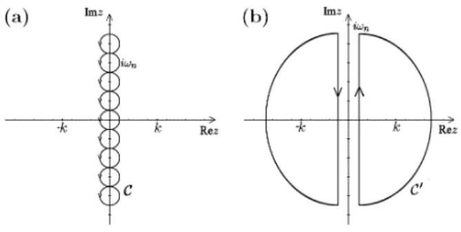
eβz−1, (3) and the integration contourC is defined in Fig. 1-(a).
The functionf(z) has poles atz=±k, being there-fore outside the contourC. Those ofδBE(βz), are sit-uated atz=i2πn/β=iωn, (n= 0,±1,±2, . . .) hence inside the contourC.
It is easy to see, using the residue theorem [7] that the sum coincides with the integral IC and, therefore,
we have
IC = ∞ ∑
n=−∞
Res [f(iωn)δBE(β(iωn))]
= 1 β
∞ ∑
n=−∞
e−iωnτ
k2+ω2 n .
(4)
Figure 1 - Integration contour in the complex plane used in (a) Eq. (4) and (b) Eq. (5).
Deforming the contourCintoC′shown in Fig. 1-(b)
we have, using the residue theorem again:
IC′ =−(Res [f(−k)δBE(β(−k))] + Res [f(k)δBE(βk)])
= cosh
[
k(τ−β2)]
2ksinh[k(β2)] .
(5)
Hence, sinceIC =IC′, we have
1 β
∞ ∑
n=−∞
e−iωnτ
k2+ω2 n
=
cosh[k(τ−β2)]
2k sinh[k(β2)]
, (6)
which allows us to rewrite the expression (1) forGT(r)
as
GT(r) = 1
4π
∫ ∞
−∞
dk
e−ikxcosh[k(τ−β 2
)]
ksinh[k(β2)] . (7)
Observe that only the real part of the integral is non-vanishing. Making the change of variablek→(2π/β)y, defininga≡(2π/β)x,θ≡[(2π/β)τ−π], and introduc-ing the regulatorbwe may rewrite Eq. (7) as
GT(r) = lim b→0
1 2π
∫ ∞
0
dy ycosay coshθy
(y2+b2) sinhπy. (8)
This integral, which can be found in Ref. [8], gives
GT(r) = lim b→0
{
e−|a|bcosbθ 4 sinbπ +
∞ ∑
k=1
(−1)kke−|a|kcoskθ 2π(k2−b2)
}
.
(9) The sum above may be evaluated in terms of hy-pergeometric functions2F1with the help of
Obtaining a closed-form representation for the dual bosonic thermal Green function 3305-3
GT(r) = lim b→0
{e−|a|bcosbθ
4 sinbπ +
e−|a|−iθ 8π(b2−1)
[
b2F1
(
1−b,1,2−b;−e−|a|−iθ)
+2F1
(
1−b,1,2−b;−e−|a|−iθ)+be2iθ2F1
(
1−b,1,2−b;−e−|a|+iθ)
+e2iθ 2F1
(
1−b,1,2−b;−e−|a|+iθ)−b 2F1
(
b+ 1,1, b+ 2;−e−|a|−iθ)
+2F1
(
b+ 1,1, b+ 2;−e−|a|−iθ)−be2iθ 2F1
(
b+ 1,1, b+ 2;−e−|a|+iθ)
+e2iθ2F1
(
b+ 1,1, b+ 2;−e−|a|+iθ)]}.
(10)
Taking theb→0 limit in the expression above, we obtain (since2F1(1,1,2;−z) = ln(1+z z))
GT(r;b) = 1
4πb −
|a|
4π− 1
4πln
[(
1 +e−|a|−iθ) (1 +e−|a|+iθ)]. (11)
By inserting the expressions foraandθand defining the regulator mass µ0 ≡ (2π/β)e−1/2b, we may write
the scalar thermal Green function, after some algebra, as
GT(r) = lim µ0→0
− 1
4πln
{µ2 0β2
π2 [ cosh (2π β x ) − cos (2π β τ )]} , (12)
which coincides with the result presented for the first time in Ref. [2].
Finally, notice that the Eq. (12) may be also written as
GT(r) = lim µ0→0
− 1
4πln
[
µ20ζ(r)ζ∗(r)
]
, (13)
where (z=x+iτ)
ζ(r)≡ζ(z) = βπsinh
(π
βz
)
. (14)
3.
The dual thermal Green function
From Eq. (13) we can also see that the thermal Green function may be written as the real part of an analytic function of a complex variableζ, namely
GT(r;µ0) = Re [F(ζ)] =
1
2[F(ζ) +F
∗(ζ)], (15)
where F(ζ)≡ −(1/2π) ln [µ0ζ(r)].
The imaginary part ofF(ζ) may be written as
˜
GT(r)≡Im [F(ζ)] = 1
2i[F(ζ)− F
∗(ζ)]
=− 1
4πiln
[
ζ(r)
ζ∗(
r)
]
.
(16)
Now, from the analyticity of F(ζ), then, it fol-lows that its imaginary and real parts must satisfy the Cauchy-Riemann conditions, which are given by
ϵµν∂
νGT =−∂µG˜T, ϵµν∂νG˜T =∂µGT. (17)
This property characterizes ˜GT as the dual thermal Green function.
4.
Concluding remarks
We would like to make a few comments about Eq. (13). Firstly, we note that in the zero temperature limit (T → 0,β → ∞), we haveζ(z) → z and ζ∗(z) →z∗
and, therefore, we recover the well-known Green func-tion at zero temperature, namely
lim
β→∞GT(r;µ0) =−
1 4πln
[
µ20zz∗
]
=− 1
4πln
[
µ20||r||2
]
.
(18) Comparing Eq. (13) with Eq. (18) we can also see that the only effect of introducing a finite temperature is to exchange the complex variable z for ζ(z). Since ζ(z) is analytic, we conclude that the thermal Green function is obtained from the one at zero temperature by the following conformal mapping [7]: the infinite strip 0< τ < β and−∞< x <∞is mapped into the region within the upper-half-ζ-plane. Notice that only the values [0, β] of τ are relevant because this variable is periodic inβ, as it should at finiteT.
Acknowledgments
The author would like to thank E.C. Marino for his valuable comments during the calculations.
This work has been supported in part by Funda¸c˜ao CECIERJ.
References
[1] H.A. Weldon, Phys. Rev. D 62, 056003 (2000); H.A. Weldon, Phys. Rev. D62, 056010 (2000).
[2] D. Del´epine, R. Gonz´alez Felipe, and J. Weyers, Phys. Lett. B419, 296 (1998).
3305-4 Mondaini
[4] A. Das, Finite Temperature Field Theory (World Sci-entific, Singapore, 1997).
[5] L. Mondaini and E.C. Marino, Mod. Phys. Lett. A23, 761 (2008).
[6] A.L. Fetter and J.D. Walecka, Quantum Theory of Many-Particle Systems (Dover Publications, Inc., New York, 2003).
[7] H.J. Weber and G.B. Arfken,Essential Mathematical
Methods for Physicists (Elsevier Academic Press, San Diego, 2004).
[8] I.S. Gradshteyn and I.M. Ryzhik, Table of Integrals, Series, and Products (Academic Press, San Diego, 2000).