Particle Emission in Hydrodynamics: a Problem Needing a Solution
F. Grassi
Instituto de F´ısica, Universidade de S˜ao Paulo, C. P. 66318, 05315-970 S˜ao Paulo-SP, Brazil
Received on 15 December, 2004
A survey of various mechanisms for particle emission in hydrodynamics is presented. First, in the case of sud-den freeze out, the problem of negative contributions in the Cooper-Frye formula and ways out are presented. Then the separate chemical and thermal freeze out scenario is described and the necessity of its inclusion in a hydrodynamical code is discussed. Finally, we show how to formulate continuous particle emission in hydro-dynamics and discuss extensively its consistency with data. We point out in various cases that the interpretation of data is quite influenced by the choice of the particle emission mechanism.
1
Introduction
Historically, the hydrodynamical model was suggested in 1953 by Landau [1] as a way to improve Fermi statistical model [2]. For decades, hydrodynamics was used to de-scribe collisions involving elementary particles and nuclei. But it really got wider acceptation with the advent of rel-ativistic (truly) heavy ion collisions, due to the large num-ber of particles created and its success in reproducing data. Brazil has a good tradition with hydrodynamics. Many as-pects of it have been treated by various persons. For illus-tration, the following papers can be quoted. Initial condi-tions were studied in [3, 4]. Solucondi-tions of the hydrodynamical equations using symmetries [5, 6] or numerical [7, 8] were investigated. The equation of dense matter was derived in [9, 10]. Comparison with data was performed in [11-17]. The emission mechanism was considered in [18-23]. In this paper, I concentrate on the problem of particle emission in hydrodynamics. In the Fermi description, energy is stored in a small volume, particles are produced according to the laws of statistical equilibrium at the instant of equilibrium and they immediately stop interacting, i.e. they freeze out. Landau took up these ideas: energy is stored in a small vol-ume, particles are produced according to the laws of sta-tistical equilibrium at the instant of equilibrium, expansion occurs (modifying particle numbers in agreement with the laws of conservation) and stops when the mean free path be-comes of order the linear dimension of the system, which led to a decoupling temperature of order the pion mass for a certain energy and slowly decreasing with increasing en-ergy. In today’s hydrodynamical description, two Lorentz contracted nuclei collide. Complex processes take place in the initial stage leading to a state of thermalized hot dense matter at some proper timeτ0. This matter evolves
accord-ing to the laws of hydrodynamics. As the expansion pro-ceeds, the fluid becomes cooler and more diluted until inter-actions stop and particles free-stream towards the detectors. In the following, I review various possible descriptions for this last stage of the hydrodynamical description. The usual
mechanism for particle emission in hydrodynamics is sud-den freeze out so I will use it as a point of comparison. I will start in section 2, reminding what it is, some of its problems and ways outs. There is another particle emission scenario which is a small extension of this idea of sudden freeze out: the separate chemical and thermal freeze out scenario. It has become used a lot e.g. to analyse data. So I will discuss in section 3 what it is, its alternatives and how to incorporate it in hydrodynamics. Continuous emission is a mechanism for particle emission that we proposed some years ago. As the very name suggests, it is not “sudden” like the usual freeze out mechanism. I will explain what it is precisely in section 4 and how it describes data compared to freeze out. Finally I will conclude in section 5.
2
Sudden freeze out
2.1
The traditional approach and its
prob-lems
Traditionally in hydrodynamics, the following simple pic-ture is used. Matter expands until a certain dilution criterion is satisfied. Often the criterion used is that a certain tem-perature has been reached, typically around 140 MeV in the spirit of Landau’s case. In some more modern version such as [24], a certain freeze out density must be reached. There also exist attempts [19,25-28] to incorporate more physical informations about the freeze out, for example type i parti-cles stop interacting when their average time between inter-actionsτi
scattbecomes greater than the fluid expansion time and average time to reach the border. When the freeze out criterion is reached, it is assumed that all particles stop in-teracting suddenly (this is called “freeze out”) and fly freely towards the detectors. As a consequence, observables only reflect the conditions (temperature, chemical potential, fluid velocity) met by matter late in its evolution.
Cooper-Frye formula (1) [29] may be used.
Ed3N
dp3 =
Tf.out
dσµpµf(x, p). (1) dσµis the normal vector to this surface,pµthe particle mo-mentum and f its distribution function. Usually one as-sumes a Bose-Einstein or Fermi-Dirac distribution for this
f.
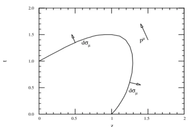
This sudden freeze out approach is often used however it is known to have some bad features. I will mention two. First when using the Cooper-Frye formula, we sometime meet negative terms (dσµpµ ≤ 0) corresponding to parti-cles re-entering the fluid. However since they presumably had stopped interacting (being in the frozen out region), they should not re-enter the fluid and start interacting again.
t
z
0 0.5 1 1.5 2
0.0 0.5 1.0 1.5 2.0
dσµ
dσµ pµ
Figure 1. In Cooper-Frye formula, the expressionpµdσµmay be negative.
-5 -4 -3 -2 -1 0 1 2 3 4 5
y
0.0 0.02 0.04 0.06 0.08 0.1
(1/V
0
T0
3 )
dN/dy
Tf=0.4 T0
spacelike timelike sum
Figure 2. Rapidity distribution of particles freezing out on the
Tf.out= 0.4T0isotherm in the Landau model. The solid line
cor-responds to all the contributions in formula 1, the dashed-dotted line represents contributions from space-like parts of the isotherm and the dashed line contributions from time-like parts [33, 34]. In this last case, note the negative contributions at y=0.
So usually one removes these negative terms from the calculations as being unphysical. However by doing this, one removes baryon number, energy and momentum from the calculation and violates conservation laws. It is not a negligible problem, as shown in the Fig. 2. In the code SPHERIO [8], it can be a 20% overestimate of particle num-ber. There are some ways to avoid these violations but none is completely satisfying [21].
The second problem is the following: do particles really
suddenlystop interacting when they reach a certain hyper-surface? Intuitively no, this must happen over a mean free path. This is corroborated by results from simulations of microscopical models[30, 31, 32]: the shape of the region where particles last interacted is generally not a sharp sur-face as assumed for sudden freeze outs. Some exceptions might be heavy particles in heavy systems or the phase tran-sition hypersurface.
We postpone the discussion of the second problem to section 4 and turn to the first problem.
2.2
Improved freeze out
In this section, we adopt the sudden freeze out picture and seek ways to incorporate conservation laws [21].
We suppose that prior to crossing the freeze out surface
σ, particles have a thermalized distribution function and we know the baryonic current and energy momentum tensor,nµ0
andT0µν. We suppose also that after crossing the surface, the distribution function is
f∗
F O(x, p;dσµ) =fF O(x, p)Θ(pµdσµ) (2) TheΘ function selects among particles which are emitted only only those withdσµpµ >0. This equation is solved in the rest frame of the gas doing freeze out (RFG) in Fig. 3. We see that according to the value ofv = dσ0/dσxRF G, a
region more or less big in thep⊥−pxspace can be excluded.
−2 −1.5 −1 −0.5 0 0.5 1 1.5 2 −2
−1.5 −1 −0.5 0 0.5 1 1.5 2
px[mc]
p⊥
[mc]
We do not know what the shape offF O(x, p)is. To sim-plify, we first suppose that
fF O(x, p) = 1 (2π)3exp
−p
µuµ+µ T
(3)
withuµ=γ(1, v,0,0)andµis the baryonic potential. This does not mean thatfF O is thermalized but simply that we choose a parametrization of the thermalized type. This parametrization is arbitrary, we discuss later how to improve our ansatz. For the moment we use it to illustrate how to pro-ceed in order not to violate conservation laws when using the Cooper-Frye formula.
It is possible to find expressions for the baryonic current, energy momentum tensor and entropy current corresponding to 2 in terms of Bessel-like functions and for massless par-ticules, even analytical expressions as function ofv,T eµ
[21].
To determine the parametersv,T andµfor matter on the post-freeze out side ofσ, we need to solve the conservation equations
[Nµdσµ] = 0 [T0µdσµ] = 0 [Txµdσµ] = 0, as function of quantities for matter on the pre-freeze out side,v0,T0eµ0. This being done, we still need to check
that
[Sµdσ
µ]≥0orR= S µdσ
µ Sµ
0dσµ ≥1
i.e. entropy can only increase when crossingσ. Generally, these equations need to be solved numerically but for mass-less particles, they have an analytical solution [21]. For il-lustration, we show this solution for the case of a plasma with an MIT bag equation of state in Fig. 4. An interesting result can be seen on the top figure. Normally when using a Cooper-Frye formula, the velocity of matter pre and post freeze out is assumed to be the same. However in the fig-ure, one sees that when imposing conservation laws, matter may be acelerated in a subtantial way. For example in case a),v0 = 0.2impliesvf low = 0.4andv = 0.6. In term of effective temperature, there was an increase of 60%.
This example illustrates the importance of taking into account conservation laws when crossingσ. However, the choice of fF O as being parametrized in the same way as a thermalized distribution is arbitrary as we mentioned al-ready. So we now study a more physical way of computing this function.
Consider an infinite tube with thex <0part filled with matter and the x > 0 part empty. At t=0, we remove the partition atx= 0and matter expands in vacuum. Suppose we remove the particles on the right hand side and put them back on the left hand side continuously so as to get a station-ary flow, with a rarefaction wave propagating to the left of the matter.
In the spirit of the continuous emission model presented below, the distribution function of matter has two compo-nents, ff ree andfint. Suppose thatff ree(x = 0, p) = 0 andfint(x= 0, p) = ftherm((x= 0, p). A simple model for the fluid evolution is
a b c
1 0.1 0.2 0.3 0.4 0.5 0.6 0.7 0.8 0.9 −1
−0.8 −0.6 −0.4 −0.2 0 0.2 0.4 0.6 0.8 1
v0
v,v
flow
0.1 0.2 0.3 0.4 0.5 0.6 0.7 0.8 0.9 0.1
0.2 0.3 0.4 0.5 0.6 0.7 0.8 0.9
n0[1/fm3]
n[1/fm
3 ]
30 40 50 60 70 80 90 10 1
1.5 2 2.5
R
T0 [MeV]
Figure 4. Solution of conservation laws in the case of a plasma. Top:vas function ofv0(solid line) for a)n0= 1.2f m−3, T0= 60M eV,ΛB ≡ B1/4 = 225M eV, b)n0 = 0.1f m−3, T0 =
60M eV,ΛB = 80M eV, c) n0 = 1.2f m−3, T0 =
60M eV,ΛB = 0M eV. (Dashed lines: velocity of pos-freeze
out baryonic flow).
Middle: baryonic density n as function of n0 for v0 = 0.5, T0 = 50M eV, a)ΛB = 80M eV (continuous line), b)ΛB = 120M eV (dashed-dotted line), c)ΛB = 160M eV (dashed line).
Bottom :R, ratio of entropy currents for post and pre-freeze matter as function ofT0for a)n0 = 0.1f m−
3
, v0 = 0.5M eV,ΛB = 80M eV (solid line), b)n0 = 0.5f m−
3
, v0= 0.5M eV,ΛB = 80M eV (dashed line), c)n0= 1.2f m−
3
∂xfint(x, p)dx = −Θ(pµdˆσµ) cosθp
λ fint(x, p)dx,
∂xff ree(x, p)dx = +Θ(pµdˆσµ) cosθp
λ fint(x, p)dx.
(4) wherecosθP =ppxin the rest frame of the rarefaction wave. A solution for these equations is
fint(x, p) =ftherm(x= 0, p) exp
−Θ(pµdˆσµ) cosθp
λ x
.
(5) and
ff ree(x, p) = ftherm(x= 0, p)×
1−exp
−Θ(pµdˆσµ)cosθp
λ x
= ftherm(x= 0, p)−fint(x, p) (6) We see that ff ree tends to the cut thermalized distribution we saw above whenx −→ ∞. In this model, the particle density does not change withxbut particles withpµdˆσ
µ>0 pass gradually fromfinttoff ree.
To improve this model, we consider
∂xfint(x, p)dx = −Θ(pµdˆσµ) cosθp
λ fint(x, p)dx
+ [feq(x, p)−fint(x, p)] 1 λ′dx,
(7)
∂xff ree(x, p)dx= +Θ(pµdˆσµ) cosθp
λ fint(x, p)dx. (8)
The additional term in fint includes the tendency for this function to tend towards an equilibrium function due to col-lisions with a relaxation distanceλ′. Due to the loss of
en-ergy, momentum and particle number, feq is not the initial thermalized function but its parametersneq(x),Teq(x)and uµ
eq(x)can be determined using conservation laws. In the case of immediate re-thermalization (fint =feq), for a gas of massless particles with zero net baryon number, the solu-tion is shown in Fig. 5. One sees that the solusolu-tionff ree is not a thermalized type cut function.
Even more importantly, this distribution exibits a curva-ture which reminds the data on p⊥ distribution for pions.
Other explaination for this curvature are transverse expan-sion or resonance decays. On the basis of our work, it is dif-ficult to trust totally analyses which extracts thermal freeze out temperatures and fluid velocities using only transverse expansion and resonance decays.
More details and improvement on how to compute the post freeze out distribution function were presented in vari-ous papers [35-39].
Finally, it is interesting to note that models that com-bine hydrodynamics with a cascade code also suffer from the problem of non-conservation of energy-momentum and charge [40] or inconsistency [41], as discussed in [42].
0 0.5 1 1.5
10−6
10−5
10−4
10−3
10−2
10−1
P [GeV]x
f(
p
)
[ar
b
. un
its
]
V0= 0.5 V0= 0 V0 = −0.5
Figure 5.ff ree(px)(equivalent to thefF O∗ in the previous section),
computed atpy= 0, x= 100λ, T0= 130M eV.
3
Separate freeze outs
In this section, we suppose that the sudden freeze out picture can be used and see how well it describes data.
3.1
Chemical freeze out
Strangeness production plays a special part in ultrarelativis-tic nuclear collisions since its increase might be evidence for the creation of quark gluon plasma. Many experiments therefore collect information on strangeness production.
We can consider for example the results obtained by the CERN collaborations WA85 (collision S+W), WA 94 (colli-sion S+S) and WA97, later on NA57 (colli(colli-sion Pb+Pb). One can combine various ratios to obtain a window for the freeze out conditions compatible with all these data. The basic idea is simple, for example:
Λ/Λ∼exp2(µS −µB)
T |f.out=exp. value. (9) (neglecting decays.)
In principle, this equation depends on three variables. However, supposing that strangeness is locally conserved, this leads to a relation µS(µb, T), then given a minimum and a maximum values, the above equation gives a relation
Figure 6. Search of a window [44] of values ofTf.outeµb, f.outreproducing WA85 data. This window only exists forγ < 1(for this reference).
The parameterγin this figure is basically a phenomeno-logical factor, which indicates how far from chemical equi-librium we are, it is introduced in front of the factorse±µs/T whereµsis the s quark chemical potential,µs=µB/3−µS. (There exists a study by C.Slotta et al. [43] motivating this way of includingγ.) It can be seen that ifγ = 0,7 it is possible to reproduce the experimental ratiosΛ/Λ, Ξ/Ξ,
Ξ/Λ, Ξ/Λ choosing Tf.out and µb, f.out in a certain win-dow. This window is located aroundTf.out ∼ 180−200 MeV,µb, f.out ∼200−300MeV. One can be surprised by such high values since particle densities are still high. How-ever these results are rather typical as can be checked in the table 1.
TABLE 1. Summary of freeze out values from J.Sollfrank [45]. collision T (MeV) µb(MeV) γs ref.
S+S 170 257 1 [46]
197±29 267±21 1.00±0.21 [47]
185 301 1 [48]
192±15 222±10 1 [49]
182±9 226±13 0.73±0.04 [50]
202±13 259±15 0.84±0.07 [51]
S+Ag 191±17 279±33 1 [49]
180.0±3.2 238±12 0.83±0.07 [50]
185±8 244±14 0.82±0.07 [51]
S+Pb 172±16 292±42 1 [52]
S+W 190±10 240±40 0.7 [44]
190 223±19 0.68±0.06 [53]
196±9 231±18 1 [54]
S+Au(W,Pb) 165±5 175±5 1 [49]
160 171 1 [55]
160.2±3.5 158±4 0.66±0.04 [51] The explaination usually given nowadays is that at these temperatures, particles are doing achemical freeze out, they stop having inelastic collisions and their abundances are frozen.
3.2
Thermal freeze out
Transverse mass distributions obtained experimentally (when plotted logarithmically) exhibit large inverse
inclina-tions. These are called effective temperatures.
In the case of hydrodynamics, these effective tempera-tures are thought to be due to the convolution of the fluid temperature with its transverse velocity, both at freeze out. So in particular the effective temperatures are higher than the fluid temperature. In addition, the effective temperature should be larger the larger the particle mass is , since the “kick” received in momentum, ∼ mvf luidf.out, due to trans-verse expansion, is larger (this argument is only valid for the non-relativistic part of the spectrum i.e. p⊥ << m; the
effective temperature does not depend on mass for the part of the spectrum where p⊥ >> m(but for that part of the
spectra other phenomena might be important). In general, given an experimentalm⊥spectrum, there exist many pairs
ofTf.outandvf luidf.out which can reproduce it.
To remove this ambiguity, we can compare them⊥
spec-tra for various types of particles (e.g. [56]), or for a given type of particle, for example pions, combine the fit of the spectrum with results on HBT correlations (e.g. [57]). A compilation for various accelerator energies of values for
Figure 7. Phase diagram with lines indicating values of freeze out parameters at various energies obtained from particle abundances (solid line) and particle spectra (dashed line) [58].
3.3
Is it quantitatively necessary to modify
hydrodynamics to incorporate separate
freeze outs?
In [22], we made a preliminary study of whether such a sep-arate freeze out model would quantitatively influence the hy-drodynamical expansion of the fluid. For this, we used a simple hydrodynamical model, with longitudinal expansion only and longitudinal boost invariance [59].
For a single freeze out, the hydrodynamical equations are
∂ǫ
∂t+
ǫ+p
t = 0
∂nB
∂t +
nB
t = 0 (10)
The last equation can be solved easily
nB(t) =
nB(t0)t0
t . (11)
Given an equation of state,p(ǫ, nB), we can getǫ(t)and nB(t), solving (10). From them,T(t)andµB(t)can be ex-tracted. So, if the freeze out criterion isTf.out=constant, one can see which are the values for other quantities at freeze out, for example the values oftf.out,µB f.out, ... These val-ues being known, spectra can be computed.
Now let us start again with the previous model, but we suppose that when a certain temperatureTch.f.outis reached (corresponding to a certaintch.f.out) some abundances are frozen. To fix ideas, let us suppose thatΛandΛ¯ are in this situation. In this case, fort≥tch.f.out, in addition to the hy-drodynamic equations above, ( 10), we must introduce sep-arate conservation laws for these two types of particles
∂nΛ
∂t +
nΛ
t = 0 (12)
∂nΛ¯
∂t +
nΛ¯
t = 0. (13)
Again it is easy to solve these equations
nΛ(t) = nΛ(t0)t0
t (14)
nΛ¯(t) = nΛ¯(t0)t0
t (15)
For timest≥tch.f.out, we need to solve the hydrodynamic equations ( 10) with an equation of state modified to incor-porate these conserved abundances.
We suppose that the fluid is a gas of non-interacting res-onances.
ni =
gim2iT 2π2
∞
n=1
(∓)n+1enµi/T
n K2(nmi/T) (16)
ǫi = gim
2
iT2 2π2
∞
n=1
(∓)n+1e nµi/T
n2 [3K2(nmi/T)
+ nmi
T K1(nmi/T)] (17)
pi =
gim2iT2 2π2
∞
n=1
(∓)n+1e nµi/T
n2 K2(nmi/T) (18)
wheremiis the particle mass,gi, its degeneracy andµi, its chemical potential, the minus sign holds for fermions and plus for bosons. In principle each particle speciesi mak-ing early chemical freeze-out has a chemical potential as-sociated to it; this potential controls the conservation of the number of particles of typei. For particle species not mak-ing early chemical freeze-out, the chemical potential is of the usual type,µi = BiµB +SiµS, where µB (µS) en-sures the conservation of baryon number (strangeness) and
Bi (Si) is the baryon (strangeness) number of particle of typei. So the modified equation of state depends not only onTandµBbut alsoµΛ,µΛ¯, etc. (the notation “etc” stands
for all the other particles making early chemical freeze-out). This complicates the hydrodynamical problem, however we can note the following.
Ifmi−µi >> T (the density of typeiparticle is low) andmi >> T, (these relations should hold for all particles except pions and we checked them for various times and particle types) the following approximations can be used
ni =
gi 2π2
π 2(miT)
3/2e(µi−mi)/T
×
1 + 15T 8mi
+ 105T 2
128m2
i +...
(19)
ǫi = nimi
1 + 3T 2mi
+15T 2
8m2
i +...
(20)
pi = niT (21)
We note thatǫiandpiare written in term ofniand T. There-fore we can work with the variables T, µB, nΛ, nΛ¯, etc,
rather than T, µB, µΛ, µΛ¯, etc. The time dependence of nΛ, nΛ¯, etcis known as discussed already. So the modified
Figure 8. µB and T as function of time in the case where all
particles have simultaneous freeze-outs (dashed line) and (I) all strange particles in basic multiplets make an early chemical freeze-out (continuous line), (II) all strange particles exceptKandK∗’s make an early chemical freeze-out (dotted line).
In Fig. 8, we compare the behavior ofTandµBas func-tion oft, obtained from the hydrodynamical equations using the modified equation of state and the unmodified one. We see that if the chemical and thermal freeze-out temperatures are very different or if many particle species make an early chemical freeze out, the thermal freeze out time is quite af-fected. Therefore it is important to take into account the effect of the early chemical freeze-out on the equation of state to make predictions for observables which depend on thermal freeze-out volumes (which are related to the ther-mal freeze out time), for example particle abundances and eventually particle correlations.
If the chemical and thermal freeze-out temperatures are not very different or if few particle species make the early freeze out, one can proceed as follows. One can use an un-modified equation of state in a hydrodynamical code and to account for early chemical freeze-out of speciesi, when the number of typeiparticles was fixed, use a modified Cooper-Frye formula
Ed3N
i
dp3 =
Ni(Tch.f.)
Ni(Tth.f.)
×
Sth.f.
dσµpµf(x, p). (22)
The second factor on the right hand side is the usual one and it gives the shape of the spectrum at thermal freeze-out, the first factor is a normalizing term introduced such that upon integration on momentump, the number of particles of type
iisNi(Tch.f). As an illustration, using HYLANDER-PLUS [60], we show in Fig. 9 that both the shapes ofm⊥spectra
and abundances can be reproduced forTch.f. = 176MeV and Tth.f. = 139 MeV, while simultaneous freeze-outs at
Tch.f. =Tth.f. = 139MeV would yield the correct shapes but too few particles.
0 0.5 1 1.5 2
mt−m Λ [GeV]
10−2 10−1
100 101 102
1/m
t
dN/dm
t
[GeV
−2
]
Λ
Tch=184MeV
Tch=176MeV
Tch=Tth=139MeV
FIGURE 1
0 0.5 1 1.5 2
mt−m Λ [GeV]
10−2
10−1 100 101 102
1/m
t
dN/dm
t
[GeV
−2 ]
Λ
Tch=184MeV
Tch=176MeV
Tch=Tth=139MeV
FIGURE 2
1 1.5 2 2.5 3
mt[GeV] 10−3
10−2 10−1 100
101
1/m
t
dN/dm
t
1/dy [GeV
−2 ]
Ξ
Tch=184MeV
Tch=176MeV
Tch=Tth=139MeV
FIGURE 3
1 1.5 2 2.5 3
mt[GeV] 10−3
10−2 10−1 100
101
1/m
t
dN/dm
t
1/dy [GeV
−2]
Ξ
Tch=184MeV
Tch=176MeV
Tch=Tth=139MeV
FIGURE 4
Figure 9.m⊥spectra: NA49 data and HYLANDER-PLUS results.
Hirano and Tsuda [24] confirmed the importance of in-cluding separate freeze outs in hydrodynamical codes, in particular they studied elliptic flow and HBT radii at RHIC. This is also consistent with results in [61].
4
Continuous emission
4.1
Formalism and modified fluid evolution
In this section, we present a possible way out of the second problem mentioned above. In colaboration with Y.Hama and T.Kodama, I made a description of particle emission [62, 63] which incorporates the fact that they, at each in-stant and each location, have a certain probability to escape without collision from the dense medium (said in the same terms as above: there exists a region in spacetime for the last collisions of each particle). So the distribution function of the system in expansion has two termsff ree, represent-ing particles that made their last collision already, andfint, corresponding to the particles that are still interacting
f(x, p) =ff ree(x, p) +fint(x, p) (23) The formula for the free particle spectra is given by
Ed3N/dp3=
d4x Dµ[pµff ree(x, p)] (24) (neglecting particles that are initially free; note that if it were not the case, the use of hydrodynamics would not be possi-ble).Dµindicates a four-divergence in general coordinates. This integral must be evaluated for the whole spacetime oc-cupied by the fluid.
This way, we see that the spectra contains information about the whole fluid history and not just the time when it is very diluted. (This formula reduces to the Cooper-Frye formula (1) in an adequate limit).
We can write
ff ree=Pf =P/(1− P)fint. (25) P(x, p) = ff ree/f, the fraction of free particles, can be identified with the probability that a particle of momentump
escapes fromxwithout collisions, so to compute this quan-tity we use the Glauber formula
P(x, p) =exp
−
∞
t
n(x′)σv
reldt′
. (26)
We suppose also that all interacting particles are ther-malized, so
fint(x, p) = fth(x, p) =g/(2π)3
× 1/{exp[(p.u(x)−µ(x))/T(x)]±1},
(27) whereuµis the fluid velocity,µits chemical potential (µ= µBB+µSSwithBthe baryonic number of the hadron,S, its strangeness andµBandµS the associated chemical po-tentials) andTits temperature atx.
To computeuµ,µandT, we must solve the equations of conservation of energy-momentum and baryonic number
DµTµ ν = 0 (28)
Dµ(nbuµ) = 0. (29)
In the Fig. 10, examples of solution are given. We can see that the fluid evolution with continuous emission is different from the usual case without continuous emis-sion. For example, and as expected, the temperature de-creases faster since free particles carry with them part of the energy-momentum.
In principle we have all the ingredients to compute (24). However there exist two problems: 1) numerically, in the equation 25 we can have divergencies ifP goes faster to 1 thanfintgoes to zero 2) the hypothesis thatfintis termal-ized (cf. eq.(27)) must loose its validity whenP goes to 1. To avoid this problem, we divide space-time in eq. (24), in two regions: the first withP > PF and the second with P ≤ PF, for some reasonable value ofPF. Using Gauss
theorem, the second part reduces to an integral over the sur-faceP =PF(which depends on the particle momentum)
I1 =
P=PF
dσµpµff ree (30)
= PF
1− PF
P=PF
dσµpµfth (31)
There is still a certain fraction of interacting particles,1− PFof the total, on this surface, it is these particles which in
principle turn free in the regionP >PF. To count them, we
suppose that they are rather diluted (i.e.PFis rather large)
and we can apply a Cooper-Frye formula for them
I2 ∼
P=PF
dσµpµfint (32)
=
P=PF
dσµpµfth (33)
So finally
Ed
3N
dp3 =I1+I2∼ 1 1− PF
P=PF
dσµpµfth. (34)
It is this formula which is used below, withPF = 0.5(but
we tested the effect of changing this value) and coordinates adequate for the geometry of the problem. It is similar to a Cooper-Frye formula (1), however one must note that the conditionP =PF depends not only on the localization of
a particle but its momentum, which as we will see has inter-esting consequences.
4.2
Comparison of the continuous emission
and freeze out scenarios
ρ
(fm)
T(GeV)
0.04 0.06 0.08 0.1 0.12 0.14 0.16 0.18 0.2
0 0.5 1 1.5 2 2.5 3 3.5 4
ρ
(fm)
µ
B(GeV)
0.2 0.3 0.4 0.5 0.6 0.7 0.8
0 0.5 1 1.5 2 2.5 3 3.5 4
5 10 15 20 r
0.05 0.1 0.15 0.2 Temperature
5 10 15 20 r
0.3 0.4 0.5 0.6 0.7 ub
5 10 15 20 r
0.2 0.4 0.6 0.8 1 v/c
Figure 10. Fluid evolution supposing longitudinal boost invarience[59]. Top two: for a light projectile such as S,TandµB as function of radius; as a first approximation transverse expansion is neglected. (Solid lines correspond to a fluid with continuous emission, dashed line lines to a fluid without continuous emission, i.e. the usual case.) Bottom three: for a heavy projectile such as Pb,T,µBand fluid velocity as function of radius; transverse ex-pansion is included (times: 1,4,7,10 fm).
a. Strange particle ratios
We saw above that for the freeze out mechanism, strange particle ratios give information about chemical freeze out. Now we see how to interpret these data within the continu-ous emission sceanrio [64-68]. In this case, the only para-meters are the initial conditionsT0 eµb0 and a value that
we suppose average forγ. We therefore fix a set of them, solve the equations of hydrodinamics with continuous emis-sion, compute and integrate inp⊥the spectra given by (34)
for each type of particles (we include also the decays of the various types of particles in one another). In a way similar to freeze out but now with initial values instead of freeze out values, we get in Fig. 11, a window of initial conditions which permits to reproduce the various experimental ratios. (We also look at other ratios than those shown in the figure, tested the effect of changes in the equation of state, cross section, initial time, type of experimental cutoff.)
We see therefore that the initial conditions necessary to reproduce the WA85 data are
These values may seem high for the existence of a hadronic phase, lattice gauge QCD simulations seem to indicate val-ues smaller for the quark-hadron transition. Here we can note that 1) values of QCD on the lattice are still evolv-ing (problems exist to incorporate quarks with intermediate mass, include µb = 0, etc. 2) Our own model is still be-ing improved and we know for example that the equation of state affects the localization of the window in initial condi-tions compatible with data.
µ
B0(GeV)
T
0(GeV)
0.15 0.16 0.17 0.18 0.19 0.2 0.21 0.22 0.23 0.24 0.25
0.1 0.15 0.2 0.25 0.3 0.35 0.4
Figure 11. Window in initial conditions allowing to reproduce WA85 data, for an equation of state with excluded volume cor-rections [15].
0 .1 5 0 .2 0 0 .2 5 0 .3 0 0 .3 5 0 .4 0
µ
B 0
(G eV )
0 .1 6 0 .2 0 0 .2 4 0 .2 8 0 .3 2 0 .3 6
T 0
(G
e
V
)
Λ/Λ
Ξ/Ξ
Ξ/Λ Ξ/Λ
Figure 12. Window in initial conditions reproducing WA97 data in the case of an equation of state without excluded volume correc-tions. With volume corrections, the window is lower [17].
In Fig. 12, the same kind of analysis was done for the data WA97. With the reservation in the caption of the fig-ure, we see that the initial conditions are not very different from the one above.
We can therefore conclude that the interpretation of data on particle ratios lead to totally different information accord-ing to the emission model used. For the freeze out model, we get information about chemical freeze out while for con-tinuous emission, we learn about the initial conditions.
b. Transverse mass spectra
For freeze out, we saw that these spectra tell us about thermal freeze out (temperature and fluid velocity). Now for continuous emission let us see how to interpret these same spectra [64-68]. In this case, the initial conditions were al-ready determined from strange particle ratios, they cannot be changed and must be used to compute the spectra as well. For example, in Fig. 13, various spectra are shown, assum-ingT0=µb0= 200MeV, and compared with experimental
data.
This comparison should not be considered as a fit but as a test of the possibility of interpreting various types of data in a self-consistent way with continuous emission (in partic-ular note that our calculations were done assuming longitu-dinal boost invariance).
We learn various information from this comparison. In these figures, we do not take into account transverse expan-sion. With the S+S NA35 data, we note that the heavy par-ticles and high transverse momentum pions have similar in-verse inclinationsT0∼200MeV. The particles heavier than
pions, due to termal suppression, are mainly emitted early when the temperature is∼T0. For lower temperatures, there
are still emitted (and more easily due to matter dilution) but their densities are quite smaller (this is what is called thermal suppression) and their contributions as well. The high transverse momentum pions have large velocity and (if not too far away from the outer fluid surface) escape with-out collision earlier than pions at the same place but with smaller velocity, so these high transverse momentum pions also escape at∼T0. Pions are small mass particles and are
little affected by thermal suppression. This way, they can escape in significative number at various temperatures. This is reflected by their spectra, precisely its curvature. (In our calculation, decays into pions are not included, this would fill the small transverse momentum region and improve the agreement with experimental data.)
The S+S WA94 data also indicate that continuous emis-sion is compatible with data. Finally, the S+W WA85 data seem to indicate that perhaps somewhat different initial con-ditions or a little of transverse expansion might be necessary to reproduce data.
m⊥(GeV)
dN/dym
⊥
dm
⊥
(a.u.) π
- K o s P Λ
1 10 102 103 104
0.25 0.5 0.75 1 1.25 1.5 1.75 2 2.25 2.5
dN/dym
⊥
dm
⊥
(a.u.) Λ
Λ–
Ξ
m⊥(GeV)
Ξ–
102
103
104
105
106
107
108
109
1010
1.5 1.75 2 2.25 2.5 2.75 3 3.25 3.5
dN/dym
⊥
dm
⊥
(a.u.)
Λ
Λ–
K0s K+
m⊥(GeV) K
-103
104
105
106
107
108
109
1010
1 1.25 1.5 1.75 2 2.25 2.5 2.75 3
Figure 13. Using longitudinal boost invariance and no transverse expansion, we compare our predictions, top to bottom, with NA35 data (S+S, all rapidity), with WA94 data (S+S, midrapidity, large transverse momenta) and with WA85 data (S+W, midrapidity, large transverse momenta) [16].
0 .0 0 0 .4 0 0 .8 0 1 .2 0 1 .6 0 2 .0 0
m - m (G eV )
0 .0 1 0 .1 0 1 .0 0 1 0 .0 0 1 0 0 .0 0
dN
/(
d
y
dm
)
(a.
u
.)
P re lim in a ry
2
Figure 14. WA97 data and example of comparison with continu-ous emission with transverse expansion (not a least square fit) for
T0=µb.0= 200MeV [17].
Figure 15. Compilation of experimental data on effective temper-atures in the case of heavy projectile and predictions for usual hy-drodynamics [66]. (The various experiments have different rapid-ity and transverse momentum cutoffs). In general, deuteron is left outside the hydrodynamical analysis: it is little bounded and should form later in the fluid evolution from coalescence of a neutron and a proton with similar moment..
c. The case of theΩ
lower than other particles in Fig. 15 A possible explaination within hydrodynamics with separate freeze outs, is that the
Ωmade its chemical and thermal freeze out together, early. Van Hecke et al. [66] argued that this is reasonable since it is expected thatΩhas a small cross section (because there is no channel forΩπ→ resonance→ Ωπ) and showed that the microscopical model RQMD can reproduce the data.
In our model originally we had used the same value of the cross sections to compute the escape probability for the various types of particles. This is not expected and indeed in this case, continuous emission, does not lead to good pre-dictions as shown in Fig. 17a. Therefore in the spirit of mi-croscopic models, we also show our predictions in Fig. 17b, for continuous emission and the following cross sections:
σππ ∼< σvrel >ππ∼ 1f m2, σN π ∼< σvrel >N π∼ 3/2 < σvrel >ππ (using additive quark model estimate), σΛπ ∼< σvrel >Λπ∼ 1,2 < σvrel >ππ (using addi-tive quark model estimate [67]) andσΩπ ∼< σvrel >Ωπ∼ 1/2< σvrel>N π(using estimate in [68]). The predictions now are in agreement with data. However, the cross sec-tions are poorly known and our results are sensitive to their values.
Recently, with new data by NA49, WA97 [70] and NA49 [71] came to the conclusion that in fact there is no need for early joint chemical and thermal freeze outs for the
Ω: all their spectra can be fitted with a simple hydro in-spired model as seen in Fig. 18. The previous difficulty for WA97 came from the fact [72] thatΩwas observed at high
p⊥. However now, STAR has problems [73] to fit with a
simple hydro inspired model theΞtogether withπ, p, K,Λ
and would need to assume early joint chemical and thermal freeze outs for theΞ, as shown in Fig. 19. More recently, it has been noted [74] by NA49, that their conclusion depends on the parametrization used and in [75], NA57 argues that due to low statistics, it is not clear what conclusion can be drawn for theΩ. In [76], an attempt was made to reproduce with a single thermal freeze out temperature in a hydrody-namical code, all transverse mass spectra at a given energy.
Figure 16. Predictions from RQMD [66] in the same experimental situation as the previous figure.
❍ Dados Experimentais
★ Emissa~o Conti′nua
(a)
Massa da Parti′cula(GeV/c2)
Temperatura aparente (GeV)
175 200 225 250 275 300 325 350 375
0 0.2 0.4 0.6 0.8 1 1.2 1.4 1.6 1.8 2
❍ Dados Experimentais
★ Emissa~o Conti′nua
(b)
Massa da Parti′cula(GeV/c2)
Temperatura aparente (GeV)
175 200 225 250 275 300 325 350 375
0 0.2 0.4 0.6 0.8 1 1.2 1.4 1.6 1.8 2
Figure 17. Comparison of experimental data on effective temper-atures in the case of a heavy projectile with predictions from con-tinuous emission. Top: all cross section supposed equal. Bottom: more realistic cross section values (cf. text) [69, 17].
d. Pion abundances
We showed that strange particle ratios can be reproduced by a model with chemical freeze out around 180 MeV. The abundances too can be reproduced. The problem is that the pion number is too low. This was noticed by Davison et al. [77], as shown in their table 2 reproduced below
TABLE 2. Comparison between NA35 data and previsions from a thermal model[77].
KS0 K
+
K− Λ Λ “p’ π−
Th. 10.7 14.2 7.15 8.2 1.5 23.2 56.9 Exp. 10.7 12.5 6.9 8.2 1.5 22.0 92.7
Figure 18. Data and hydro inspired fit for all particles includingΩ, top, NA49 and bottom, NA57 [70, 71].
Figure 19. A hydro fit to transverse mass spectra leads to high
Tf.outforΞand lower forπ, p, K,Λ[73].
There are various ways to try to solve this problem. 1. It can be argued (in a spirit similar to Cleymans et al.
[78]) that strange particles do their chemical freeze our early around 180 MeV and their thermal freeze out around 140 MeV but the pions do their chemi-cal and thermal freeze outs together around 140 MeV. In fact Ster et al. [79] manage to reproduce data by NA49, NA44 and WA98 on spectra (including normalization i.e. abundances) for negatives, pions, kaons and protons and HBT radii (see next section) with temperature around 140 MeV and null chemical potential for the pions. On the other side, Tom´asik et al. [80] say that for the same kind of objective, they need temperatures of order 100 MeV and non zero chemical potential for the pions. So it is not clear if to reproduce the pion abundance, it is necessary to modify the hydrodynamics with separate freeze out, including pions out of chemical equilibrium or not. 2. Gorenstein and colaborators [81, 82, 83] studied
mod-ifications of the equation of state, precisely they in-cluded a smaller radius for the volume corrections of the pion.
3. Letessier et al. made a s´erie of papers [84, 53] argu-ing that the large pion abundance is indicative of the formation of a quark gluon plasma hadronizing sud-denly, with both strange and non-strange quarks out of chemical equilibrium [85].
Given the difficulty that freeze out models have with pi-ons, it is interesting to compute abundances with continuous emission models. In the table, results and NA35 data from S+S are shown (data are selected at midrapidity).
TABLE 3. Comparison between experimental data, results for con-tinuous emission atT0 = µb,0 = 200MeV and freeze out at T0=µb,0=Tf.out=µb f.out= 200MeV.
experimental continuous freeze out value emission
Λ 1.26±0.22 0.96 0.92
¯
Λ 0.44±0.16 0.29 0.46
p−p¯ 3.2±1.0 3.12 1.32
h− 26±1 27 15.7
K0
S 1.3±0.22 1.23 1.06
case, a large number of pions does not imply a large initial entropy and the existence of a plasma. It can be noted that the interpretation of data is quite influenced by the choice of the particle emission model.
e. HBT
Interferometry is a tool which permits extracting infor-mation on the spacetime structure of the particle emission source and is sensitive to the underlying dynamics. Since pion emission is different in freeze out and continuous emis-sion models, it is interesting to compare their interferometry predictions (for a review see [87]). This was done in ref. [88].
In this work, the formalism of continuous emission [62, 63] was extended to the computation of correlation functions. Precisely, we computed
C(k1, k2) =C(q, K) = 1 + |G(q, K)|
2
G(k1, k1)G(k2, k2)
, (36)
whereqµ=kµ
1−k
µ
2 eKµ=12(k
µ
1+k
µ
2).
In the case of freeze out (in the Bjorken model with pseudo-temperature[89])
G(k1, k2) = 2< dN
dy >{ 2
qTRTJ1(qTRT)}K0(ξ) (37) where
ξ2 = [ 1
2T(m1T +m2T)−iτ(m1T −m2T)]
2+
2 ( 1 4T2 +τ
2)m
1Tm2T[cosh(∆y)−1] ,(38) ∆y=y1−y2,< >indicates average over particles 1 and 2
and
G(ki, ki) = 2dN dyi
K0(miT
T ). (39)
In the case of continuous emission in the Bjorken model with pseudo-temperature
G(q, K) = 1
(2π)3(1− P F)
2π
0 dφ
+∞
−∞ dη
× {
RT
0
ρ dρ τFMT cosh(Y −η)
× ei[τF(q0coshη−qLsinhη)−ρqTcos(φ−φq)]
+
+∞
τ0
τ dτ ρFKTcosφ
× ei[τ(q0coshη−qLsinhη)−ρFqTcos(φ−φq)]}
× e−MTcosh(Y−η)/Tps(x),
(40) with MT =
K2
T +M2, KT = 12(k1 +k2)T, M2 = KµKµ = m2 − 14qµqµ, Y is the rapidity correspond-ing to K, φ is the azimuthal angle in relation to the di-rection of K and φq is the angle between the directions
of q andK. τPF andρPF are determined byP = PF.
Tps(x) = 1,42T(x)−12,7M eV.
In [88], a few idealized cases were studied and then some cases more representative of the experimental situa-tion, were presented. For example, instead ofC(q, K), we computed
C(qL) = 1 +
R180
−180dKL
R600 50 dKT
R30 0 dqS
R30
0 dqoC(K,q)|G(K,q)| 2
R180
−180dKL
R600 50 dKT
R30 0 dqS
R30
0 dqoC(K,q)G(k1,k1)G(k2,k2).
(41) (This corresponds to the experimental cuts of NA35). qO, qS eqLare defined in Fig. 20.
p2
p1
q = (q ,q ,q )o s
l
l = "long"
s = "side"
o = "out"
z x
y
K = (K ,0,K )l l
Figure 20. By definition : Oz is chosen along the beam andK
in thex−zplane. TheL(longitudinal) component of a vector is
itszcomponent, theO(“outward”) itsxcomponent andS (“side-wards”) itsycomponent [90].
In a first comparison, we used similar initial conditions than above,T0 = 200MeV (S+S collisions) for both
con-tinuous emission and freeze out. Results are presented as function ofqL,qOandqSin Fig. 21.
In a second comparison, given a curve obtained for con-tinuous emission, we try to find a similar curve obtained with the standard valueTf.out= 140MeV, varying the ini-tial temperatureT0f.out. The results are shown as function
ofqL,qO eqS in Fig. 22. From these two sets of figures, it can be seen that there are many differences in the correla-tions between both models: shape. heigth, etc. If the initial conditions are the same, the correlations are very different. Even more interesting if trying to approximate with a freeze out atTf.out = 140MeV, the continuous emission correla-tions, it is necessary to assume aT0 very high, where the
notion of hadronic gas looses its validity. So, we can see that if continuous emission is the correct description for ex-perimental data, it will be more difficult to attain the quark gluon plasma than it looks using the freeze out model. So again we conclude that what we learn about the hot dense matter created depends on the emission model used. (Note that to actually compare with data, transverse expansion has to be included.)
0 4 0 8 0 1 2 0 1 6 0 2 0 0 q
L(M e V ) 1 .0
1 .2 1 .4 1 .6 1 .8 2 .0
<
C
(K
,q
)>
C o ntinu ou s E m ission (T
0= 2 00 M e V ) F re eze -O ut (T
0= 2 00 M eV )
T
fo= 1 7 0 M e V T
fo= 1 4 0 M e V C .E .
0 4 0 8 0 1 2 0 1 6 0 2 0 0 q
o(M e V ) 1 .0
1 .2 1 .4 1 .6 1 .8 2 .0
<
C
(K
,q
)>
C o ntinu ou s E m ission (T
0= 2 00 M e V ) F re eze -O ut (T0= 2 00 M eV )
T
fo= 1 7 0 M e V T
fo= 1 4 0 M e V C .E .
0 4 0 8 0 1 2 0 1 6 0 2 0 0 q
s(M e V ) 1 .0
1 .2 1 .4 1 .6 1 .8 2 .0
<
C
(K
,q
)>
C o ntinu ou s E m ission (T0= 2 00 M e V ) F re eze -O ut (T0= 2 00 M eV )
T fo= 1 7 0 M e V T
fo= 1 4 0 M e V C .E .
Figure 21. Comparison of continuous emission with freeze out, when both have the same initial conditions [88].
f. Plasma
In all the previous analysis, we assumed that the fluid was initially composed of hadrons with some initial con-ditions T0,µb,0. Given the possibility that a quark gluon
plasma might have been created already, we must discuss the extension of our model to the case were a plasma might have been formed.
0 4 0 8 0 1 2 0 1 6 0 2 0 0 q
L(M e V ) 1 .0
1 .2 1 .4 1 .6 1 .8 2 .0
<
C
(K
,q
)>
C o ntinu ou s E m ission (T
0= 2 00 M e V ) F re eze -O ut (Tfo= 1 40 M eV )
T 0= 2 0 0 M e V T
0= 2 2 0 M e V T
0= 2 3 0 M e V C .E .
0 4 0 8 0 1 2 0 1 6 0 2 0 0
q o(M e V )
1 .0 1 .2 1 .4 1 .6 1 .8 2 .0
<
C
(K
,q
)>
C o ntinu ou s E m ission (T
0= 2 00 M e V ) F re eze -O ut (Tfo= 1 40 M eV )
T0= 2 0 0 M e V T0= 2 3 0 M e V T
0= 2 6 0 M e V C .E .
0 4 0 8 0 1 2 0 1 6 0 2 0 0
q s(M e V )
1 .0 1 .2 1 .4 1 .6 1 .8 2 .0
<
C
(K
,q
)>
C o ntinu ou s E m ission (T
0= 2 00 M e V ) F re eze -O ut (Tfo= 1 40 M eV )
T
0= 2 0 0 M e V
T
0= 2 3 0 M e V
T
0= 2 5 0 M e V
C .E .
Figure 22. Given a curve obtained for continuous emission, we
look for initial conditions for freeze out atTf.out = 140MeV
leading to a similar curve [88].
recombine in a color singlet at the plasma surface to be emit-ted, this makes plasma emission more difficult than hadron gas emission.
For simplicity let us consider a second order phase tran-sition. We use for the hadron gas a resonance gas equation of state. For the plasma, we use a MIT bag equation of state where the value of the bag constant and transition tempera-ture are adjusted to get a second order phase transtion. We getTc∼220MeV andB∼580MeVf m−3.
Then we solve the hydrodynamics equation (without continuous emission as a first approximation) to know the localization and evolution of the plasma core. This is shown in Fig. 23. These equations were also solved for the case of a hadronic gas for comparison in Fig. 24. It can be checked that when there exists a plasma core, it is quite close to the outside region. Contrarely to the reservation 1) above, hadrons emitted by the plasma surface might be quite close enough to the outside to escape without collisions.
Now for reservation number 2), we note that there exist various mechanisms [96-100] proposed for hadron emission by a plasma. To start we can assume as Visher et al. [96] that the plasma emits in equilibrium with the hadron gas. In this case, the emission formula by the plasma core+hadron gas would be
Ed
3N
dp3 =
dφdη[
∞
0
ρdρ(pτff reeτ)|τ∞
+
∞
τ0
τ dτ(pρff reeρ)|Rout(τ)] (42) whereRout(τ)is the radius up to which there is matter. This is similar to the hadron gas case treated above. The dif-ference is in the calculation ofP, (which appears inff ree), since a hadron entering the plasma core will be supposed detroyed.
In the same spirit as above, a cutoff atP = PF can
be introduced. Due to the similarity for the spectra formula with and without plasma core, we do not expect very dras-tic differences if the transition is second order. Of course, the case of first order transition must be considered (though results from lattice QCD on the lattice do not favour strong first order transition). (Note that Tc ∼ 220MeV is higher than expected, this might be improved e.g. using a better equation of state).
5
Conclusion
In this paper, we discussed particle emission in hydrody-namics. Sudden freeze out is the mechanism commonly used. We described some of its caveats and ways out.
First the problem of negative contributions in the Cooper-Frye formula was presented. When these contri-butions are neglected, they lead to violations of conserva-tion laws. We showed how to avoid this, the main difficulty remains to compute the distribution function of matter that crossed the freeze out surface. Even models combining hy-drodynamics with a cascade code have this type of problem or related ones [42].
U IP
7
*
H9
WR IP
∆W IP
+* 4*3 QGRUGHU SKDVH
WUDQVLWLRQ
(b )
U IP
7
*
H9
WR IP
∆W IP
+* 4*3 QGRUGHU SKDVH
WUDQVLWLRQ
(b )
Figure 23. Evolution of temperature in the case of a hadron gas with quark core and initial boxlike matter distribution, top and softer, bottom.
U IP
7
*
H9
WR IP
∆W IP
+*
(a )
U IP
7
*
H9
WR IP
∆W IP
+*
(a )
Assuming that sudden freeze out does hold true, data call for two separate freeze outs. We argue that in this case, this must be included in the hydrodynamical code as it will in-fluence the fluid evolution and the observables. Some works [98] using paramatrization of the hydrodynamical solution suggest that a single freeze out might be enough. No hy-drodynamical code with simultaneous chemical and thermal freeze outs achieves this so far (see e.g. our figures 3.3). On the other side, (single) explosive freeze out is being in-corporated in a hydrodynamical code [99].
Finally, we argued that microscopical models indeed do not indicate a sudden freeze out but a continuous emis-sion [30, 31, 32]. We showed how to formulate particle emission in hydrodynamics for this case and discussed ex-tensively its consistency with data. We pointed out in vari-ous cases that the interpretation of data is quite influenced by the choice of the particle emission mechanisms. The formalism that we presented for continuous emission needs improvements, for example the ansatz of immediate rether-malization is not realistic. An example of such an attempt is [23]. Finally, it is also necessary to think of ways to in-clude continuous emission in hydrodynamics. This is not trivial because the probability to escape depends on the fu-ture. In [91], such an idea was applied to the “HBT puzzle” at RHIC with promising results.
Acknowledgments
This work was partially supported by FAPESP (2000/04422-7). The author wishes to thank L. Csernai and S. Padula for reading parts of the manuscript prior to sub-mission.
References
[1] Collected papers of L.D. Landau p. 665, ed. D. Ter-Haar, Pergamon, Oxford, 1965.
[2] E. Fermi, Prog. Theor. Phys.5, 570 (1950).
[3] Y. Hama, T. Kodama, and S. Paiva, Phys. Rev. C55, 1455 (1997); Found. of Phys.27, 1601 (1997).
[4] C. Aguiar, Y. Hama, T. Kodama, and T. Osada, Nucl. Phys. A698, 639c (2002).
[5] Y. Hama and F. Pottag, Rev. Bras. Fis.15, 289 (1985). [6] T. Cs¨orgo, F. Grassi, Y. Hama, and T. Kodama Phys. Lett. B
565, 107 (2003).
[7] H.-T. Elze, Y. Hama, T. Kodama, M. Markler, and J. Rafelski, J. Phys. G25, 1935 (1999).
[8] C. Aguiar, T. Kodama, T. Osada, and Y. Hama, J. Phys. G27, 75 (2001).
[9] D. Menezes, F. Navarra, M. Nielsen, and U. Ornik, Phys. Rev. C47, 2635 (1993).
[10] C. Aguiar and T. Kodama, Phys. A320, 371 (2003). [11] Y. Hama and S. Padula, Phys. Rev. D37, 32, 3237 (1988). [12] S. Padula and C. Rold˜ao, Phys. Rev. C58, 2907 (1998). [13] S. Padula, Nucl. Phys. A715, 637c (2002).
[14] F. Grassi, Y. Hama, S. Padula, and O.Socolowski Jr., Phys. Rev. C62, 044904 (2000).
[15] F. Grassi and O. Socolowski Jr., Phys. Rev. Lett.80, 1770 (1998).
[16] F. Grassi, and O. Socolowski Jr., J. Phys. G25, 331 (1999). [17] F. Grassi, and O. Socolowski Jr., J. Phys. G25, 339 (1999). [18] Y. Hama and F. Navarra, Z. Phys. C53, 501 (1991).
[19] F. Navarra, M.C. Nemes, U. Ornik, and S. Paiva Phys. Rev. C45, R2552 (1992).
[20] F. Grassi, Y. Hama, and T. Kodama, Phys. Lett. B355, 9 (1995); Z. Phys. C73, 153 (1996).
[21] V.K. Margas, Cs. Anderlik, L.P. Csernai, F. Grassi, W. Greiner, Y. Hama, T. Kodama, Zs.I. L´az´ar, and H. St¨ocker, Phys. Lett. B459, 33 (1999); Phys. Rev. C59, 3309 (1999); Nucl. Phys. A661, 596 (1999).
[22] N. Arbex, F. Grassi, Y. Hama, and O. Socolowski Jr., Phys. Rev. C64, 064906 (2001).
[23] Yu.M. Sinyukov, S.V. Akkelin, and Y. Hama, Phys. Rev. Lett. 89, 052301 (2002).
[24] T. Hirano, Phys. Rev. Lett.86, 2754 (2001); Phys. Rev. C65, 011901 (2002); T. Hirano, K. Morita, S. Muroya, and C. Non-aka Phys. Rev. C65, 061902 (2002); T. Hirano and K. Tsuda, Phys. Rev. C66, 054905 (2002).
[25] U. Heinz, K.S. Lee, and M. Rhoades-Brown, Phys. Rev. Lett. 58, 2292 (1987).
[26] K.S. Lee, M. Rhoades-Brown, and U. Heinz, Phys. Rev. C37, 1463 (1988).
[27] C.M. Hung and E. Shuryak, Phys. Rev. C57, 1891 (1998). [28] K.S. Lee, U. Heinz, and E. Schnerdermann, Z. Phys. C48,
525 (1990).
[29] F. Cooper and G. Frye, Phys. Rev. D10, 186 (1974). [30] L. Bravina et al. Phys. Lett. B354, 196 (1995). Phys. Rev.
C60, 044905 (1999).
[31] H. Sorge, Phys. Lett. B373, 16 (1996). [32] S. Bass et al. Phys. Rev. C69, 021902 (1999). [33] S. Bernard et al., Nucl. Phys. A605, 566 (1996).
[34] D.H. Rischke, Proceedings of the 11th Chris Engelbrecht Summer School in Theoretical Physics, Cape Town, Febru-ary 4-13, 1998, nucl-th/9809044.
[35] Cs. Anderlik, Zs.I. L´az´ar, V.K. Margas, L.P. Csernai, W. Greiner, and H. St¨ocker, Phys. Rev. C59, 388 (1999). [36] V.K. Margas, Cs. Anderlik, L.P. Csernai, F. Grassi, W.
Greiner, Y. Hama, T. Kodama, Zs.I. L´az´ar, and H. St¨ocker, Heavy Ion Phys.9, 193 (1999).
[37] K. Tamosiunas and L.P. Csernai, Eur. Phys. J. A20, 269 (2004).
[38] L.P. Csernai, V.K. Margas, E. Molnar, A. Nyiri, and K. Ta-mosiunas hep-ph/0406082
[39] V.K. Margas, A. Anderlik, Cs. Anderlik, L.P. Csernai Eur. Phys. J. C30, 255 (2003).
[40] D. Teanay et al., Phys. Rev. Lett.86, (2001).
[43] C. Slotta, J. Sollfrank and U. Heinz, Proceedings of Strange-ness in Quark Matter ’95, AIP Pess, Woodbury, NY. [44] K. Redlich et al. NPA556, 391 (1994).
[45] J. Sollfrank, J.Phys. G23, 1903 (1997).
[46] N. J. Davidson, et al., Phys. Lett. B255, 105 (1991). [47] J. Sollfrank et al., Z. Phys. C61, 659 (1994). [48] V.K. Tawai et al., Phys. Rev. C53, 2388 (1996). [49] A.D. Panagiotou et al., Phys. Rev. C53, 1353 (1996). [50] F. Becattini, J. Phys. G23, 287 (1997).
[51] J. Sollfrank, pr´oprios resultados.
[52] G. Andersen et al., Phys. Lett. B327, 433 (1994). [53] J. Letessier et al., Phys. Rev. D51, 3408 (1995). [54] P. Braun-Munzinger et al., Phys. Lett. B365, 1 (1996). [55] C. Spieles et al., Eur. Phys. J. C2, 351 (1998).
[56] N. Xu et al., NA44 collaboration, Nucl. Phys. A610, 175c (1996).
[57] U.E. Wiedermann, B. Tom´asik, and U. Heinz, Nucl. Phys. A638, 475c (1997).
[58] U. Heinz, Nucl. Phys. A638, 357c (1998). [59] J.D. Bjorken, Phys. Rev. D27, 140 (1983).
[60] N. Arbex, U. Ornik, M. Pl¨umer, and R. Weiner, Phys. Rev. C55, 860 (1997).
[61] D.Teaney nucl-th/0204023.
[62] F. Grassi, Y. Hama, and T. Kodama, Phys. Lett. B355, 9 (1995).
[63] F. Grassi,Y. Hama, and T. Kodama, Z. Phys. C 73, 153 (1996).
[64] F. Grassi and O. Socolowski Jr., Heavy Ion Phys. 4, 257 (1996).
[65] F. Grassi, Y. Hama, T. Kodama, and O. Socolowski Jr., Heavy Ion Phys.5, 417 (1997).
[66] Van Hecke et al., Phys. Rev. Lett.81, 5764 (1998). [67] S. Bass et al., Prog. Part. Nucl. Phys.41, 225 (1998). [68] L. Bravina et al. , J. Phys. G25, 351 (1999).
[69] O. Socolowski Jr., Ph.D. thesis, april 99, IFT-UNESP. [70] L. ˘S´andor et al., (WA97) J. Phys. G30, S129 (2004). [71] M. van Leeuwen et al., (NA49) Nucl. Phys. A715, 161c
(2003).
[72] U. Heinz, J. Phys. G30, S251 (2004).
[73] J. Castillo et al., (STAR) J. Phys. G30, S181 (2004). [74] C. Alt et al. nucl-ex/0409004
[75] F. Antinori et al., J. Phys. G30, 823 (2004).
[76] F. Grassi, Y. Hama, T. Kodama and O. Socolowski Jr., Pro-ceedings of Strangeness in Quark Matter 2004, a parecer em J. Phys. G.
[77] N.J. Davidson et al., Z. Phys. C56, 319 (1992). [78] J. Cleymans et al., Z. Phys. C58, 347 (1993). [79] Ster et al., Nucl. Phys. A661, 419c (1999). [80] Tom´asik et al., Heavy Ion Phys.17, 105 (2003). [81] R.A. Ritchie et al., Phys. Rev. C75, 535 (1997). [82] G.D. Yen et al., Phys. Rev. C56, 2210 (1997).
[83] G.D. Yen and M. Gorenstein, Phys. Rev. C59, 2788 (1999). [84] J. Letessier et al., Phys. Rev. Lett.70, 3530 (1993). [85] J. Letessier et al., Phys. Rev. C59, 947 (1999).
[86] F. Grassi, Y. Hama, T. Kodama, and O. Socolowski Jr., J. Phys. G.30, 853 (2004).
[87] S. Padula, Braz. J. Phys. 35 (2005) 70.
[88] F. Grassi, Y. Hama, S. Padula, and O. Socolowski Jr., Phys. Rev. C62, 044904 (2000).
[89] K. Kolehmainen and M. Gyulassy, Phys. Lett. B189, 203 (1986).
[90] U.A. Wiedemann and U. Heinz, Phys. Rept.319, 145 (1999). [91] O. Socolowski Jr., F. Grassi, Y. Hama, and T. Kodama, Phys.
Rev. Lett.93, 182301 (2004).
[92] Y. Hama, T. Kodama, and O. Socolowski Jr., Braz. J. Phys. 35 (2005) 24 .
[93] M. Danos and J. Rafelski, Phys. Rev. D27, 671 (1983). [94] B. Banerjee, N.K. Glendening, and T. Matsui, Phys. Lett.
B127453 (1983).
[95] B. M¨uller and J.M. Eisenberg, Nucl. Phys. A435, 791 (1985). [96] A. Visher et al., Phys. Rev. D43, 271 (1991).
[97] D.Yu. Peressunko and Yu.E. Pokrovsky Nucl. Phys. A624, 738 (1997); hep-ph/0002068v2


![Figure 6. Search of a window [44] of values of T f.out e µ b, f.out reproducing WA85 data](https://thumb-eu.123doks.com/thumbv2/123dok_br/18981519.457203/5.892.252.713.91.330/figure-search-window-values-t-reproducing-wa-data.webp)
![Figure 7. Phase diagram with lines indicating values of freeze out parameters at various energies obtained from particle abundances (solid line) and particle spectra (dashed line) [58].](https://thumb-eu.123doks.com/thumbv2/123dok_br/18981519.457203/6.892.103.427.86.340/figure-indicating-parameters-energies-obtained-particle-abundances-particle.webp)

![Figure 10. Fluid evolution supposing longitudinal boost invarience[59]. Top two: for a light projectile such as S, T and µ B](https://thumb-eu.123doks.com/thumbv2/123dok_br/18981519.457203/9.892.505.844.92.537/figure-fluid-evolution-supposing-longitudinal-boost-invarience-projectile.webp)
![Figure 11. Window in initial conditions allowing to reproduce WA85 data, for an equation of state with excluded volume cor-rections [15]](https://thumb-eu.123doks.com/thumbv2/123dok_br/18981519.457203/10.892.118.411.277.554/figure-window-conditions-allowing-reproduce-equation-excluded-rections.webp)
![Figure 15. Compilation of experimental data on effective temper- temper-atures in the case of heavy projectile and predictions for usual hy-drodynamics [66]](https://thumb-eu.123doks.com/thumbv2/123dok_br/18981519.457203/11.892.541.849.516.812/figure-compilation-experimental-effective-temper-projectile-predictions-drodynamics.webp)
![Figure 16. Predictions from RQMD [66] in the same experimental situation as the previous figure.](https://thumb-eu.123doks.com/thumbv2/123dok_br/18981519.457203/12.892.546.764.83.610/figure-predictions-rqmd-experimental-situation-previous-figure.webp)
