Braz. J. Phys. vol.33 número2

Probing a Color Glass Condensate in High

Energy Heavy Ion Collisions

A. Krasnitz

Y. Nara

, and R. Venugopalan

a

CENTRA, Universidade do Algarve, Campus de Gambelas, P-8000 Faro, Portugal

,

RIKEN-BNL Research Center, Brookhaven National Laboratory, Upton, NY-11973, USA

Received on 30 October, 2002

At very high energies, the partons in the nuclear wavefunction form a color glass condensate. Since the oc-cupation number of partons in the color glass condensate is large, classical methods can be used to compute multi-particle production in the initial instants of a high energy heavy ion collision. Non-perturbative expres-sions are derived relating the distributions of produced partons to those of wee partons in the wavefunctions of the colliding nuclei. The time evolution of components of the stress–energy tensor is studied and the impact parameter dependence of elliptic flow is extracted. We discuss the space-time picture that emerges and interpret the RHIC data within this framework.

I

Introduction

At the Relativistic Heavy Ion Collider (RHIC), beams of Gold ions collide at center of mass energies of√sN N = 200

GeV/nucleon. The goal is to create briefly an equilibrated state of quarks and gluons called the quark gluon plasma and to study its statistical properties [1], in particular its change of phase to hadronic matter. It was understood very early on that the likelihood of creating this novel state of mat-ter depended crucially on the initial conditions for the colli-sion [2, 3, 4, 5]. There are several time scales in the problem and the appropriate values of these are determined by the initial conditions.

It was also understood very early on that the initial con-ditions for high energy collions are determined by the “wee partons” (partons that carry a very small fraction xof the nuclear momentum) in the wavefunctions of the colliding nuclei [2]. This is because, in the language of quantum me-chanics, small xrefers to Fock components of the nuclear wavefunction that contain a large number of partons (mostly gluons) [6]. In a nuclear collision, these virtual excitations of the vacuum go on-shell and are therefore responsible for multi-particle production. Thus an understanding of smallx physics is essential to any formulation of a theory of heavy ion collisions.

The problem of initial conditions is a difficult one be-cause the behavior of the wee partons is mysterious and de-fies our naive intuition. For instance, wee partons are long wavelength excitations of the vacuum but they last for very short times1_{. The large coherence length of the excitations} is also why a probabilistic picture of multi-particle produc-tion (as implemented, for instance, in parton cascade

mod-els) must fail at high energies.

A traditional view is that the physics of wee partons is intrinsically non-perturbative-for example, multi-particle production is believed to be determined by non-perturbative excitations, called Pomerons, with vacuum quantum num-bers [8, 9]. It is believed that Pomerons could be constructed in perturbation theory (the BFKL Pomeron [7]) but the sta-tus of that approach is at present unclear [10]. An alterna-tive, increasingly popular, viewpoint is that smallxphysics is weak coupling physics. This approach is motivated by the idea of saturation [11], namely, that at smallxthe density of partons could be sufficiently large that recombination and screening effects are significant enough to halt the growth of parton distributions 2. The large parton density pro-vides a semi-hard scale-the saturation scaleΛs- that controls

the running of the QCD coupling constant- thereby making weak coupling methods feasible. Another consequence of this approach is that smallxphysics is classical because the occupation number of partons is∼1/αS(Λs)>>1[13].

Both of these ideas, the weak coupling due to high parton densities and the applicability of classical methods can be cast in the framework of an effective field the-ory (EFT) [13] which treats partons at large x as static sources of color charges for the to partons at small x. For a large nucleus, from the central limit theorem, these sources of color charge are Gaussian weights, P[ρ] = exp³−R

d2_x

tΛ12

sTr(ρ 2₎´

where the color charge charge density squared per unit area,Λ2

s, interestingly, is the

sat-uration scale we mentioned previously. The classical theory for a single nucleus is solvable analytically and the distri-butions of partons computed [14]. What is ad hocin the 1_{This is why, from the uncertainity principle, one needs very high energies to probe these excitations.}

2

classical picture is the separation between static sources and dynamical fields. Remarkably, a Wilsonian renormaliza-tion group procedure has been developed which quantifies this separation of scales inxin a systematic way JIMWLK. The structure of the classical field is preserved under evo-lution; it is the weight functionP[ρ]in the effective action that obeys a renormalization group equation. The saturation scale (whose validity extends beyond the Gaussian model) now acquires energy dependence-it is a function Λs(x)of

x. The analogy of the EFT to spin glasses, and the high oc-cupation number of fields with the momenta peaked atΛs

suggests that matter in this state is a Color Glass Conden-sate (CGC)[13, 16, 17].

Our focus in this talk is on applying the Color Glas Con-densate to nuclear collisions. In the following section, we will outline the classical formalism for nuclear collisions. In section 3, we will apply this formalism to compute en-ergy and number distributions of the gluons produced in a heavy ion collision. To study non-central collisions, we will have to consider collisions of non-identical nuclei and that will require we impose stringent constraints on color neu-trality at the nucleon level. These improvements allow us to discuss elliptic and radial flow as well. In the final section we will discuss an interpretation of the RHIC data and shall conclude with brief outline of open problems and potential solutions in the classical approach.

II

Classical formalism for nuclear

collisions

The classical EFT was first applied to the study of collisions of large nuclei by Kovner, McLerran and Weigert [18]. The model, as applied to nuclear collisions, may be summarized as follows. The colliding nuclei are idealized to travel along the light cone The high-xand the low-xmodes in the nu-clei are treated separately. The former corresponds to va-lence quarks and hard sea partons and are considered re-coilless sources of color charge. Each of the large Lorentz-contracted nuclei (for simplicity, we will consider only col-lisions of identical nuclei) now has a Gaussian distribution of their color charge density ρ1,2 in the transverse plane. The varianceΛsof the color charge distribution is the only

dimensionful parameter of the model, apart from the linear size of the nucleus. For central impact parameters,Λscan be

estimated in terms of single-nucleon structure functions [?]. It is assumed, in addition, that the nucleus is infinitely thin in the longitudinal direction. Under this simplifying assump-tion, the resulting gauge fields are explicitly boost-invariant. The small x fields are then described by the clas-sical Yang-Mills equations DµFµν = Jν with the

random sources on the two light cones: Jν =

P

1,2δν,±δ(x∓)ρ1,2(rt). The two signs correspond to two

possible directions of motion along the beam axis z. As shown by Kovner, McLerran and Weigert (KMW) [18],

low-xfields in the central region of the collision obey source-less Yang-Mills equations (this region is in the forward light cone of both nuclei) with the initial conditions in theAτ = 0

gauge given byAi_=Ai

1+Ai2andA±=±ig2x±[Ai1, Ai2]. Here the pure gauge fieldsAi

1,2are solutions of (??) for each of the two nuclei in the absence of the other nucleus.

In order to obtain the resulting gluon field configuration at late proper times, one needs to solve the YM-equations with the above mentioned initial conditions. Since the lat-ter depends on the random color source, averages over dif-ferent realizations of the color sources must be performed. KMW showed that in perturbation theory the gluon num-ber distribution by transverse momentum (per unit rapidity) suffers from an infrared divergence and argued that the dis-tribution must have the formnk⊥∝

1

αs

³

Λs

k⊥

´4

ln³k⊥ Λs

´

for k_⊥ ≫Λs. The log term clearly indicates that the

perturba-tive description breaks down fork_⊥∼Λs.

A reliable way to go beyond perturbation theory is to re-formulate the EFT on a lattice by discretizing the transverse plane. The resulting lattice theory can then be solved numer-ically to all orders in the color charge densitiesρ1 andρ2. The lattice Hamiltonian is formulated inAτ _{= 0gauge. The}

real time gluodynamics of gauge fields can then be studied by solving Hamilton’s equations on the lattice. We shall not dwell here on the details of the lattice formulation, which is described in detail in Ref. [20, 21]. We will first consider, for simplicity, collisions of uniform, cylindrical nuclei. Keep-ing in mind thatΛsand the linear size Lof the nucleus3

are the only physically interesting dimensional parameters of the model [16], we can write any dimensional quantity q as Λd

sfq(ΛsL), where d is the dimension of q. All the

non-trivial physical information is contained in the dimen-sionless function fq(ΛsL). We can estimate the values of

the product ΛsLwhich correspond to key collider

experi-ments. Assuming Au-Au collisions, we takeL = 11.6fm (for a square nucleus!) and estimate the saturation scaleΛs

to∼1.4GeV for RHIC and≈2.2GeV for LHC [24]. Also, we have approximatelyg = 2for energies of in-terest. The rough estimate is then ΛsR ≈ 45 (for RHIC

andΛsR≈72for LHC. Since the gluon distribution in

nu-clei is not known to great precision, there is a considerable systematic uncertainty in these estimates. We find that, this uncertainity notwithstanding, the dependence of our results onΛsRis rather weak in the broad regime of interest.

The assumption of uniform, cylindrical nuclei is clearly not realistic since nuclear matter is not uniformly distributed in a nucleus. Therefore, in general, we expect the satura-tion scale to vary from point to point in the transverse plane, namely,Λs ≡Λs(xt). Furthermore, since the initial

condi-tions for a heavy ion collision at a fixed energy can be varied by varying the centrality of the collisions, it will be impor-tant to extend our previous considerations to collisions of finite nuclei. The most important consideration in this case is that the color charge of the quark and gluon fields in a nu-cleus remain confined inside its radius. That this is the case 3_L

is the length scale for a cylindrical nucleus;L2

is not a natural consequence of our picture and additional constraints have to be imposed on the color charge distribu-tions of the sources to ensure that the classical gluon fields do not “leak” outside the nucleus [24]. These constraints, termed Color Neutral I and Color Neutral II in the follow-ing, respectively require that the monopole and dipole com-ponents of the source color charge density be set to zero. The results from these color neutrality constraints will be contrasted below with those from the global color charge constraint (namely, only the color charge density integrated over the entire nucleus is set to zero) imposed in our earlier studies.

III

Energy and Number distributions

of produced gluons

The classical formalism has been applied to study classical gluon production arising from the “melting” of the Color Glass Condensate. The energy and number distributions were initially computed numerically for central collisions of uniform cylindrical nuclei and the dependence of these quantities onΛswas determined [21, 22]. The initial

simu-lations were performed for an SU(2) gauge theory [21, 22]. These simulations were extended to an SU(3) gauge theory in Ref. [23]. Recently, these distributions have been ob-tained for an SU(3) gauge theory for finite nuclei with re-alistic initial conditions [24].

τ

S

Λ

0 2 4 6 8 10 12 14 16 18 20

3 S Λ / τε 0.2 0.25 0.3 0.35 0.4 0.45 0.5 0.55 0.6 0.65 SU3 SU2*8/3 (a) a s Λ

0 0.1 0.2 0.3 0.4 0.5 0.6

3 s Λ / τε 0.35 0.4 0.45 0.5 0.55 0.6 R=25 s Λ SU3: R=83.7 s Λ SU3: R=25 s Λ SU2*8/3: R=83.7 s Λ SU2*8/3: (b)

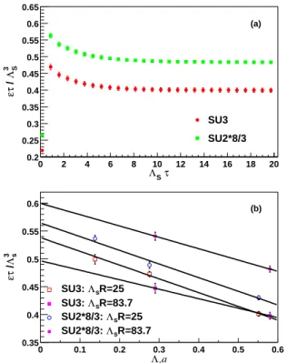
Figure 1. (a)ετ /Λ3

sas a function ofτΛsforΛsR = 83.7. (b)

ετ /Λ3

sas a function ofΛsaforΛsR= 83.7(squares) and

25(cir-cles), where a is the lattice spacing. Lines are fits of the form

a−bx.

S

Λ /

T

k

0 0.2 0.4 0.6 0.8 1

)

n(k

SU3

SU2

fit

R=83.7

Λ

(a)

0 2 4 6 8 10 12 14 16 18 20

)

n(k

10-2 SU3: ΛSR=25

R=25 S Λ SU2: R=83.7 S Λ SU3: fit

(b)

Figure 2. Transverse momentum distribution of gluons, normal-ized to the color degrees of freedom,n(kT) = ˜fn/(N

2

c−1)(see

Eq. (2)) as a function ofΛSRfor SU(3) (squares) and SU(2)

(dia-monds). Solid lines correspond to the fit in Eq.(3).

For the transverse energy of gluons, we obtain the rela-tion

1

πR2 dET

dη |η=0=

1

g2fE(ΛsR)Λ 3

s, (1)

The function fE is determined non-perturbatively as

fol-lows. In Fig. 1(a), we plot the Hamiltonian density, for a particular fixed value ofΛsR = 83.7 (on a 512×512

lattice) in dimensionless units as a function of the proper time in dimensionless units. We note that in the SU(3) case, as in SU(2),ετ converges very rapidly to a constant value. The form ofετ is well parametrized by the functional form ετ = α+βexp(−γτ). HeredET/dη/πR2 = αhas the

proper interpretation of being the energy density of pro-duced gluons, whileτD = 1/γ/Λsis the “formation time”

of the produced glue.

In Figure 1(b), the convergence of α to the contin-uum limit is shown as a function of the lattice spacing in dimensionless units for two values ofΛsR. In Ref. [21],

this convergence to the continuum limit was studied exten-sively for very large lattices (up to1024×1024sites) and shown to be linear. The trend is the same for the SU(3) re-sults. Thus, despite being further from the continuum limit for SU(3) (due to the significant increase in computer time), a linear extrapolation is justified. We can therefore extract the continuum value forα. We find fE(25) = 0.537and

fE(83.7) = 0.497. The RHIC value likely lies in this range

ofΛsR. The formation timeτD= 1/γ/Λsis essentially the

same for SU(2)-forΛsR = 83.7,γ = 0.362±0.023. As

discussed in Ref. [21], it is∼0.3fm for RHIC and∼0.13

fm for LHC (takingΛs= 2GeV and4GeV respectively).

ε= 0.17

g2 Λ

4

s. This formula gives a rough estimate of the

ini-tial energy density, at a formation time ofτD = 1/¯γ/ΛsR

where we have taken the average value of the slowly varying functionγto beγ¯= 0.34.

To determine the gluon number per unit rapidity, we first compute the gluon transverse momentum distributions. The procedure followed is identical to that described in Ref. [22] -we compute the number distribution in Coulomb gauge, ∇⊥ ·A⊥ = 0. In Fig. 2(a), we plot the normalized gluon transverse momentum distributions versuskT/Λswith the

valueΛsR = 83.7, together with SU(2) result. Clearly, we

see that the normalized result for SU(3) is suppressed

rel-ative to the SU(2) result in the low momentum region. In Fig. 2(b), we plot the same quantity over a wider range in kT/Λsfor two values ofΛsR. At large transverse

momen-tum, we see that the distributions scale exactly asN2

c −1,

the number of color degrees of freedom. This is as expected since at large transverse momentum, the modes are nearly those of non–interacting harmonic oscillators. At smaller momenta, the suppression is due to non-linearities, whose effects, we have confirmed, are greater for larger values of the effective couplingΛsR.

The SU(3) gluon momentum distribution can be fitted by the following function,

⌋ 1

πR2 dN dηd2_k

T

= 1

g2f˜n(kT/Λs), (2)

wheref˜n(kT/Λs)is

˜

fn=

(

a1hexp³p

k2

T +m2/Teff

´

−1i−1 (kT/Λs≤3)

a2Λ4

slog(4πkT/Λs)kT−4 (kT/Λs>3)

(3)

⌈

with a1 = 0.0295, m = 0.067Λs, Teff = 0.93Λs, and

a2 = 0.0343. At low momenta, the functional form is approximately that of a Bose-Einstein distribution in two dimensions even though the underlying dynamics is that of classical fields. The functional form at high momen-tum is motivated by the lowest order perturbative calcula-tions [19, 18, 26].

Integrating our results over all momenta, we obtain for the gluon number per unit rapidity, the non-perturbative result, _πR12

dN

dη|η=0 =

1

g2fN(ΛsR)Λ

2

s. We find that

fN(83.7) = 0.3. The results for a wide range ofΛsRvary

on the order of10% in the case of SU(2).

For realistic nuclei, these non-perturbative relations are less simple. One can parametrize our results for the gluon number with the more general relation

dNg

dη =fN(b)

Z

d2_x

T Λ2

s(b, xT)

g2 , (4)

where Λs(b, xT) is the local saturation scale defined to

be Λ2

s(b, xT) = C ·ρ˜(b, xT)/2, where ρ˜ is the

partici-pant density at a particular position in the transverse plane, and C is the color charge squared per nucleon. When

Λs(b, xT)=constant, as for cylindrical uniform nuclei, one

recovers the form of the expressions in Refs. [22, 23]. The color charge squared in the center of the nucleus isΛ2

s0 = C·ρ˜(0,0)/2, soΛ2

s(b, xT) = Λ2s0ρ˜(b, xT)/ρ˜(0,0). One can

then re-write the previous equation as dNg

dη = fN(b)

g2

Λ2

s0

ρ0 Npart(b), (5) where ρ0 = ρ˜(0,0) = 4.321fm−2 and Npart =

R

d2_x

Tρ˜(b, xT).

In Tables I and II, we show the calculated SU(3) results for two values of the saturation scale in the center of the nucleus: Λs0 = 1.41andΛs0 = 2.32GeV respectively. In the tables,bis an impact parameter (in units of fm) and Npart is a number of participants at that impact

parame-ter. The latter is calculated using a Woods-Saxon nuclear density profile. We list in the tables our results, as a func-tion of impact parameter, forg2_N

g; the number of produced

gluons andg2_E

g; the transverse energy of produced gluons

in GeV multiplied by the value of the strong coupling con-stant squaredg2

, evaluated (to one loop order) at the average value of the saturation scale (denoted in the tables asQs(b))

for that impact parameter.

Table I.Λs0 = 1.41GeV. In the calculation, lattice size of256×256and nuclear radius of 64 in lattice units is used. All dimensionful scales are in GeV units unless otherwise stated.

b(f m) Npart g2Ng g2Eg Λ(b) Qs(b) fN(b)

Table II.Λs0 = 2.32GeV. In the calculation, lattice size of512×512and nuclear radius of 128 in lattice units is used. All dimensionful scales are in GeV units unless otherwise stated.

b(f m) Npart g2Ng g2Eg Λ(b) Qs(b) fN(b)

0.000 377.89 3768.00 9198.736 1.9517 2.0355 0.2867 3.150 321.35 3061.59 7492.084 1.9132 1.9866 0.2757 6.300 199.11 1808.89 4183.888 1.7800 1.8185 0.2610 7.875 136.47 1215.17 2636.300 1.6560 1.6636 0.2522 8.367 118.17 1042.54 2243.692 1.6060 1.6017 0.2514 9.450 81.21 699.95 1411.900 1.4708 1.4356 0.2411

IV

Elliptic Flow

The azimuthal anisotropy in the transverse momentum dis-tribution has been proposed as a sensitive probe of the hot

and dense matter produced in ultra-relativistic heavy ion col-lisions [27]. A measure of the azimuthal anisotropy is the second Fourier coefficient of the azimuthal distribution, the elliptic flow parameterv2. Its definition [28] is

⌋

v2=hcos(2φ)i=

*

p2

x−p2y

p2

x+p2y

+

=

Rπ

−πdφcos(2φ)

R

pTdpT d

3

N dypTdpTdφ

Rπ −πdφ

R

pTdpT d

3

N dypTdpTdφ

. (6)

⌈

The first measurements of elliptic flow from RHIC, at center of mass energy √sN N, have been reported

re-cently [29]. Hydrodynamic model calculations provide good agreement, for large centralities, and for particular ini-tial conditions and equations of state, with the measured centrality dependence of the data. The agreement at smaller centralities is less good, perhaps reflecting the breakdown of a hydrodynamic description in smaller systems. Hydrody-namic models are also in excellent agreement with thept

de-pendence of the unintegrated elliptic flow parameterv2(pt)

up to 1.5 GeV/c at mid-rapidity [30]. However, above1.5

GeV, the experimental distribution appears to saturate, while the hydrodynamic model distribution continues to rise. It has been argued recently that jet quenching might explain this saturated behavour ofv2(pt)[31]. We should also note

here that hadronic transport model calculations underesti-mate the RHICv2data[29, 32].

We will now apply the classical Yang–Mills approach to compute the elliptic flow generated in a nuclear collision. As previously, we assume boost invariance–the lattice Hamilto-nian is the Kogut-Susskind HamiltoHamilto-nian in 2+1-dimensions coupled to an adjoint scalar field in Aτ _{= 0 gauge [20].}

In our earlier work, periodic boundary conditions were im-posed to compute the space–time evolution of the gauge fields after the collision [21, 22, 23]. Since, as discussed previously, elliptic flow is a consequence of an initial spa-tial anisotropy, periodic boundary conditions are inadequate and open boundary conditions are required. This technical improvement has been implemented in the work described here.

The rest of the numerical procedure is as discussed in our previous work [20, 21, 22, 23]. For each configuration

of color charges sampled forΛ2

s, we solve Hamilton’s

equa-tions on the lattice for the gauge fields and their conjugate canonical momenta. We compute the space-time evolution of the components of the Stress–Energy tensor, in particular, the two transverse components of the pressureTxx_andTyy

as well as the energy densityT00 .

In order to calculate v2 within our model, we apply the cooling method which was proposed in our previous work [22]. There we obtained, for the total number of classi-cally produced gluons, the equationN =q8

π

R∞

0

dt

√

tV(t)

whereV(t)is the potential energy for a system of free har-monic oscillators as a function of thecoolingtimet. It is clear that the gluon number defined in this manner is gauge invariant. Forv2, one can similarly prove that

v2=

R∞

0

dt

√

t(T

xx_(t)−Tyy_(t))

R∞

0

dt

√

tV(t)

. (7)

As in the case of the gluon number, this expression is gauge invariant.

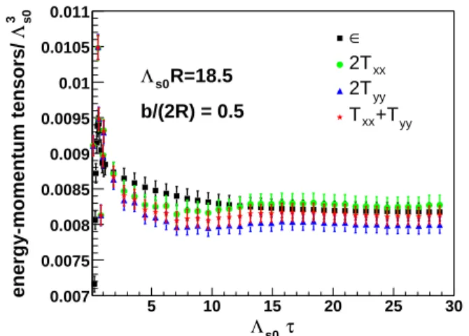
We now turn to our results [25]. In Fig. 3, we plotτ Txx,

τ Tyy and the proper timeτtimes the energy densityτ ε, in

dimensionless units as a function ofτ, also in dimensionless units, for a particular value ofΛs0Rand impact parameter

b. We observe that τ Txx andτ Tyy increase very rapidly

τ Txxandτ Tyydiffer from each other (and fromτ ε). Also,

interestingly, the energy density εat late times equals the sum of the two componentsTxxandTyy of the pressure in

the transverse plane. All of the described behavior is generic for all values ofΛs0R.

Our interpretation of the results presented in Fig. 3 is as follows. The componentsTxx andTyy of the pressure

are spatial gradients of the gauge fields. Even at the earliest times, the gauge fields decrease sharply to the edges of the “almond” characterizing the initial spatial anisotropy. One therefore gets a finite contribution toTxxandTyy. Since the

initial decrease in the gauge fields at the edges is similar in thexandydirections, the values ofTxxandTyy should be

similar in magnitude; indeed, Fig. 3 demonstrates that this is the case. Subsequently, the strong non–linear interactions of the gauge fields smooth out their spatial dependence. Even-tually, the interactions die off and the system free streams in the transverse plane. This is confirmed by the fact that ε∼Txx+Tyyat late times.

τ

s0

Λ

5 10 15 20 25 30

3 s0

Λ

energy-momentum tensors/ _0.007

0.0075 0.008 0.0085 0.009 0.0095 0.01 0.0105 0.011

∈ xx 2T

yy 2T

yy +T xx T R=18.5

s0

Λ

b/(2R) = 0.5

Figure 3. Time evolutions of energy-momentum tensor forΛsR= 18.5with the impact parameterb/2R= 0.6Lattice size128×128 andR= 32are used in the calculation.

max

/n

n

0

0.1 0.2 0.3 0.4 0.5 0.6 0.7 0.8 0.9

(%)

v

0

1

2

3

4

5

6

7

8

CG v.s.Cooling

corrected values

Figure 4. Centrality dependence ofv2 using cooling (open sym-bols) and CG (filled symsym-bols). Results are for Λs0R = 18.5 (squares), 37 (triangles), and 74 (stars). Full circles denote pre-liminarySTAR data. The band denotes estimated value ofv2at very late times. “Corrected values” is the late time cooling and CG result forΛs0R= 18.5at one centrality value.

We now turn to our result for the impact parameter de-pendence ofv2. In Fig. 4, we plotv2(computed using the definition in Eq. (7)) versusnch/nmax.

We note, as anticipated, thatv2increases with increasing impact parameter. The ratio nch/nmax is computed

self-consistently within the model. For very peripheral colli-sions, we expect that the predictions of the model are unre-liable since a hard sphere nuclear matter distribution should be replaced by a Wood-Saxon distribution in this regime. The absolute prediction of the model with the data gives about half of the observed v2. The rest of the anisotropy must be generated at later times- presumably by hydrody-namic flow. Interestingly, the dependence ofv2onΛs0Ris

rather weak. For a fixed impact parameter, a prediction of the model is that asΛs0R→ ∞, we would have the

classi-cal contribution to the elliptic flow go to zero:v2→0. This is because increasingΛsRis equivalent to increasingRand

therefore reducing the initial anisotropy. This again contra-dicts the trend in the RHIC data suggesting that the late time dynamics is important for the elliptic flow. The momentum distributionv2(pt)has also been computed in Ref. [25]. The

shape and the magnitude of this distribution also disagrees with the RHIC data.

V

The CGC and RHIC data

The classical formalism discussed here is applicable only in the initial instants of a nuclear collision. It is inapplicable once the occupation number f << 1. Moreover, the fi-nal states observed are hadrons while the CGC predicts only the initial distribution of gluons. Subsequent interactions may lead to a thermalized Quark Gluon Plasma. The pos-sibility that the CGC thermalizes has been discussed exten-sively [33]. It was argued recently that for asymptotic values of the saturation scale (Λs→ ∞) the CGC matter does

in-deed thermalize [34]. For realistic values of the saturation scale, the situation is unclear.

We will assume here, minimally, that gluonic matter formed from the CGC interacts very strongly in the trans-verse plane at early times and then free streams. Since the typical momentum of the gluons (∼ Λs) is large than the

hadronization scale (∼ΛQCD), the gluons may further

frag-ment independently before hadronizing. Invoking parton-hadron duality at parton-hadronization then enables us to compare our results to the data.

From the numerical simulations described previously we find that if we fit the total hadron multiplicity at√sN N = 130 GeV (directly equating initial num. of gluons=final num. of hadrons) we find that we obtain a value ofEt/N

that’s proportional toΛsand significantly larger than the

ob-served value (see Tables 1 & 2). Within the framework of the model, it is clear why this is the case–the CGC overesti-mates the contributions from highpt>Λs-this is more

pro-nounced inEtsince it is a more ultraviolet sensitive

global ratio ofEt/N. One still expect thatEt/Nto be

sig-nificantly larger than the measured number. NowEt/N is

not a conserved quantity and will reduce due to both inde-pendent fragmentation of the gluon “mini-jets” or hydrody-namic flow or both. Which of these is correct will become clearer once more RHIC data is available.

Kharzeev and Nardi [35] have shown that saturation+parton-hadron duality reproduces the central-ity dependence of the RHIC data. Further, Kharzeev and Levin [36] have shown that the rapidity and energy depen-dence of the RHIC data (going from √sN N = 130GeV

to√sNN = 200GeV) is predicted accurately in the same

scenario. Schaffner-Bielich et al. [37] have shown that the RHICptdata in a large kinematic region show anmtscaling

consistent with saturation. (The saturation scale extracted from themtscaling of theptspectra at different centralities

reproduces the centrality dependence of the RHIC data.) The flaw in the ointment is thev2data discussed here which disagrees with the RHIC data-this suggests the importance of final state processes and the possible thermalization of produced matter.

On a theoretical level, several improvements can be made to the picture presented here. Firstly, it would be interesting to study the effect of rapidity dependence on the gauge fields -is the system stable under rapidity depen-dent perturbations? Another interesting, if much more dif-ficult, problem is to match the classical field simulations to a kinetic approach when the occupation numbers fall below unity. This would be the appropriate time at which parton cascade type simulations would be relevant [38]. Finally, how does one extend the renormalization group treatment of the single nucleus problem to that of two nuclei. Despite the formidable challenges, we believe that the QCD based clas-sical formalism presented here is a concrete step towards a theory of high energy heavy ion collisions.

References

[1] Proceedings of International Symposium on “Statistical Me-chanics of Quarks and Hadrons”, H. Satz (ed.), Bielefeld, Aug. 24th-31st, 1980, North-Holland Publishers.

[2] J. D. Bjorken, Lectures at Int. Summer Instt. in Theoreti-cal Physics, Current Induced Reactions, Hamburg, Germany, Sept. 15th-26th, 1975, SLAC-PUB 1756.

[3] R. Anishetty, P. Koehler and L. McLerran, Phys. Rev. D22, 2793 (1980).

[4] J. D. Bjorken, Phys. Rev. D27, 140 (1983).

[5] H. Ehtamo, J. Lindfors, and L. McLerran, Z. Phys. C18, 341 (1983).

[6] J. D. Bjorken, J. Kogut, and D. Soper, Phys. Rev. D3, 1382 (1971).

[7] E. A. Kuraev, L. N. Lipatov, V. S. Fadin, Sov. Phys. JETP45

104 (1977); I. Balitsky and L. N. Lipatov, Sov. J. Nucl. Phys.

28822 (1978).

[8] F. Low, Phys. Rev. D12, 163 (1975); S. Nussinov, Phys. Rev.

14, 246, (1976).

[9] A. Donnachie and P. V. Landshoff, Phys. Lett. B296, 227 (1992).

[10] V. S. Fadin and L. N. Lipatov, Phys. Lett. B429, 127 (1998); M. Ciafaloni and G. Camici, Phys. Lett. B430, 349, (1998).

[11] L.V. Gribov, E. M. Levin and M. G. Ryskin, Phys. Repts.

100 (1983) 1; A. H. Mueller and J.-W. Qiu, Nucl. Phys. B268(1986) 427; J. P. Blaizot and A. H. Mueller, Nucl. Phys. B289(1987) 847.

[12] K. J. Eskola, K. Kajantie, P. V. Ruuskanen, and K. Tuominen, Nucl. Phys. B570, 379 (2000).

[13] L. McLerran and R. Venugopalan, Phys. Rev. D49 2233 (1994); D493352 (1994); D502225 (1994).

[14] J. Jalilian–Marian, A. Kovner, L. McLerran and H. Weigert, Phys. Rev. D555414 (1997); Y. V. Kovchegov, Phys. Rev. D

54, 5463 (1996).

[15] J. Jalilian-Marian, A. Kovner, A. Leonidov, and H. Weigert, Nucl. Phys. B504415 (1997); J. Jalilian-Marian, A. Kovner, and H. Weigert, Phys. Rev. D59014015 (1999); L. McLerran and R. Venugopalan, Phys. Rev. D59094002 (1999); E. Iancu, A. Leonidov and L. McLerran, Nucl. Phys. A692, 583 (2001); Phys. Lett. B510, 133 (2001); Phys. Lett. B510, 145 (2001).

[16] R. V. Gavai and R. Venugopalan, Phys. Rev. D54, 5795 (1996).

[17] E. Iancu, A. Leonidov and L. McLerran, arXiv:hep-ph/0202270.

[18] A. Kovner, L. McLerran and H. Weigert, Phys. Rev, D52, 3809 (1995); D52, 6231 (1995).

[19] M. Gyulassy and L. McLerran, Phys. Rev. C56, 2219 (1997).

[20] A. Krasnitz and R. Venugopalan, ph/9706329, hep-ph/9808332; Nucl. Phys. B557, 237 (1999).

[21] A. Krasnitz and R. Venugopalan, Phys. Rev. Lett.84, 4309 (2000).

[22] A. Krasnitz and R. Venugopalan, Phys. Rev. Lett.86, 1717 (2001).

[23] A. Krasnitz, Y. Nara, and R. Venugopalan, Phys. Rev. Lett.

87, 192302 (2001).

[24] A. Krasnitz, Y. Nara and R. Venugopalan, arXiv:hep-ph/0209269.

[25] A. Krasnitz, Y. Nara and R. Venugopalan, arXiv:hep-ph/0204361.

[26] Y. V. Kovchegov and D. H. Rischke, Phys. Rev. C56, 1084 (1997); S. G. Matinyan, B. M¨uller and D. H. Rischke, Phys. Rev. C56, 2191 (1997); Phys. Rev. C57, 1927 (1998); Xiao-feng Guo, Phys. Rev. D59, 094017 (1999).

[27] J.-Y. Ollitraut, Phys. Rev.46, 229 (1992); Phys. Rev. D48, 1131 (1993).

[28] S. Voloshin and Y. Zhang, Z. Phys. C70, 665 (1996); A.M. Poskanzer and S. Voloshin, Phys. Rev. C58, 1671 (1998).

[29] STAR Collaboration, K.H. Ackermann et al., Phys. Rev. Lett.

86, 402 (2001). The experimental data have been obtained from http://www.star.bnl.gov/STAR/.

[31] X. Wang and M. Gyulassy, Phys. Rev. Lett.68, 1480 (1992); M. Gyulassy, P. Levai and I. Vitev, Phys. Rev. Lett.85, 5535, (2000); U. A. Wiedemann, Nucl. Phys. A690, 731 (2001); R. Baier, D. Schiff and B. G. Zakharov, Ann. Rev. Nucl. Part. Sci.50, 37 (2000).

[32] M. Bleicher and H. St¨ocker, hep-ph/0006147.

[33] A. H. Mueller, Nucl. Phys. B572, 227 (2000); A. H. Mueller, Phys. Lett. B475, 220 (2000); J. Bjoraker and R. Venugopalan, Phys. Rev. C63, 024609 (2001); A. Dumitru and M. Gyulassy, Phys. Lett. B494, 215 (2000).

[34] R. Baier, A. H. Mueller, D. Schiff and D. T. Son, Phys. Lett.

B502, 51 (2001).

[35] D. Kharzeev and M. Nardi, Phys. Lett. B507, 121+ (2001).

[36] D. Kharzeev and E. Levin, nucl-th/0108006.

[37] L. McLerran and J. Schaffner-Bielich, Phys. Lett. B514, 29 (2001); J. Schaffner-Bielich, D. Kharzeev, L. McLerran, and R. Venugopalan, nucl-th/0108048.