Exact Solution for the Self-Organized Critical Rainfall Model
R. F. S. Andrade
Instituto de F´ısica, Universidade Federal da Bahia
Campus da Federac¸˜ao, 40210-340, Salvador, Bahia, Brazil
Received on 1 April, 2003
This work presents an analytical investigation for a Self-Organized Criticality abelian model that describes basic properties of rainfall phenomena. The knowledge of the exact solution for the probability that a site topples when mass is added to any other site of the lattice leads to a large number properties of the model, including the exponent of the power law that describes presence of the events as function of their magnitude. It is shown that the model belongs to the same universality class of a first model proposed by Dhar and Ramaswamy (DR). However, for finite size lattices, it is found that its exponent is larger than that one for the DR model.
I
Introduction
Abelian sand pile models (ASM) [1] became quite important for the understanding of basic properties of Self-Organized Criticality (SOC) [2, 3]. They satisfy the remarkable prop-erty that the final state of the model, after subsequent addi-tion of grains to any two sites, is independent of the order in which the grains have been added.
The first analyses by Dhar and Ramaswamy [4] con-sidered a model (DR) based on a critical height criterion for toppling, i.e., a site becomes unstable and topples when its amount of mass exceeds a threshold value mth. In this
model, a site topples to exactlyddistinct neighbors. This is adirectedanddeterministicmodel as, i) the toppling rules breaks the isotropy of the lattice and avalanches develop along one direction; and ii) a deterministic rule indicates the fixed number of grains that each site receives when an unsta-ble site topples. These two properties impose the condition that each site topples only once during an avalanche.
Abelian models constitute a special set where analyti-cal investigation has lead to exact results, what are still rare subjects in the SOC landscape. More recently, a number of works have focused on certain variants of abelian mod-els: they include the random distribution of toppling grains onto a restricted number of neighboring sites [6-8], and the complete toppling of all grains from an unstable site [9-11]. The first modification does keep the models in the abelian class, and an exact solution for the probability distribution function of events (PDF) has been discussed. The properties of such models are distinct from those with deterministic toppling rules. On the other hand, the second modification breaks the commutativity of the models, that seem to be non-integrable.
Other SOC models, that were initially proposed based on the so-called gradient condition for toppling, as the Bak-Tang-Wiesenfeld (BTW) model [2], also belong to this
class, provided the variables are conveniently re-interpreted. But, as far as they allow for multiple toppling for a single avalanche, they are not exactly integrable.
The exact solution for the DR model is based on the evaluation of the probability distribution functionP(s1;s0).
It measures the probability that a sites1topples when one
grain is added in a sites0,and takes into account all
config-urations of the lattice which satisfies this requirement. The knowledge ofP(s1;s0) opens the door to a large number
of properties of the model, including the functionρ(f),that measures the relative number of avalanchesρof a given size as function of the avalanche sizef.
The ASM class includes a much larger number of mod-els, some of which can be exactly integrable. A model sug-gested by a very crude description of drop avalanche inside a 2-dimensional cloud, the abelian rainfall model [5], is quite close to the original DR model. However, it allows for the presence of holes inside an avalanche cluster, what is found in the DR models only for dimensiond≥3.Although the numerical simulations suggest that this model belongs to the same universality class as thed= 2DR model, its analytical solution is still missing. Such solution can clear out whether the presence of holes inside an avalanche cluster changes or not the critical behavior of the model. The purpose of this work is to discuss a full analytical solution forP(s1;s0)of
this model, and to prove that, in the infinite lattice limit,ρ(f) is indeed described by the same exponent as in the case of the DR model. We also analyze in which extent, results for finite sizelattices for the two models differ from each other. The rest of the work is so organized: in the Section II we present the model, writing the equations forP in terms of two sub-lattices; the corresponding solutions are obtained in the Section III. Section IV discusses the relation between P andρ,and this function is evaluated with the help of the three sites probability functionP3.Section V brings results
the infinite lattice limit. Section VI closes the work with concluding remarks.
II
The two sub-lattices model
formu-lation
The model for rainfall is defined on aN ×M square lat-tice, whose axes are oriented along horizontal and vertical (downward) directions [5]. Periodic boundary conditions are imposed on the horizontal direction. Each site si on
the lattice, labeled by the indicesi = (j, k),is intended to describe a condensation nucleus, around which vapor con-denses, leading to cloud droplets with liquid water content measured by the variablemi.When a water ”grain” is
ran-domly added to a sitei, representing the growth of droplet by mass aggregation due vapor condensation, it topples if
the value formi ≥mth. This describes the downward
mo-tion when the gravitamo-tion surmounts the drag force. It is followed by collision, coalescence and drop break-up. The mass of siteiand its neighbors in the lower row are updated according to the rule:
m(j,k)→m(j,k)−mth,
m(j−1,k+1)→m(j−1,k+1)+w×mth,
m(j,k+1)→m(j,k+1)+u×mth,
m(j+1,k+1)→m(j+1,k+1)+e×mth,
(2.1)
wherew+u+e= 1.
Let us consider a site si and its corresponding
P(si;s0) =P(j, k;s0).Then, as the sitesireceives grains
from its neighbors in the upward direction, we can relate P(si;s0)with the same functions evaluated at these sites,
i.e.,
⌋
P(j, k;s0) =
1 mth
[eP(j−1, k−1;s0) +uP(j, k−1;s0) +wP(j+ 1, k−1;s0)]. (2.2)
Now we split the original lattice into two square sub-lattices,AandB, as indicated in Fig. 1. The axes of both sub-lattices are obtained from the old ones by a rotation ofπ/4followed by an inversion of the newX axis. In this reference frame, the sites are re-labeled according to:
(j, k)→hk−2j,k+2ji
A≡
h e j,eki
A, ifj+k is even,
(j, k)→hk−j+1 2 ,
k+j−1 2
i
B≡
h ej,eki
B,ifj+k is odd.
(2.3)
We observe that the row indexkis expressed in terms of the new labels byej+ek.
The equation (2.3) is rewritten in terms of two probability functionsPAandPB, which are the restrictions ofP to each of
the two sub-lattices:
PA(j, k;s0) = m1th [ePA(j, k−1;s0) +wPA(j−1, k;s0) +uPB(j, k−1;s0)],ifsi∈A
PB(j, k;s0) = m1th [ePB(j, k−1;s0) +wPB(j−1, k;s0) +uPA(j−1, k;s0)],ifsi∈B (2.4)
⌈
Figure 1. Lattice model with the two sub-lattices site labeling. The fraction of grains toppling to each site is indicated for one site of each sub-lattice. The sub-lattices are decoupled ifu= 0.
For the sake of simpler notation, we have let h
e
j,eki→[j, k] andj+k=tin (2.4) and in all expressions from now on.
If we setu= 0in (2.4), the equations for the sub-lattices decouple and become equal to that one used to describe the DR model in two dimensions. This confirms that the two models are very close, but the solutions of the equation for generalumay lead to other type of behavior.
III
Solution of the equation for
P
A particular solution to (2.4) can be evaluated after a series of steps. So let us define
PA,B(j, k;s0) =mthpA,B(j, k;s0) (3.1)
and
In terms of these new functions, the equation (2.4) becomes
⌋
¡
4j2+ 8jk+ 4k2−2j−2k¢A
j,k=eAj,k−1+wAj−1,k+uBj,k−1 ,
¡
4j2+ 8jk+ 4k2−2j−2k¢B
j,k=eBj,k−1+wBj−1,k+uAj−1,k. (3.3)
Bearing in mind the typical solutions for the DR model, we look for solutions in which the functionsZj,kbecome
separa-ble, i.e.,
Zj,k=JZ(j)×KZ(k), (3.4)
and use the following ansatz
JA(j) = A
(2j−β)!; JB(j) = B
(2j−ζ)!; KA(k) = A
(2k−η)!; KB(k) = B
(2k−ξ)!. (3.5)
⌈
Inserting (3.4) and (3.5) into (3.3), and imposing that the coefficients of the different powers ofjandkmust be equal on the different sides of the resulting expressions, we obtain several relations betweenA, B, β, ζ, η, ξand the parameters e, w andu.The evaluation of the complete set of roots to this equation is a difficult task, as the unknowns are present
in several factorials. However, the following particular so-lution, valid whene=w=u/2 = 1/mth,has been found
by inspection:
A=B = 1/2; β =η= 0; ζ=−ξ= 1. (3.6) It leads to the explicit form
⌋
PA(j, k;s0) = 1
4t+1
(2t)!
(2j)!(2k)!, PB(j, k;s0) = 1 4t+1
(2t)!
(2j−1)!(2k+ 1)! (3.7) As expected, this solution satisfies
X
j,k;j+k=t≥t0
PA(j, k;s0) +
X
j,k;j+k=t≥t0
PB(j, k;s0) = 1
4 = 1 mth
, (3.8)
wheret0=j0+k0.
⌈
The probabilitiesP(s1;s0)andP(s2;s0),fors1 6=s2,
are not independent, as there are many configurations that lead to toppling from boths1ands2.In the sum ofP(s;s0)
over all sites withtconstant, the configurations that lead toq toppling sites appear exactlyqtimes. The sums in (3.8) are equivalent to summing over individual configurations mul-tiplied by the number of toppling sites. Thus, to the average number of sites that topple when one grain is added at s0.
As mth = 4, this indicates that the average of one grain
falls from any row to each added grain, and reflects the mass conservation property of the model.
It is worth pointing out that a general analytical solution, for any values fore, uandw,may not exist in terms of the ansatz (3.5), the form of which is too restrictive. However, solutions for other values of these parameters, though not expressed in a closed compact form, can indeed be found [12]. The present solution must capture the essential global properties of this model, as different choices for the parame-ters do not change its symmetry properties. This can also be seen in the results of many different numerical simulations.
IV
The distribution of events
ρ
(
f
)
As the functionP reflects the constant flux property, it does not directly measure the sizef of avalanches, that is de-fined by the number of sites that topple. To obtain the func-tion ρ(f) we first relate f to the number of rows that an avalanche reaches. To this purpose, we have to evaluate N(t;t0),the average number of events in which the rowt
is active, i.e., in which at least one site in the rowttopples when a grain is added at rowt0. It is easy to observe that
N(t;t0) = N(t−t0; 0), so that we simplify the notation
toN(t),assuming that the grain is added att0 = 0.Thus,
the probabilityp(t)that one avalanche exceeds the rowtis N(t)/C(t),whereC(t)counts the number of distinct con-figurations of the lattice until rowt,i.e.,C(t) =mSth(t),with S(t) = (t+ 1)2indicating the total number of sites that can
m(t)that topples fromtmust increase withtα, in order to
keep the constant average flux. Then we obtain for the inte-grated massf(t)∼tα+1,so that after inverting this relation tot ∼ f1+1α , we can expresspb(f)≡p(t(f))∼ f−1+αα .
Aspb(f)expresses the probability that an avalanche exceeds the total number of sitesf,it is related toρ(f)by
ρ(f) = dpb df ∼f
−1+21+αα ≡f−τ
(4.1) The behavior of the function ρ(f) depends essentially on the behavior ofN(t).It can be expressed by
N(t) =
2Xt+1
ℓ=1
nt(ℓ) (4.2)
wherent(ℓ)counts the number of configurations in whichℓ
sites topple in the rowt. The behavior ofnt(ℓ)depends on
the values of the same function fort−1,so that a general equation can be written as
nt(ℓ) =
X
ℓ′
ct−1(ℓ, ℓ′)nt−1(ℓ−ℓ′) (4.3)
Due to the presence of holes in the avalanche clusters, the form of the coefficientsct(ℓ, ℓ′)for the rainfall model
be-comes very cumbersome as the value oftincreases. How-ever, for the DR model in two dimensions(u= 0in (2.4) andmth= 2), ct(ℓ, ℓ′)has the very simple form:
ct(ℓ, ℓ−1) =ct(ℓ, ℓ)/2 =ct(ℓ, ℓ+ 1) = 2t,
ct(ℓ, ℓ′) = 0, ℓ′6=ℓ−1, ℓ, ℓ+ 1 (4.4)
Such simple form forct(ℓ, ℓ′)is related to the fact that the
avalanches for the DR model in two dimensions have no holes. Equation (4.3) with the coefficients given by (4.4) can be numerically integrated, so that the behavior forp(t) and the value forαis easily obtained.
A possible way to side-step the difficult to evaluate (4.3) for the present model, is to consider the square average flux over the constant rowt. It is obtained by summing, over all lattice configurations until that row, the square of the number of sites that topple from the rowtfor each particular config-uration. It can also be regarded as the average flux taken with the help of other distribution that favors those config-urations with larger number of toppling. In comparison to the constant flux (eq. (3.8)), this quantity over-weights the configurations with larger number of toppling sites, so that it increases witht.Its dependence ontfollows the same rule as form(t), so that it leads to the exponentα.
To evaluate the square flux over a given rowt, we will consider the three point probability functionP3(s1, s2;s0),
where boths1ands2belong to the that row. Of course, we
must haveP(s1;s0) =P3(s1, s1;s0).This function
essen-tially counts the number distinct of configurations until that row, where boths1ands2topple. Following the same
ar-guments to identify (3.8) with the average flux, it is possible to see that, in the sumPs1,s2P3(s1, s2;s0),a given
config-uration withqtoppling sites appear exactlyq2times. As a
consequence, this sum equals the square average flux, and should increase withtα.
The equation for P3(s1, s2;s0), that looks much the
same as (2.4), now depends on two indicesZ andZ′.For
instance, takingZ=Z′ =A,we obtain:
⌋
m2
th×P3,AA(j1, k1, j2, k2) =
e2P
3,AA(j1, k1−1, j2, k2−1) +ewP3,AA(j1, k1−1, j2−1, k2)+
+euP3,AB(j1, k1−1, j2, k2−1) +weP3,AA(j1−1, k1, j2, k2−1)+
+w2P
3,AA(j1−1, k1, j2−1, k2) +wuP3,AB(j1−1, k1, j2, k2−1)+
+ueP3,BA(j1, k1−1, j2, k2−1) +uwP3,BA(j1, k1−1, j2−1, k2)+
+u2P3,BB(j1, k1−1, j2, k2−1),
(4.5)
where we dropped the explicit indication of the sites0for a simpler notation. The equations corresponding to the three other
possible choices ofZ, Z′
are very similar to (4.5).
The solution to the equations forP3can be obtained from the following ansatz:
P3,ZZ′(s1, s2;s0) = X
y
F(y−s0)PZ(s1;y)PZ′(s2;y), (4.6)
wherey−s0must be read as the difference between two vectors, and the sum overyspans all sites on the rowst′such that
t0≤t′ ≤t. Inserting (4.6) into (4.5) and the three other equivalent equations, and demanding thatP(s1;s0) =P3(s1, s1;s0),
leads to a set of equations that allows, recurrently, for the evaluation ofF(y)at all different sites. For the current purpose, however, it is sufficient to evaluate
X′
s1,s2;t
P3,ZZ′(s1, s2;s0) =
X′
s1,s2;t X
y
F(y−s0)PZ(s1;y)PZ′(s2;y), (4.7)
where the prime indicates that the sums are restricted to the sitess1ands2over a given rowt.Then we observe that
X
y
=
tX+t0
t′=t0 X′
so that (4.7) becomes: X′
s1,s2;t
P3,ZZ′(s1, s2;s0) =
tX+t0
t′=t0 X′
y;t′F(y−s0) X′
s1,s2;t
PZ(s1;y)PZ′(s2;y). (4.9)
Noting that the functionPZ(s1;y)depends only on the relative position ofs1andy,we can re-label all positions in the above
equation, settingt0= 0,so that (4.9) becomes
X′
s1,s2;t
P3,ZZ′(s1, s2;s0) =
t
X
t′=0 X′
y;t′F(y) X′
s1;t−t′
PZ(s1; 0)
X′
s2;t−t′
PZ′(s2; 0). (4.10)
DefiningFb(t) =Py′;tF(y),and using (3.8) we obtain X′
s1,s2;t
P3,ZZ′(s1, s2;s0) =
1 m2
th t
X
t′=0
b
F(t). (4.11)
To evaluateFb(t)let us consider a restricted version of (4.7), where the sums are taken fors1 =s2.In this case, (4.10)
becomes
X′
s1,s1;t
P3,ZZ(s1, s1;s0) =
t
X
t′=0
X′
y;t′F(y) X′
s1;t−t′
PZ(s1; 0)PZ(s1; 0) = 1
mth
. (4.12)
We define
Q(t) =X′
s1;t
PZ(s1; 0)PZ(s1; 0) =
1 m2
th
2t
X
ℓ=0
· (2t)!
(ℓ)!(2t−ℓ)! ¸2
(4.13)
so that (4.12) reduces to
t
X
t′=0
b
F(t)Q(t−t′) = 1
mth
(4.14)
This is a very compact way of writing the equations forF(t).It allows for a formal solutionF(t) =F(t−1)−F(0)δ(t) that can be easily computed, with
δ(t) = "
Q(t)−
t−1
X
ℓ=1
Q(ℓ)δ(t−ℓ) #
1
Q(0) (4.15)
⌈
V
Results
The square flux has been evaluated for several values of twith the help of (4.11), as shown in a logarithm plot in the Fig. 2. For the purpose of comparison, we also draw, in this figure, results for the DR model: the square flux, that has been evaluated by a similar procedure as described above, and the functionm(t),that has been evaluated with the help of eqs. (4.2-4.4). The curves for the DR model are paral-lel in the limit of large values oft,what confirms that both the square flux andm(t)depends asymptotically ontwith the same exponentα.However, it is possible to note that the curve for the rainfall model is somewhat steeper.
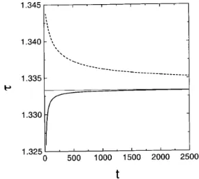
For a more accurate analysis we show, in the Fig. 3, local values for the exponentτ(t)obtained from the square flux data for both DR and rainfall models. The evaluation of the correspondingα(t)proceeds via a least square evaluation on a local window aroundt.The curves were drawn for a win-dow encompassing 10 points, but the results depends only
very weakly on the window width. We see that the exponent for the DR model converges to the asymptotic value4/3 ob-tained by Dhar from the lower side, according to power law
|4/3−t|−1. On the other hand, the exponent for the rainfall model is always greater than4/3 and decays to this value with a lower exponent∼ −0.47.
As the crucial difference between the two models lye in the presence of holes inside an avalanche cluster, the results show that they cause the rainfall model to have a smaller probability of larger events in comparison to the DR model, specially for small lattices. In the thermodynamic limit, however, the two models belong to the same universality class.
A confirmation of the above result can be obtained by exploring the properties of the analytical solution for the square flux. We see from (4.13) that the contributions to Q(t)exhibit a sharp maximum atℓ=t.Thus, we estimate
Q(t)∼ 1
m2+2th t ·
(2t)! t!t!
¸2
where∆(t)indicates the width of the peak aroundℓ = t. Making use of the Stirling approximation, we can easily show that∆(t) ∼ t1/2,while the square of the bracketed term≃(16πt)−1.Thus we obtain thatQ(t)∼t−1/2.
Figure 2. Double logarithmic plot of the square flux for both rain-fall (dotted) and DR (full) models, and of the quantitym(t)for the DR model (dashed) as function oft.The curves for the DR model are parallel, but the slope of the square flux for the rainfall model is somewhat steeper.
Figure 3. Behavior of the exponentτ for finite size lattices. The rainfall and DR models share the same exponent only in thet→ ∞
limit. For finite size lattices the probability of larger events is smaller for the rainfall model.
An asymptotic behavior forF(t)follows if we approx-imate the sum in (4.14) by an integral. Assuming that F(t)∼t−α,we must impose that the integral
t
Z
0
(t′)−α(t−t′)−1/2dt′
(5.2)
does not depend ont.As this is verified when α = 1/2, inserting this value into (4.11) leads finally to α = 1/2, the asymptotic value obtained from the numerical evalua-tion and also found for the DR model [4].
VI
Conclusions
In this work we presented an analytical investigation of an abelian SOC model that describes some aspects of rainfall. This model shares many properties of the abelian DR model, but as it allows for the presence of holes within an avalanche cluster, it has some properties of its own.
We were able to obtain an analytical solution for the probabilityP(s1;s0)that a sites1topples when one grain
is added in any other site s0 of the lattice. Knowing this
probability function is essential for the derivation of many other properties of the model. So we could evaluate the ex-ponentτ that describes the dependence of the statistics of events as function of event magnitude. Although the value ofτ coincides with that of the DR model in the limit of an infinite lattice, we have shown that for finite size lattice this exponent becomes larger than that for the DR model.
The particular solution for the rainfall model described in this work also opens the probability to analyze the be-havior of the presence of holes inside an avalanche cluster. This analysis is currently on the way and will be published elsewhere.
Acknowledgements
The author is much indebted to Dr. S.T.R. Pinho and to Prof. D. Dhar for many stimulating discussions and sugges-tions. This work has been partially supported by CNPq.
References
[1] D. Dhar, Phys. Rev. Lett.64, 1613 (1990).
[2] P Bak, C. Tang, K. Wiesenfeld, Phys. Rev. Lett 59, 381 (1987).
[3] P. Bak,How nature works: The Science of Self-Organized Criticality, (Copernicus, New York, 1996).
[4] D. Dhar and R. Ramaswamy, Phys. Rev. Lett. 63, 1659 (1989).
[5] S. T. R. Pinho and R. F. S. Andrade, Physica A 255, 483 (1998).
[6] A. Vazquez, e-print cond-mat/0003420 (2000).
[7] M. Kloster, S. Maslov, C. Tang, Phys. Rev. E 63, 26111 (2001).
[8] R. Pastor-Satorras and A. Vespignani, J. Phys. A 33, L3, (2000).
[9] M. Paczuski, K. Bassler, Phys. Rev. E62, 5347 (2000) [10] D. Hughes, M. Paczuski, Phys. Rev. Lett. 88, 054302-1
(2002)
[11] S. T. R. Pinho, R. F. S. Andrade, A. P. M. Tanajura, and S. C. Fraga, Physica A314, 405 (2002).