A Novel Iterative CT Reconstruction Approach Based on FBP Algorithm.

(1)

RESEARCH ARTICLE

A Novel Iterative CT Reconstruction

Approach Based on FBP Algorithm

Hongli Shi, Shuqian Luo, Zhi Yang, Geming Wu*

School of Biomedical Engineering, Capital Medical University of China, Beijing, China, 100069

*shl@ccmu.edu.cn

Abstract

The Filtered Back-Projection (FBP) algorithm and its modified versions are the most impor-tant techniques for CT (Computerized tomography) reconstruction, however, it may produce aliasing degradation in the reconstructed images due to projection discretization. The gen-eral iterative reconstruction (IR) algorithms suffer from their heavy calculation burden and other drawbacks. In this paper, an iterative FBP approach is proposed to reduce the aliasing degradation. In the approach, the image reconstructed by FBP algorithm is treated as the intermediate image and projected along the original projection directions to produce the reprojection data. The difference between the original and reprojection data is filtered by a special digital filter, and then is reconstructed by FBP to produce a correction term. The cor-rection term is added to the intermediate image to update it. This procedure can be per-formed iteratively to improve the reconstruction performance gradually until certain stopping criterion is satisfied. Some simulations and tests on real data show the proposed approach is better than FBP algorithm or some IR algorithms in term of some general image criteria. The calculation burden is several times that of FBP, which is much less than that of general IR algorithms and acceptable in the most situations. Therefore, the proposed algorithm has the potential applications in practical CT systems.

Introduction

Today the medical images provide very important health information in clinical diagnosis, in which X-ray CT image is one of most important modalities. The quality of CT images heavily depends upon the reconstruction algorithms, especially in the case that only less and less pro-jection data is available in order to reduce the radiation dose. The current algorithms can be roughly divided into two categories: 1) analytical reconstruction algorithms, 2) iterative recon-struction (IR) algorithms. Some of IR algorithms, such as the algorithms based on dictionary learning or compressed sensing(CS) theory, have become the research focuses and have been used in a few special fields, which can solve some reconstruction problems where projection data is far from the requirement of Shannon theorem [1–6]. However, these algorithms suffer from heavy calculation burden, poor convergence speed and other drawbacks. For example, the iteration number may be several hundreds of thousands [5], and the average computational a11111

OPEN ACCESS

Citation:Shi H, Luo S, Yang Z, Wu G (2015) A Novel Iterative CT Reconstruction Approach Based on FBP Algorithm. PLoS ONE 10(9): e0138498. doi:10.1371/ journal.pone.0138498

Editor:Huafeng Liu, Zhejiang Univ, CHINA Received:February 2, 2015

Accepted:August 31, 2015 Published:September 29, 2015

Copyright:© 2015 Shi et al. This is an open access article distributed under the terms of theCreative Commons Attribution License, which permits unrestricted use, distribution, and reproduction in any medium, provided the original author and source are credited.

Data Availability Statement:All relevant data are within the paper.

(2)

time of one iteration may be several seconds [7]. Generally, IR algorithms are based on some hypothetical conditions which are not always satisfied in practice. For example, the algorithm using total variation minimization may cause the details to be weakened or removed. On other hand, the analytical schemes, i.e. FBP algorithm and its modified versions such as FDK (Feld-kamp-Davis-Kress) algorithm, are much simpler and faster [8–14]. They have been used in almost all the fields of straight ray tomography, such as X-ray CT and PET (Positron Emission Tomography) [15–17].

For the continuous systems, Radon and inverse Radon transforms using FBP algorithm are in a close form in the mathematics principle [10,11,13]. However, it necessarily produces non-negligible aliasing degradation when the projection data and FBP algorithm have to be discretized. Many approaches had been proposed to deal with this problem. As the description in [18], a multilevel back-projection method had been presented to improve the computational speed while a point-spread-function (PSF) convolution techniques had been proposed to reduce blurring in reconstruction. As a result, the image quality was similar with or superior to that using the classic FBP technique. In [19], the spline interpolation and ramp filtering had been combined to improve the classic FBP algorithm, by which the image quality could also be improved somewhat. In [20], a new filter has been designed to substitute the classic ramp filter to improve reconstruction performance.

In this paper, an iterative CT reconstruction approach based on FBP algorithm is proposed, which is designed to hold both advantages while reduce both disadvantages of analytical and IR algorithms. In the algorithm, the classic FBP is utilized to obtain the initial reconstructed image, which is treated as theintermediateimage. It is then projected along the original projec-tion direcprojec-tions to produce thereprojectionvectors. The difference between the real and repro-jection vector is filtered by a special digital filter to produce the corrected prorepro-jection term, which is then performed the inverse Radon transform with same parameters to produce a cor-rection term in image domain. By adding the corcor-rection term to the previous one, the new intermediate image is obtained. The digital filter is designed to make the new reprojection vec-tors approach to the real projection vecvec-tors as much as possible. This procedure can be per-formed iteratively until certain stoping criterion is achieved.

Generally, the projection vectors (together with projection angles) are all the information that we have obtained about the image to be reconstructed. If the reprojection data obtained using the proposed approach better resembles the real projection data than the one obtained using the classic FBP, it is reasonable to regard the proposed approach is better than the latter one.

The digital filter is very important for the proposed approach. In order to make the idea behind the design scheme for the filter clear, the reason that produces aliasing degradation by the discretizing process is analyzed at first. Then, a correction scheme is proposed.

Methods

At first of this section, FBP algorithm is introduced in brief, and then the aliasing degradation caused by the discretizing process in FBP algorithm is analyzed. At last, an iterative scheme is proposed to reduce the aliasing degradation.

1. FBP algorithm

There are two projection modes for the general tomography: parallel beam and fan beam pro-jection. Since a reconstruction problem for the latter can be easily transformed as a problem for the former, only the former is studied in this paper.

(3)

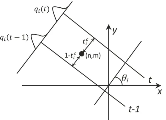
The derivation of FBP algorithm for parallel beam tomography is rather simple and straightforward [10,11]. The projection procedure can be instantiated inFig 1. The Fourier slice theorem shows that the two-dimensional (2-D) Fourier transform (FT) at frequency sam-ple (ωcosθ,ωsinθ),F(ωcosθ,ωsinθ), can be obtained by the one-dimensional (1-D) FT of projection vector at angleθ(at same time, the expression of beam lines in Cartesian coordi-nates is transformed as the expression in polar coordicoordi-nates). Therefore, the 1-D inverse FT (IFT) can substitute 2-D IFT, by which the original image can be reconstructed, namely, the inverse Radon transform is achieved. The Jacobian matrix of Cartesian-polar transformation becomes as the ramp filter.

In the calculation, the projection data and reconstructed images have to be discretized. For a discrete projection vector,pθi(t),t2[−L/2, ,L/2] (denoted bypi(t) in the next), the discrete FT (DFT) and inverse DFT (IDFT) are employed to approximate FT and IFT, respectively. The FBP algorithm becomes [8]

SiðkÞ ¼ XL

=2

t¼ L=2

piðtÞexp i2p kt N

; k2 ½ N=2_þ1_;_;_N₌2_;

qiðtÞ ¼

1

N X

N=2

k¼ N=2þ1

SiðkÞ k N exp i

2_ptk

N

;

^

fðn;mÞ ¼ p

K XK

i¼1

qiðtÞ ¼ p K

XK

i¼1

qiðbncosyiþmsinyieÞ;

ð1Þ

where^fðn;mÞdenotes the reconstructed image;Lis a positive even integer denotes the size of projection vectors;Nis an even integer that is equal to or larger than the maximum size of the projection vectors at all directions;jk

Njis the“ramp”ﬁlter in the frequency domain;bxe

Fig 1. Parallel Projection: an objectf(x,y) and its projectionpθ(t) from angleθ.

doi:10.1371/journal.pone.0138498.g001

(4)

denotes the nearest integer ofx;θi,i2[1, ,K], denote the discretized scanning angle, andK is the number of the scanning angles. Generally, FFT (fast Fourier transform) is utilized to speed up reconstruction.

2. The aliasing degradation analysis

In this subsection, the implementation of FBP is analyzed in detail to show the cause of aliasing degradation. As shown inEq (1), the implementation of FBP algorithm can be split into two steps: filtering and interpolating. The filtering can also be expressed in spatial domain as fol-lowing after IDFT and some simplifications.

qiðtÞ ¼

1

N XN

=2

k¼ N=2þ1

XL

=2

l¼ L=2

piðlÞexp i2p kl N " # k N exp i

2_ptk

N ¼ 1 N XL =2

l¼ L=2

piðlÞ XN

=2

k¼ N=2þ1

exp i2_pkl kt

N k N " # ¼ 1

4piðtÞ þ

X

t6¼l

piðtÞbNðt lÞ

ð2Þ

where

b_Nðt lÞ ¼ 1

N XN =2 k¼0 k N exp

i2_pk_ð_t _l_Þ

N

X

1

k¼ N=2þ1

k

N exp

i2_pk_ð_t _l_Þ

N

!

It is obvious thatβN(t−l) become a constant whenNisﬁxed. For example, whenN= 64,

β54(±1)−0.1014,β64(±2)0,β64(±3)−0.0113; whenN= 512,β512(±1)−0.1013, β₅₁₂(±2)0,β₅₁₂(±3)−0.0112. In fact [9],

lim

N!1bNðtÞ ¼

2

Z 1=2

0

xcosð2_tpx_Þ_dx_¼

1₌4 _t_¼0_;

0 _t_¼2_;4_;6_;_;

1

t2

p2 t¼ 1;3;5; :

8 > > > > < > > > > :

Letβ(t) denote limN! 1βN(t). WhenNis large enough such asN128,βN(t) will be

substituted byβ(t) from now on, where the error caused by substitution will be very small and can be ignored. Sinceβ(t) is symmetrical, theEq (2)can also be expressed as the circular convo-lution of the original projection vectors and a kernelhn

qiðtÞ piðtÞ hnðtÞ ð3Þ

wheredenotes the circular convolution operator,hn= [β(2n+1), ,β(3),0,β(1),

1

4;bð1Þ;0;bð3Þ;0; ;bð2nþ1Þ.

(5)

Now, suppose the reconstructed image is performed Radon transform along the identical angles again. The reprojection vector alongθiwith a distancetfrom the rotation center,p^iðtÞ, can be expressed as

^

piðtÞ ¼ X

ðn;mÞ2S

sðtÞ^fðn;mÞ

whereSdenotes the set of pixels that lies betweenxcosθi+ysinθi=t−1 andxcosθi+ysin

θi=t+ 1;s(t) indicates the weight of a pixel contributes to the projection line^piðtÞ. Since each pixel’s contribution is proportionally split into the two projection lines that sandwich the pixel according to the distances between the projection lines and the pixel,s(t) is a linear function of t. By substituting^fðn;mÞwithEq (1), the reprojection vector can be expressed as following after some simpliﬁcations

^

piðtÞ ¼ X

ðn;mÞ2S XK

j¼1

a_iðtÞqiðtÞ ð4Þ

whereα_{i(t) denotes the new coefﬁcient, which is also the linear function of}t. ConsiderEq (3), theEq (4)can further be expressed as following for briefness.

^

piðtÞ X

ðn;mÞ2S XK

j¼1

a_iðtÞpiðtÞ hnðtÞ ¼YiðtÞ hnðtÞ ð5Þ

whereY

iðtÞ ¼ P

ðn;mÞ2S PK

j¼1aiðtÞpiðtÞ.

Fig 2. Reconstruction from the filtered projection: the linear interpolation procedure.

(6)

Remark: TheEq (5)is a summary conclusion about the original projection and reprojection vectors. It can also be comprehended in the following way. Sinceqi(t)pi(t)hn(t), the inter-polation in the reconstruction and the follow-up reprojection are all linear process when the linear interpolation mode is chosen in the reconstruction process, the reprojection vector can be expressed as the circular convolution of the ramp filterhnand a term that is the linear com-bination of original projection vectors.

3. The correction scheme

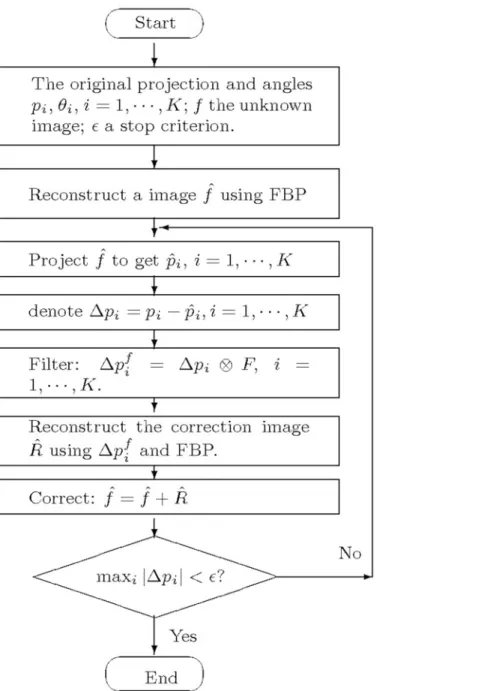
The original projection vectors (and the corresponding projection angles) are the best knowl-edge we have got about the unknown object. TheEq (5)shows there is a distinct difference between an original projection vector and the corresponding reprojection one, which indicates the imperfection degree of reconstruction. We seek to take the advantage of the original projec-tion data again in an iteraprojec-tion way to minimize the difference, in other words, improve the reconstructed image quality step by step. The proposed iterative scheme is shown as the flow-chart inFig 3.

The idea behind the processing flow is to make the reprojection vectors gradually approach the original projection vectors. First, obtain the initial reconstructed image^f by FBP algorithm.

^

f is then performed Radon transform using the identical setting to obtain the reprojection vec-tors^_p

i. Second, calculate the difference betweenpiand^pi,Dpi¼pi ^pi, which isﬁltered to produce aﬁltered projection residualΔf_pi₌Δ_pi_{F. At last, an image correction term is}

obtained byΔf_p

i, which is add to^f to update^f. The wholeﬂow can be performed iteratively. The design of the filterFbecomes a very key issue. The filter should be designed to meet the following requirement

Y_ð_t_Þ_h

nðtÞ þ ð½pðtÞ YðtÞ hnðtÞ FðtÞÞ hnðtÞ pðtÞ ð6Þ

wherep(t) denotes an original projection vector;Θ_(t)_{hn(t) denotes the corresponding}

repro-jection vector;p(t)−Θ(t)hn(t) denotes the projection residual, (p(t)−Θ(t)hn(t))F(t) denotes theﬁltered version; ((p(t)−Θ(t)hn(t))F(t))hndenotes the correction term, which is added toΘ_(t)_{hn(t) to make the updated reprojection vector approach the original}

projection vectorp(t). It requires

hnðtÞ FðtÞ ¼dðtÞ ð7Þ

whereδdenotes the discrete Dirac delta function.

In the design, supposeF(t) is symmetrical and its length is identical with that ofhn. For example,h5= [β(−5),0,β(−3),0,β(−1),1/4,β(1),0,β(3),0,β(5)],F= [x1,x2,x3,x4,x5,x6,x5,x4,

x3,x2,x1,].δ(t) is

dðtÞ ¼

(1_; _t_¼0

0_; _t_6¼0_:

orδ= [0, 0, 0, 0, 0, 1, 0, 0, 0, 0, 0]

Now the design becomes rather simple.Fwill be the solution of the question

min

F khnF dk

2

2 ð8Þ

For example, whenN= 128, i.e.,h5= [−0.0041,0,−0.0113,0,−0.1013,0.25,−0.1013, 0,

(7)

Results

In this section, some numerical simulations and tests on real data are shown to demonstrate the performance of the proposed reconstruction algorithm together with the designed filter. All animal experiments and procedures carried out on the animals are approved by the animal welfare committee of Capital Medical University and the approval ID is SCXK-(Army) 2013-X-99.

Example 1. This example is employed to show the filter designed can make the reprojection vectors approach the original projection vectors very well. The original imageIselected is the

Fig 3. The flowchart of the iterative FBP algorithm.

(8)

head phantom generated by Matlab functionphantomwith 128 × 128 pixels. It is performed Radon transform usingradonwith the angle vectorθ= [0°,1°, , 179°] to producep0. The reconstructed image^_I_{is obtained by}_iradon_{(where the classic FBP is utilized) using the linear}

interpolation mode.^_I_{is performed Radon transform again to get the reprojection vectors}_p1_.

Then, calculateΔ_pf_{= (p}0_−p1₎_{F, the correction image}_R^_{and the corrected image}^_I_þ_{R. Itera-}^

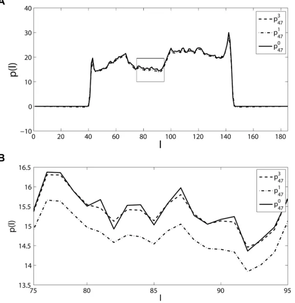
tively, a same Radon transform is performed to using the corrected image to produce new pro-jection vectors, and so on. This procedure is iterated twice following theﬂowchart inFig 3(it is only a part of the proposed algorithm as the decision process is absent). Since they are matrixes (2d), only one vector of eachp0,p1andp3(the reprojection after twice iteration) is shown in

Fig 4, whose angle isθ= 47°.

The results show that the difference between the corrected reprojection vectorp3 47andp

0 47is

much smaller than that of the reprojection vectorp1 47andp

0

47. In order to assess the efﬁciency

of the designedﬁlter, MSE (mean square error) is employed as the criterion. Let

s1¼ 1

LK XK

i¼1 kp1

i p

0

i k

2 2; s2 ¼

1

LK XK

i¼1 kp3

i p

0

i k

2

2 ð9Þ

wherep0

i,p

1

i andp

3

i denote the original, reprojection and corrected projection vectors for the projection angleθi;Lis the size of a vector, andKdenotes the number of projection angles. The results for two examples are shown inTable 1.

The results illustrate the proposed scheme together with the designed filter make the cor-rected reprojection vectors approach the true projection vectors very well.

Example 2. The original imageIis also the phantom image of 128 × 128 pixels. The angle vector is selectedθ= [0°,0.3°, , 179.7°], along whichIis projected to produce the original projectionP. It is reconstructed by the classic FBP and the proposed iterative FBP. The original image and its reconstructed versions by different schemes are shown inFig 5.

As [20], three criteria,MSE(Mean Square Error),UQI(Universal Quality Index) andMI (mutual information), are employed to assess the efficiency of the proposed approach, which are defined as following [21,22].

MSEðIr_;_Io_{Þ ¼} 1 M

ffiffiffiffiffiffiffiffiffiffiffiffiffiffiffiffiffiffiffiffiffiffiffiffiffi XM

1

k¼0 ðIr

k I o kÞ 2 s ;

whereIr kandI

0

kdenote the pixels of the reconstructed imageI r

and reference imageI°, respec-tively;Mis the total number of pixels.UQIis deﬁned as following

UQIðIr_;_Io_{Þ ¼}2CovðI r_;_Io_Þ

s2

rþs

2 0

2_Ir_Io

ð_Ir_Þ2_{þ ð}_Io_Þ2;

where_I_and_σ2_{denote the image mean and variance, respectively;}_Cov(Ir_,_{I°) denote the} covari-ance of the reconstructed imageIrand reference imageI°. The mean, variance and covariance are deﬁned as the following

_Ir _¼ 1 M

XM 1

k¼0 I

r k;

Io_¼ 1 M

XM 1

k¼0 I

o k s2 r ¼ 1 M XM 1

k¼0 ðI

r k

_Ir_Þ2

; s2

o¼

1

M XM 1

k¼0 ðI

o k

Io_Þ2

CovðIr_;_Io_Þ _¼ 1

M 1

XM 1

k¼0ðI

r k

Ir_Þð_Io k

_Io_Þ_:

(9)

Fig 4. The original projection vectorp047, the reprojection vector,p 1

47, and the corrected projection vector,p 3

47, for the head phantom of size 128 × 128

andθ= 47°.(a) The whole vector, (b) the portion of the black in (a). doi:10.1371/journal.pone.0138498.g004

Table 1. MSE of the different projection and the original projection.

Image sizeN 128 1024

Angles interval 1° 0.3°

s₁ 0.2917 11.8474

s₂ _0.0322 _0.0348

doi:10.1371/journal.pone.0138498.t001

(10)

MIis used for measuring their mutual dependence.

MIðIr_;_Io_{Þ ¼}X N0 1

k¼0

X N0 1

n¼0

pðIr k;I

o kÞlog

pðIr k;I

o kÞ pðIr

kÞpðIkoÞ

;

wherepðIr

kÞandpðI o

kÞdenote the marginal densities ofI

r_and_{I°, respectively, which are}

calcu-lated using the corresponding histograms; the joint densitypðIr k;I

o

kÞis estimated from the joint histogram ofIrandI°;N0_{denotes the number of bins in the histogram.}

UQImeasures the pixel-to-pixel similarity between the reconstructedIrand reference image I°, whileMImeasures the histogram correlation between them. The closer to 1 theUQIvalue is, the more similar the two images are. Similarly, the higher theMIvalue is, the more similar the two images are. Since it is a simulation example, the original image is known and selected as the reference image.

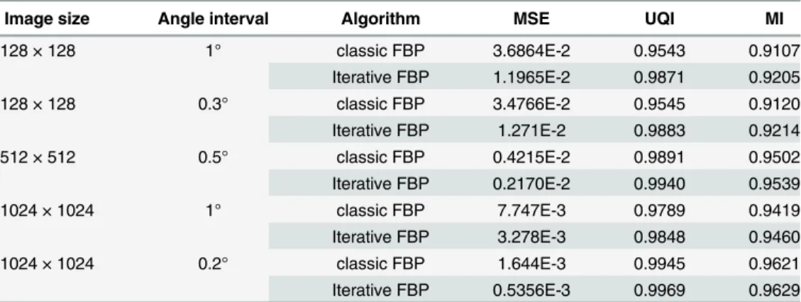
The results in the form of the three criteria are showed inTable 2, in which the phantom images with different sizes and projection settings are employed. The results illustrate the pro-posed scheme have better reconstruction performance than the classic FBP algorithm.

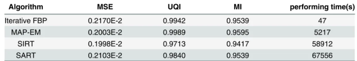
Example 3. In order to compare the iterative FBP with the current iterative schemes in the terms of speed and accuracy, some reconstruction problems are implemented by SIRT (Simul-taneous Iterative Reconstruction Technique), SART (Simul(Simul-taneous Algebraic Reconstruction Technique) and MAP-EM (Maximum A Posteriori estimation Expectation Maximization) algorithms [23–25]. Unlike the iterative schemes such as the scheme based on minimization of

Fig 5. The original image and its reconstructed versions by different schemes.(a) The original image (128 × 128), (b) the reconstructed image using the classic FBP, (c) the reconstructed image using the iterative FBP.

Table 2. The performance evaluation in Example 2.

Image size Angle interval Algorithm MSE UQI MI

128 × 128 1° classic FBP 3.6864E-2 0.9543 0.9107

Iterative FBP 1.1965E-2 0.9871 0.9205

128 × 128 0.3° classic FBP 3.4766E-2 0.9545 0.9120

Iterative FBP 1.271E-2 0.9883 0.9214

512 × 512 0.5° classic FBP 0.4215E-2 0.9891 0.9502

Iterative FBP 0.2170E-2 0.9940 0.9539

1024 × 1024 1° classic FBP 7.747E-3 0.9789 0.9419

Iterative FBP 3.278E-3 0.9848 0.9460

1024 × 1024 0.2° classic FBP 1.644E-3 0.9945 0.9621

(11)

total variation (TV) regularization or dictionary-learning, these algorithms do not make any artificial assumption on the image to be reconstructed. For the schemes based on TV minimi-zation, there is an assumption that the TV of the underlying image is minimum. For the schemes based on dictionary-learning, the assumption is that the underlying image can be expressed by a linear combination of atoms, the high-dimensional vectors, in a dictionary, the vector set. SIRT, SART and MAP-EM schemes are identical with the proposed scheme in the regard, which depend only on the projection data rather than relying on a prior information or assumption. Thus, they are chosen to compare with the proposed scheme.

The head phantom with 512 × 512 pixels is selected as the original image, which is per-formed Radon transform with the anglesθ= [0°,0.5°, , 179.5°] to produce original projection p0. The image is reconstructed using the three schemes, and the three criteria, MSE, MI and UQI are employed to evaluated the reconstruction performance. For all the schemes, the image reconstructed using the classic FBP is chosen as the initial image of iteration. The results is showed inTable 3andFig 6.

The results show that the iterative FBP algorithm has the similar reconstruction perfor-mance with SART, SIRT and MAP-EM schemes, and a much smaller operating time. We think the superiority of iterative FBP in the term of speed mainly roots in the fact that it does not employ the linear expression of projection procedure. The expression refers to a very huge matrix (see theEq (1)orEq (2)in [25] or in page 277 [8]) and will slow down the calculation, however, it is necessary for SIRT, SART and MAP-EM schemes. When the image size and the number of projection angle is large (as that in this example), the matrix becomes very huge and has to be split into many blocks. Every block has been saved and loaded at least one time, which spends many time.

In order to analyze the robustness of iterative FBP, suppose the original projection is pol-luted by the white Gaussian noise, i.e.,

p¼p0þsZ

wherep0denotes the original projection vectors, which is the Radon transform of the head

phantom image of 256 × 256 pixels with the projection anglesθ= [0°,1°, , 179°];Zis the white Gaussian noise with same size asp0, whose mean is zero and variance is one;σis the

magnitude of noise, which is selected as 0.1max(p0). The image is reconstructed using the three

schemes, SART, SIRT and MAP-EM, and Iterative FBP scheme. In all the schemes, the image that is reconstructed using the classic FBP is chosen as the initial image of iteration. The some results are showed inFig 7.

The results show that the iterative FBP algorithm has the poor but acceptable reconstruction performance, while SART, SIRT and MAP-EM have very bad performance even after a rather long running time. SIRT and MAP-EM have worse tendency than SART with the iterative recurrence proceeds. We think the weaknesses mainly roots in the fact that they depend upon

Table 3. The compare of reconstruction performance between SIRT, SART, MAP-EM and Iterative FBP (the image size is 512 × 512 and the angle interval is 0.5°).

Algorithm MSE UQI MI performing time(s)

Iterative FBP 0.2170E-2 0.9942 0.9539 47

MAP-EM 0.2003E-2 0.9989 0.9595 5217

SIRT 0.1998E-2 0.9713 0.9417 58912

SART 0.2103E-2 0.9840 0.9539 67556

doi:10.1371/journal.pone.0138498.t003

(12)

the linear expression of projection procedure, which make the reconstruction performance is very sensitive to the noise in the projection data.

Example 4. In this example, the proposed algorithm is used in the practical application. The sample is a mouse liver, and the experiment is performed in the X-ray Imaging and Biomedical Application Beamline station (BL13W1) at the SSRF(Shanghai Synchrotron Radiation Facility, China). All animal experiments and procedures carried out on the animals are approved by the

(13)

animal welfare committee of Capital Medical University and the approval ID is SCXK-(Army) 2013-X-99. The setup can ensure x-ray beam to be near parallel. The energy is about 21 keV. A CCD camera (the size of pixel is 13μm× 13μm) is used as the detector, comprising 2,588 × 458 pixels. During scanning, the sample is rotated on a turntable around its cylindrical axis by 180° at step of 0.4411°. The rotation speed is about 0.25°/sand the exposure time was 11 millisec-ond. Before and after scan, the background images (the sample is absent) and dark field images (the x-ray beam is closed) are recorded for preprocessing. The background images are used for

Fig 7. (a) The compare of MSE using SART and Iterative FBP. (b) is the portion of the first 60s of (a). doi:10.1371/journal.pone.0138498.g007

(14)

normalization, the dark field images are used to reduce the noise of various kinds(mainly cam-era noise). Finally, the logarithm transform is employed to enhance the image contrast,

pi¼ lgðpbi pidÞ lgðpoi pdiÞ

wherepb i,p

d i andp

o

i denotei-th column of background image, darkﬁeld image and projection image. The images are reconstructed by the classic FBP and the proposed iterative FBP, which are shown inFig 8.

Since there is not a reference image, it is difficult to assess the image quality by some quanti-tative indexes. The difference between the real projection vectors and the reprojection vectors, i.e.,s1ands2defined inEq (9), are employed as the criterion. In this example,s1= 299.4172,s2

= 93.4903.

Discussion

As is shown inFig 2andEq (5), the projection and reconstruction model are relatively simple in this paper. There are some factors are not considered, such as the quantization error (for example inradonfunction in Matlab, every pixel is divided into four sub-pixel and projects each sub-pixel separately) and projection noise. For such a model, the optimization ofEq (7)

orEq (8)will be rather complicated and difficult.

As previously shown in the flow chart (Fig 3), the computation burden induced by the itera-tive procedure mainly comes from the calculation of the additional reconstruction and filtering

(15)

procedures. Obviously, the reconstruction part is the dominant portion. Generally, the number of iterative loops is unnecessary to be larger than four, which means the extra calculation bur-den is only twice or triple that of the classic FBP. To the best of our knowledge, the calculation burden is much less than that of the most IR algorithms, and is acceptable in general.

In the practical applications, since there are many factors that may degrade the quality of reconstructed image, such as the eccentricity of cylindrical axis and measurement noise, the image quality cannot be improved greatly. The eccentricity of cylindrical axis is the most seri-ous factor for the iterative FBP algorithm because the distortion caused by the offset of projec-tion data will be accumulated as the iterative procedure proceeds. The larger the eccentricity of cylindrical axis is, the less times the iterative procedure should be performed. According to our experience, for the experiment setups such as in SSRF, once iterative procedure is an appropri-ate choice.

Conclusion

FBP algorithm is perfect for the continuous image model and scanning, however, the aliasing degradation cannot be avoided when the image and scanning model are discretized. Generally, there is a significant difference between the original projection data and the reprojection data using the classic FBP algorithm. Since the original projection data are the best information we have, a proper way is to take advantage of the original projection again to make the reprojec-tion data approach the original projecreprojec-tion data while improve reconstrucreprojec-tion performance.

According to the analysis, a reprojection vector can be approximately expressed as the circu-lar convolution of a certain kernel and a linear combination of the original projection vectors. The difference between the original projection and reprojection vector is served as the motiva-tion to improve the reconstrucmotiva-tion performance. It is filtered by a digital filter to compensate the difference caused by FBP, where the filter is designed to remove the filtering effect of the ramp filter. As a result, the sum of the reprojection vector and the filtered difference will approach the original projection vector. In the meantime, the filtered difference is performed inverse Radon transform and the result is added to the reconstruction image of last step to update it. This process can be repeated for several times until certain stopping criterion is satis-fied. The results of some numerical simulations and practical applications demonstrate the proposed scheme have better superiority over the classic FBP algorithm in the term of MSE, UQI and MI. The results also show the proposed scheme have much better superiority over some iterative algorithms that depend only on the projection data, such as SIRT, SART and MAP-EM, in the term of reconstruction convergence speed and robustness.

Acknowledgments

This work have been supported by National Natural Science Foundation of China (NSFC) under Grant No. 60972156 and No. 61227802, Beijing Natural Science Foundation under Grant No. 7142022, Scientific Research Common Program of Beijing Municipal Commission of Education No. KM201410025011, and Marie Curie International Research Staff Exchange Scheme (IRSES) actions under the 7th Framework Programme of the European Community under Grant No. PIRSES-GA-2009-269124.

The authors greatly appreciate all the anonymous reviewers for their comments, sugges-tions, quessugges-tions, even some revisions on language, which helped to improve the quality of this paper.

(16)

Author Contributions

Conceived and designed the experiments: HS SL. Performed the experiments: GW. Analyzed the data: ZY. Contributed reagents/materials/analysis tools: HS. Wrote the paper: HS ZY.

References

1. Thibault J B, Sauer K, Bouman C A, Heieh J. A three-dimensional statistical approach to improved image quality for multi slice helical CT. Med Phys. 2007 34: 4526–4544. doi:10.1118/1.2789499

PMID:18072519

2. Sidky E Y, Chartrand R, Pan X. Image reconstruction from few views by non-convex optimization. IEEE Nuclear Science Symposium Conference Record. 2007 3526–3530.

3. Sidky E Y, Pan X. Image reconstruction in circular cone-beam computed tomography by constrained, total-variation minimization. Phys Med Biol. 2008 53: 4777–4807. doi:10.1088/0031-9155/53/17/021

PMID:18701771

4. Masih Nilchian, Cédric Vonesch, Peter Modregger, Marco Stampanoni and Michael Unser. Fast itera-tive reconstruction of differential phase contrast X-ray tomograms. Optics Express. 2013 21(5): 5511–

5528. doi:10.1364/OE.21.005511

5. Xiao Han, Junguo Bian, Erik Ritman, Emil Sidky and Xiaochuan Pan. Optimization-based Reconstruc-tion of Sparse Images from Few-view ProjecReconstruc-tions. Phys Med Biol. 2012 57(16): 5245–5273. doi:10.

1088/0031-9155/57/16/5245

6. Jingyan Xu, Taguchi K, Tsui BMW. Statistical projection completion in X-ray CT using consistency con-ditions. IEEE Trans Med Imag. 2010 29: 1528–1540. doi:10.1109/TMI.2010.2048335

7. Qiong Xu, Hengyong Yu, Xuanqin Mou, Lei Zhang, Jiang Hsieh and Ge Wang. Low-dose X-ray CT reconstruction via dictionary learning. IEEE Trans Med Imag. 2012 31(9):1682–1697. doi:10.1109/

TMI.2012.2195669

8. Kak Avinash C, Slaney M. Principles of Computerized Tomographic Imaging. New York: IEEE Press, 1988.

9. Hsieh J. Computed Tomography-Principles, Designs, Artifacts, and Recent Advances. Bellingham WA: SPIE Press, 2003.

10. Faridani A. Introduction to the mathematics of computed tomography -Inside Out: Inverse Problems. MSRI Publications. 2003 47:1–46.

11. Natterer F. The Mathematics of Computerized Tomography. SIAM Philadelphia 2001.

12. Herman GT. Fundamentals of computerized tomography: Image reconstruction from projection, 2nd edition. Springer, 2009.

13. Riedert A, Faridanit A. The semidiscrete filtered backprojection algorithm is optimal for tomographic inversion. SIAM J Numer Anal. 2003 41:869–892. doi:10.1137/S0036142902405643

14. Ye Y, Wang Q. Filtered backprojection formula for exact image reconstruction from cone-beam data along a general scanning curve. Med Phys. 2005 32:42–48. doi:10.1118/1.1828673PMID:15719953

15. Zamyatin A A, Taguchi K, Silver M D. Practical hybrid convolution algorithm for Helical CT reconstruc-tion. IEEE Trans Nuc Sci. 2006 53:167–174. doi:10.1109/TNS.2005.862973

16. Anja Borsdorf, Rainer Raupach, Thomas Flohr and Joachim Hornegger. Wavelet based noise reduc-tion in CT-images using correlareduc-tion analysis. IEEE Trans Med Imag. 2008 27: 1685–1703. doi:10.

1109/TMI.2008.923983

17. Ivakhnenko V I. A novel quasi-linearization method for CT image reconstruction in scanners with a multi-energy detector system. IEEE Trans Nuc Sci. 2010 57:870–879. doi:10.1109/TNS.2010.

2042066

18. Brandty A, Jordan M, Brodskiy M, Galun M. A fast and accurate multilevel inversion Of the radon trans-form. SIAM J Appl Math. 1999 60(2):437–462. doi:10.1137/S003613999732425X

19. Horbelt S, Liebling M, Unser M. Filter design for filtered back-projection guided by the interpolation model. Proc. SPIE 4684, Medical Imaging 2002: Image Processing. 2002 May. Available:http:// proceedings.spiedigitallibrary.org/proceeding.aspx?articleid=1313610

20. Hongli Shi, Shuqian Luo. A novel scheme to design the filter for CT reconstruction using FBP algorithm. BioMedical Engineering OnLine 2013 12:50. doi:10.1186/1475-925X-12-50

(17)

22. Zhou Wang, Alan C. Bovik. A universal Image Quality Index. IEEE Signal Processing Letters 2002 9 (3): 81–84. doi:10.1109/97.995823

23. Baoyu Dong. Cone-beam Image Reconstruction Using an Improved MAP-EM Algorithm. Journal of Computational Information Systems 2012 8(19): 7839–7845.

24. Krol A, Bowsher E, Manglos H, Feiglin H, Tornai P, Thomas D. An EM algorithm for estimating SPECT emission and transmission parameters from emissions data only. IEEE Trans Med Imag. 2001 20 (3):218–232. doi:10.1109/42.918472

25. Van Tessa, Wuyts Sarah, Goossens Maggie, Batenburg Joost, Sijbers Jan. The implementation of iter-ative reconstruction algorithms in MATLAB. Available:http://www.researchgate.net/publication/ 265200864