Iterative nonlocal total variation regularization method for image restoration.

for Image Restoration

Huanyu Xu, Quansen Sun , Nan Luo, Guo Cao, Deshen Xia*

School of Computer Science and Technology, Nanjing University of Science and Technology, Nanjing, Jiangsu, China

Abstract

In this paper, a Bregman iteration based total variation image restoration algorithm is proposed. Based on the Bregman iteration, the algorithm splits the original total variation problem into sub-problems that are easy to solve. Moreover, non-local regularization is introduced into the proposed algorithm, and a method to choose the non-non-local filter parameter non-locally and adaptively is proposed. Experiment results show that the proposed algorithms outperform some other regularization methods.

Citation:Xu H, Sun Q, Luo N, Cao G, Xia D (2013) Iterative Nonlocal Total Variation Regularization Method for Image Restoration. PLoS ONE 8(6): e65865. doi:10.1371/journal.pone.0065865

Editor:Xi-Nian Zuo, Institute of Psychology, Chinese Academy of Sciences, China

ReceivedNovember 30, 2012;AcceptedApril 29, 2013;PublishedJune 11, 2013

Copyright:ß2013 Xu et al. This is an open-access article distributed under the terms of the Creative Commons Attribution License, which permits unrestricted use, distribution, and reproduction in any medium, provided the original author and source are credited.

Funding:This work was supported by grants from Programs of the National Natural Science Foundation of China (61273251, 61003108), (http://www.nsfc.gov. cn) Doctoral Fund of Ministry of Education of China (200802880017) (http://www.cutech.edu.cn) and the Fundamental Research Funds for the Central Universities

analysis, decision to publish, or preparation of the manuscript.

Competing Interests:The authors have declared that no competing interests exist.

* E-mail: ssun@126.com

Introduction

Image restoration is a classical inverse problem which has been extensively studied in various areas such as medical imaging, remote sensing and video or image coding. In this paper, we focus on the common image acquisition model: an ideal imageu[Rnis observed in the presence of a spatial invariance blur kennel A[Rn|nand a additive Gaussian white noise n[Rn with zero mean and standard deviations. Then, the observed imagef [Rn is obtained by:

f~Auzn: ð1Þ

Restoring the ideal image from the observed image is ill-posed since the blur kennel matrix is always singular. A common way to solve this problem is to use regularization methods, in which regularization terms can be invited to restrict the solutions. Regularization methods generally have the form as follows:

argmin

u DDAu{fDD

2_{zlR(u), ð2Þ}

where DD:DD denotes the Euclidean norm, lis a positive regulari-zation parameter balancing the fitting term and the regulariregulari-zation term, R(u) is the regularization term. The total variation regularization proposed by Rudin, Osher and Fatemi [1] (also called the ROF model) is a well known regularization method in this field. The total variation norm has a piecewise smooth regularization property, thus the total variation regularization can preserve edges and discontinuities in the image. The uncon-strained ROF model has the form

arg min

u DDAu{fDD

2_zlDDuDD

TV, ð3Þ

where the termDDuDD_TV stands for the total variation of the image. The continuous form of the total variation is defined as

DDuDD_TV~ ð

V

D+u(t)Ddt: ð4Þ

Many numerical methods was proposed to solve (3). WhenAis an identity matrix, the ROF model (3) turns into a TV denoising problem, methods as Chambolle’s projection method [2], semi-smooth Newton methods [3], multilevel optimization method [4] and split Bregman method [5]. WhenAis a blur kennel matrix, (3) turns into a TV deblurring problem, we have prime-dual optimization algorithms for TV regularization [6–9], forward backward operator splitting method [10], interior point method [11], majorization-minimization approach for image deblurring [12], Bayesian framework for TV regularization and parameter estimation [13–15], using local information and Uzawa’s algo-rithm [16,17], using regularized locally adaptive kernel regression [18], augmented Lagrangian methods [19,20] and so on. However, the problem is far from perfectly solved, problems as edge and detail preserving [21,22], ringing effect reducing [23–25] and varied blur kennels and noise types image restoration [26,27] still need better solutions.

The purpose of this paper is to propose an effective total variation minimization algorithm for image restoration. The algorithm is based on Bregman iteration which can give significant improvement over standard models [28]. Then, we solve the q

No. NUST2011ZDJH26. The funders had no role in study design, data collection and

proposed algorithm by alternately solving a deblurring problem and a denoising problem [29,30]. In addition, we propose a local adaptive nonlocal regularization approach to improve the restoration results.

The structure of the paper is as follows. In the next section, an iterative algorithm for total variation based image restoration is proposed, moreover we present a nonlocal regularization under the proposed algorithm framework with local adaptive filter parameter to improve the restoration results. Section Experiments shows the experimental results. Section Conculsions concludes this paper.

Methods

Iterative Approach for TV-based Image Restoration

Bregman iteration for image restoration. We first con-sider a general minimization problem as follows:

arg min

u lJ(u)zH(u,f), ð5Þ wherelis the regularization parameter,Jis a convex nonnegative regularization functional and the fitting functional H is convex nonnegative with respect toufor fixedf. This problem is difficult to solve numerically when J is non-differentiable, and the Bregman iteration is an efficient method to solve the minimization problem.

Bregman iteration is based on the concept of ‘‘Bregman distance’’. The Bregman distance of a convex functional J(:)

between pointsuandvis defined as:

Dp_J(u,v)~J(u){J(v){vp,u{vw, ð6Þ

where p[LJ is a sub-gradient of J at the point v. Bregman distance generally is not symmetric, so it is not a distance in the usual sense, but the Bregman distance measures the closeness of two points.Dp_J(u,v)§0for anyuandv, andDp_J(u,v)§Dp_J(w,v)for all points w on the line segment connecting u and v. Using Bregman distance (6), the original minimization problem (5) can be solved by an iterative procedure:

ukz1 _{~ arg min}

u lD pk

J (u,uk)zH(u,f)

pkz1 _{~ p}k_{LH(ukz1_,f),

8

<

:

ð7Þ

whereLH(ukz1_{,f)denotes a sub-gradient ofHatu}kz1_andlw0.

When we chooseH(u,f)~DDAu{fDD2 andJ(u)~DDuDD_TV, (7) turns into the total variation minimization problem, then (7) can be converted into the following two step Bregman iterative scheme [28]:

ukz1 _{~ arg min}

u lDDuDDTVzDDAu{f

k_DD2 _{ð Þ8}

fkz1 _{~ f}k_zf{Aukz1_{: ð Þ9}

(

In [28], the authors mentioned that the sequence uk _weakly converges to a solution of the unconstrained form of (5), and the sequenceDDAuk_{fDD2_{converges to zero monotonically. We can see}

from (8),(9) that,the Bregman iteration just turns the original problem (5) into a iteration procedure and add the noise residual

back into the degenerated image at the end of every iteration. Bregman iteration converges fast and gets better results than standard methods. Bregman iteration was widely used in varied areas of image processing [5,31–33].

General framework of the iterative algorithm. As intro-duced above, we use the Bregman iteration (8),(9) to bulid the main iterative framework. Rather than considering (3), we consider the problem as follows:

arg min

u,g DDAg{fDD

2_zlDDuDD

TVsubject to g~u: ð10Þ

We separated the variable u in (3) into two independent variables, so we can split the original problem (3) into sub-problems which are easy to solve. This problem is obviously equivalent to (3). We can replace (10) into the unconstrained form:

arg min

u,g DDAg{fDD

2_zl

1DDg{uDD2zl2DDuDDTV: ð11Þ

l1 and l2 are regularization parameters balancing the three

terms. If the regularization parameter l1 is big enough, the

problem (11) is close to the problem (10), and the solutions of the problems are similar. If we letJ(u,g)~DDAg{fDD2_zl

2DDuDDTV and

H(u,g)~DDg{uDD2, we can see thatJ andH are all convex, and then (10) is a simple application of (7). Thus, the above problem can be solved by using Bregman iteration:

(ukz1_,gkz1_{) ~ arg min}

u,g J(u,g){vpu

k_,u{uk_w

{vpgk,g{gkwzl1DDg{uDD2

pukz1 ~ puk{l1(ukz1{gkz1)

pgkz1 ~ pgk{l1(gkz1{ukz1):

8 > > > > < > > > > : ð12Þ

Similar to [28], we can reform the above procedure into a simple two step iteration algorithm:

ukz1_,gkz1

~arg min u,g Ag{f

2

zl₂ u _TVzl₁ g{u{bk 2 ð Þ13

bkz1_~bk_zukz1_{gkz1_{: ð Þ14}

(

As we can see in (13), when l1 tends to infinity, the above

algorithm is equal to the original Bregman iterative algorithm in [28]. we use an alternating minimization algorithm [29,30] to solve (13). We split (13) into a deblurring and a denoising sub-problems. Thus, (13) can be solved by the following two step iterative formation:

gkz1_{~arg min}

g kAg{f

2_zl

1 g{uk{bk

2

ð15Þ

ukz1_{~arg min}

u l1 g

kz1_{u{bk 2_zl

2kukTV: ð Þ16

8 < :

We can see that (15) is anl2_{-norm differentiable problem, we}

can solve it as follows:

gkz1_~(1

l1

AAT_zI){1₍1

l1

AT_fzuk_zbk_{), ð17Þ}

where I is the identity matrix and the matrix 1

l₁AAtzI is

invertible. Then (15) can be solved by optimization techniques such as Gauss-Seidel, conjugate gradient or Fourier transform. As for (16), it is a exact total variation denoising problem, we can use Chambolle’s projection algorithm [2], semismooth Newton method [3] or split Bregman algorithm [5] to solve this problem. Thus, the proposed alternating Bregman iterative method for image restoration can be formed as follows:

Algorithm 1: Alternating Bregman iterative method for image restoration.

Initializek~0 andb0_~u0

n~0 while _uk_n{uk{1

n

ukn

vtor kvmaxitertimesdo

fori~1:ndo

ukz1 0 ~ukn

gkz_i 1~arg min g Ag{f

2

zl1 g{ukzi{11{b

k 2

ukz_i 1~arg min u l1 g

kz1

i

{u{bk 2

zl2kukTV end

bkz1_~bk_zukz1

n {gk z1

n

k~kz1

end

Analysis of the proposed algorithm. First, we show some important monotonicity properties of the Bregman iteration proposed in [28].

Theorem 1 The sequence H(uk,f) obtained from the Bregman iteration is monotonically nonincreasing. And assume that there exists a minimizer ~uu[BV(V) of H(:,f) such that

J(~uu)v?. Then.

H(uk,f)ƒH(~uu,f)z

J(~uu)

k , ð18Þ

and, in particular,ukis a minimizing sequence.

Moreover,ukhas a weak-* convergent subsequence inBV(V), and the limit of each weak-* convergent subsequence is a solution ofAu~f. If~uuis the unique solution ofAu~f, thenuk?~uuin the weak-* topology inBV(V).

Then, we show that the alternating minimization algorithm (15) and (16) also convergence to the solution of the sub-problem (13) [30]. LetLbe the difference matrix andNULL(:)denotes the null space of the corresponding matrix, we obtain the following theorem.

Theorem 2 For any initial guess u0[Rn

2

, suppose fuig is generated by (15) and (16), thenuiconverges to a stationary point

of (10). And whenAis a matrix of full column rank,uiconverges to a minimizer of (10).

Then, we can get the following convergence theorem of the proposed alternating Bregman iterative method.

Theorem 3LetAbe a linear operator, consider the algorithm 1. Suppose fuig is a sequence generated by algorithm 1, ui converges to a solution of the original constrained problem (3).

Proof.Letfuigandfgigbe the sequence obtained from (13), and everyuiis the solution of the (13), moreoverH(u,g)~ku{gk2?0 with the increase in iterations of the algorithm 1. Suppose in one iteration, there isu _{and g satisfying u~g, and let the true} solutions of the problem (10) be~uuand~gg, then.

u{g

k k~k_~uu{_~ggk~0: ð19Þ

Due tou_{andgsatisfy (11),uandgcan enable the convex} function (11) to obtain its Minimum value. Then.

DDAg{fDD2zl1DDg{uDD2zl2DDuDDTV ƒDDA~gg{fDD2zl1DDgg~{~uuDD2zl2DD~uuDDTV:

ð20Þ

Thus, we can obtain.

DDAg{fDD2zl2DDuDDTV ƒDDAg~g{fDD2zl2DD~uuDDTV: ð21Þ

Owning to~uuand~ggare the true solutions of the problem (10), this inequality implies thatu_{andgare also the solutions of the} problem (10), thus are the solutions of the original unconstrained problem (3).

Connection with other methods. We noticed that the equation (17) can be rewrite as follows:

gkz1_~uk_zbk_{(AT_Azl

1I)AT(A(ukzbk){fk), ð22Þ

thus, the proposed algorithm 1 can be interpreted as follows:

gkz1 _{~ u}k_zbk_{(AT_Azl

1I)AT(A(ukzbk){fk)

ukz1 _{~ arg min}

u l2DDuDDTVzl1DDg{u{b k_DD2

bkz1 _{~ b}k_zukz1_{gkz1_:

8 > > < > > : ð23Þ

The preconditioned Bregmanized nonlocal regularization (PBOS) algorithm [33] can be formed as:

gkz1 _{~ u}k_{dAT_(AAT_z){1_(Auk_{fk₎

ukz1 _{~ arg min}

u mDDuDDTVz

1

dDDu{gk

z1_DD2

fkz1 _{~ f}k_zf{Aukz1_:

8 > > < > > : ð24Þ

the left and right pseudo inverse approximation are equal: Figure 1. Convergence speed between algorithm 1, operator splitting TV, FTVd and FAST-TV.A.7|7Gaussian kernel withsigma~3 and gaussian noise withs~2B.9|9average kernel and gaussian noise withs~3. The figure shows the convergence speed between four methods using the Cameraman image and two different blur kennels. Axis X stands for the iteration times, Axis Y stands for the relative difference between restored images in two iterations, that isDDuk_{uk{1_DD

uk_. doi:10.1371/journal.pone.0065865.g001

AT(AATzE){1~(ATAz){1_AT _ð25Þ Compare these two methods, we can see the only difference between them is the way to calculate the noise and add it back to the iteration. The PBOS method calculates the undeconvolutioned noise and only add it back to the calculation of g, while the proposed method calculate the deconvolutioned noise and add it back to both the calculations of g and u, we believe that is why the proposed algorithm have a faster converge speed and better restoration results according to the experiments in section 0.

Adaptive Nonlocal Regularization

Nonlocal regularization. Recently, nonlocal methods have been extensively studied, the nonlocal means filter was first proposed by Buades et al [34]. The main idea of the nonlocal means denoising model is to denoise every pixel by averaging the other pixels with similar structures (patches) to the current one. Based on the nonlocal means filter, Kindermann et al. [35] tried to investigate the use of regularization functionals with nonlocal correlation terms for general inverse problems. Inspired by the graph Laplacian and the nonlocal means filter, Gilboa and Osher defined a variational framework based nonlocal operators [36]. In Figure 2. Restoration results on a256|256Cameraman image degraded by a7|7Gaussian kernel withsigma~3and a gaussian noise withs~2. A. Original Image B. Degraded Image C. Operator Splitting TV D. ForWard E. FTVd F. FAST-TV G. NLTV+BOS H. Algorithm 1 I. Algorithm 2.

the following, we use the definitions of the nonlocal regularization functionals introduced in [36].

LetV5R2,x[V, u(x)is a real function V?Randwis a nonnegative symmetric weight function. Then the nonlocal gradient+wu(x)is defined as the vector of all partial differences +wu(x,:)atx:

+wu(x,y)~(u(y){u(x))

ffiffiffiffiffiffiffiffiffiffiffiffiffi w(x,y)

p

,

and the graph divergencedivw of a vector p:V|V?Rcan be defined as:

divwp(x)~

ð

V

(p(x,y){_p(y,x))pffiffiffiffiffiffiffiffiffiffiffiffiffi_w(x,y)dy,

the weight function is defined as the nonlocal means weight function:

w(x,y)~exp {(GaDDf(xz

:₎{f(yz:)DD2)(0) 2h2

, ð26Þ

whereGais the Gaussian kernel with standard deviationa,his the filtering parameter related to the standard variance of the noise, Figure 3. Restoration results on a256|256Cameraman image degraded by a9|9average kernel and a gaussian noise withs~2. A. Original Image B. Degraded Image C. Operator Splitting TV D. ForWard E. FTVd F. FAST-TV G. NLTV+BOS H. Algorithm 1 I. Algorithm 2.

doi:10.1371/journal.pone.0065865.g003

and the:inf(xz:)stands for a square patch centered by pointx. When the reference imagef is known, the nonlocal means filter is a linear operator. The definition of the weight function (26) shows that the value of the weight is significant only when the patch

aroundyhas similar structure as the corresponding patch around x.

The nonlocal TV norm can be defined as isotropicL1_{norm of}

the weighted graph gradient+wu(x): Table 1. PSNR and SSIM results of the methods on five

different images with a7|7Gaussian kernel withsigma~3 and gaussian noises~₂.

Image

Blur/noise

variance PSNR SSIM

Operator splitting 25.81 0.701

ForWARD 26.18 0.682

FTVd 25.71 0.818

Cameraman FAST-TV 26.20 0.813

NLTV+BOS 26.00 0.830

Algorithm 1 26.40 0.830

Algorithm 2 27.21 0.832

Operator splitting 23.52 0.667

ForWARD 23.79 0.701

FTVd 23.12 0.667

Barbara FAST-TV 23.28 0.706

NLTV+BOS 23.59 0.732

Algorithm 1 23.65 0.701

Algorithm 2 23.89 0.734

Operator splitting 25.88 0.716

ForWARD 25.61 0.654

FTVd 25.49 0.762

Man FAST-TV 25.65 0.755

NLTV+BOS 25.99 0.780

Algorithm 1 26.06 0.781

Algorithm 2 26.37 0.786

Operator splitting 27.60 0.813

ForWARD 27.30 0.799

FTVd 26.21 0.825

Boats FAST-TV 26.78 0.821

NLTV+BOS 28.01 0.843

Algorithm 1 27.45 0.841

Algorithm 2 28.05 0.844

Operator splitting 27.29 0.799

ForWARD 27.08 0.791

FTVd 26.46 0.824

Lenna FAST-TV 27.09 0.812

NLTV+BOS 27.52 0.836

Algorithm 1 27.54 0.832

Algorithm 2 28.00 0.836

Operator splitting 26.02 0.739

ForWARD 25.99 0.725

FTVd 25.40 0.779

Average FAST-TV 25.80 0.781

NLTV+BOS 26.22 0.804

Algorithm 1 26.22 0.797

Algorithm 2 26.70 0.806

doi:10.1371/journal.pone.0065865.t001

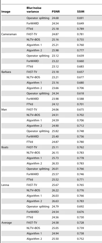
Table 2.PSNR and SSIM results of the methods on five different images with a9|9average kernel and gaussian noises~₃.

Image

Blur/noise

variance PSNR SSIM

Operator splitting 24.68 0.691

ForWARD 24.54 0.649

FTVd 25.18 0.789

Cameraman FAST-TV 24.87 0.781

NLTV+BOS 25.16 0.755

Algorithm 1 25.21 0.760

Algorithm 2 25.98 0.777

Operator splitting 23.12 0.639

ForWARD 23.22 0.660

FTVd 23.12 0.683

Barbara FAST-TV 23.18 0.657

NLTV+BOS 23.21 0.677

Algorithm 1 23.16 0.680

Algorithm 2 23.66 0.706

Operator splitting 24.34 0.618

ForWARD 23.98 0.588

FTVd 24.12 0.701

Man FAST-TV 24.06 0.675

NLTV+BOS 24.51 0.702

Algorithm 1 24.59 0.706

Algorithm 2 24.90 0.712

Operator splitting 25.82 0.748

ForWARD 25.40 0.736

FTVd 24.87 0.780

Boats FAST-TV 25.11 0.762

NLTV+BOS 26.15 0.783

Algorithm 1 25.73 0.778

Algorithm 2 26.33 0.783

Operator splitting 26.01 0.766

ForWARD 25.57 0.746

FTVd 25.52 0.771

Lenna FAST-TV 25.67 0.765

NLTV+BOS 26.22 0.776

Algorithm 1 26.03 0.766

Algorithm 2 26.63 0.783

Operator splitting 24.79 0.692

ForWARD 24.54 0.676

FTVd 24.56 0.730

Average FAST-TV 24.58 0.728

NLTV+BOS 25.05 0.739

Algorithm 1 24.94 0.738

Algorithm 2 25.50 0.752

JNLTV,w(u)~

ð

V

D+wu(x)Ddx (27)

~ ð V ffiffiffiffiffiffiffiffiffiffiffiffiffiffiffiffiffiffiffiffiffiffiffiffiffiffiffiffiffiffiffiffiffiffiffiffiffiffiffiffiffiffiffiffiffiffiffiffiffi ð V

(u(x){u(y))2w(x,y)dy s

dx: (28)

The main idea of the nonlocal regularization is to generalize the local gradient and divergence concepts to the nonlocal form. Then the nonlocal means filter is generalized to the variational framework.

The nonlocal means filter and the nonlocal regularization functionals can reduce noise efficiently and preserve textures and contrast of the image. Generally, it is good to choose a reference image as close as possible to the original ideal image to calculate the weights. However, the original image structures are broken in the degraded image, we can not get the precise weights between the pixels, thus the weights should be calculated from a preprocessed image [37]. In our alternating minimization frame-work, we get the deblurred image at the first step, then denoise the deblurred image at the second step. As the nonlocal regularization functionals are robust to the noise, and the structures of the deblurred image are close to the original ideal image, we can calculate the weights by using the deblurred image as the reference image, then apply a nonlocal denoising step to obtain the restored image.

Adaptive nonlocal parameter selection. Within the alter-nating Bregman iterative method, we can use gkz1 _{as the}

reference image to calculate the weights of the nonlocal regularization functionals, then use the weights to denoise the deblurred imagegkz1_{at every iteration. Note that the nonlocal}

filter parameterhis related to the standard variance of the noise, however we do not know the exact noise of the image gkz1_.

Moreover, when we use the single filter parameterhfor the whole image, there will be regions oversmoothed or undersmoothed in the restored image, because a single filter parameter h is not optimal for all the patches in the image. As the nonlocal TV norm defined in (27), we will calculate the filter parameterhadaptively using local information and get the localhfor every pixel in the image.

Inspired by local regularization in [21], we define the local power as:

Pr(x,y)~ 1 DVD

ð

V

(I(x0,y0){Ir(x0,y0))2Vx,y(x0,y0)dx0dy0, ð29Þ

and Vx,y(x’,y’)~V(Dx{x’D,Dy{y’D) is a normalized smoothing window, here we use a Gaussian window.Iris the expected image, Vis a region to calculate the local power centered at(x,y).

Then we use the local power to calculate the localhas follows:

h(x,y)~a ffiffiffiffiffiffiffiffiffiffiffiffiffiffiffiPr(x,y)

p

: ð30Þ

The advantage of localizing the filter parameterhis that it can control the denoising process over image regions according to their content, the smooth regions have average w between there neighbors, texture and edge regions have big wonly when the patches are similar. Besides, we do not have to know or estimate the noise condition. In this paper, we use a preprocessed oversmoothed image us as the expected image instead of the mean of the patch to get more accurate results. The oversmoothed

image is obtained by a standard TV model using a large regularization parameter.

By applying the above adaptive nonlocal regularization, the algorithm 1 can be reformed as the following algorithm, whereW is the function to calculate the weights between points andusis the preprocessed oversmoothed image:

Algorithm 2: Adaptive nonlocal alternating Bregman iterative method for image restoration.

Initializek~0 andg0 0~u0n~0 while _uk_n{uk{1

n

ukn

vtor kvmaxitertimesdo

fori~1:ndo

ukz1 0 ~ukn

gkz_n 1~arg min

g kAg{fk

2

zl1 g{ukzn{11{b

k 2

wkz1

n ~W gk z1

n ,us,a

ukz1

n ~arg min_u l1 gkzn 1{u{b k 2

zl2k ku NLTV=w end

bkz1_~bk_zukz1

n {gk z1

n

k~kz1

end

Experiments

In this section, we present some experimental results of the proposed alternating Bregman method and the adaptive nonlocal alternating Bregman method, and compare them with the operator splitting TV regularization [10], NLTV based BOS algorithm, FTVd algorithm [38], FAST-TV [30] and ForWaRD algorithm [39]. The ForWaRD algorithm is a hybrid Fourier-wavelet regularized deconvolution (ForWaRD) algorithm that performs noise regularization via scalar shrinkage in both the Fourier and wavelet domains.

We use the conjugate gradient method to solve the first subproblem in algorithm 1 and algorithm 2, use the Chambolle’s projection algorithm to solve the second subproblem in algorithm 1 and the nonlocal version of the Chambolle’s projection algorithm in algorithm 2. In algorithm 1 and algorithm 2, we set l1~0:02 and l2~0:01 by experiment results, the inner

iteration timesncan be set as1or2and the stopping condition is DDuk_{uk{1_DD=DDuk_DDv10{3_{. There are lots of work on determining}

the parameters in the regularization [40,41], but this work is out of the scope of this paper and we will get in to it later. In algorithm 2, we set the patch size as5|5, searching window as21|21and set the Gaussian variance parameter ass~5 to calculate the local variance. And we set the nonlocal parameter factor asa~2. For the operator splitting method, the regularization parameter is set as 0:1. For the NLTV based BOS method, the regularization parameter is set asl~0:2, searching window is set as21|21, the patch size is set as5|5and the nonlocal filter parameter is set as h~30. For the FTVd algorithm, we setm~1000. For the FAST-TV, we seta1as0:003and0:005according to the degeneration of

the image. And the best valve ofa1. For the ForWaRD algorithm,

we set the threshold as3sigma,sigmais the standard deviation of the noise, and the regularization parameter is set to1.

First, we compare the convergence speed of the proposed algorithm 1 with the preconditioned BOS algorithm, the FTVd algorithm and the FAST-TV algorithm in Figure 1. We can find that the proposed algorithm 1 converge faster than the other three methods at first, and still much faster than the preconditioned BOS algorithm and the FTVd algorithm later, close or a little bit slower than the FAST-TV at the end of the iterations. Usually, the stopping condition of the relative difference is set to10{3_or10{4_.

Thus, the proposed algorithm 1 can reach the stopping condition with fewer iterations than other algorithms. In terms of the computation time, the FTVd algorithm is the fastest owning to its strategies and code optimization. And the proposed algorithm 1 is faster than the operator splitting algorithm and the FAST-TV algorithm. As for the nonlocal methods, convergence can not be promised after some iterations, so we compare the computation time between these methods. As the computation of the nonlocal weights, the nonlocal based algorithms cost more computing time than the non nonlocal ones. The NLTV based BOS algorithm stops with 25 steps for 180 seconds, and the preconditioned NLTV based BOS algorithm stops with 8 steps for 75 seconds, however the proposed algorithm 2 stops with 5 steps for only 47 seconds.

Next, we show some image restoration results of these methods to illustrate the effectiveness of the proposed algorithms. We use the classical Cameraman image, so as to be comparable to other image restoration works. The Cameraman image can be found at http://www.imageprocessingplace.com/root_files_V3/

image_databases.htm. Figure 2 and Figure 3 show the restoration results on the Cameraman with two kind of blur kernels. We can see from the results that, the ForWard method can get a good restoration result when the image is not slightly blurred, but poor on the heavily blurred situation, besides the ForWard method can not restore edges clearly. The restoration results of the operator splitting TV method have artificial strips which affect the visual

appearance of the restored images. FTVd method and FAST-TV can effectively remove noise from the degenerated images, and have higher PSNRs than the ForWard method and the operator splitting TV method, however, a lot of details are also smoothed. The results of the proposed algorithm 1 have good visual appearance, clear edges and preserved image contrast. The NLTV based BOS method (the preconditioned BOS has almost the same result) and the proposed algorithm 2 have better restoration results than the not nonlocal ones, and the proposed algorithm 2 have more details restored and a higher PSNR.

The Table 1 and Table 2 shows the restoration results on 5

different images and2different degradation situations. We can see that, the PSNR and SSIM of the proposed algorithms are generally higher than the methods being compared.

Conclusions

In this paper, we propose a Bregman iteration based total variation image restoration algorithm. We split the restoration problem into a three step iteration process, and these steps are all easy to solve. In addition, we propose a nonlocal regularization under the framework of the proposed algorithm using a point-wise local filter parameter, and a method to adaptively determine the filter parameter. Experiments show that the algorithm converges fast and the adaptive nonlocal regularization method can obtain better restoration results. In the future, we will consider the weights updating problem in a theoretical way and apply the proposed algorithms for other regularization problems such as compressed sensing.

Author Contributions

Conceived and designed the experiments: HX QS. Performed the experiments: HX GC. Analyzed the data: HX QS DX. Wrote the paper: HX NL GC.

References

1. Rudin L, Osher S, Fatemi E (1992) Nonlinear total variation based noise removal algorithms. Physica D: Nonlinear Phenomena 60: 259–268. 2. Chambolle A (2004) An Algorithm for Total Variation Minimization and

Applications. Journal of Mathematical Imaging and Vision 20: 89–97. 3. Ng MK, Qi L, Yang Yf, Huang Ym (2007) On Semismooth Newton’s Methods

for Total Variation Minimization. Journal of Mathematical Imaging and Vision 27: 265–276.

4. Chan T, Chen K (2006) An optimization-based multilevel algorithm for total variation image denoising. Multiscale Model Simul 5: 615–645.

5. Goldstein T, Osher S (2009) The split Bregman method for L1 regularized problems. SIAM Journal on Imaging Sciences 2: 323–343.

6. Hintermller M, Stadler G (2006) An infeasible primal-dual algorithm for tv-based inf-convolutiontype image restoration. SIAM Journal on Scientific Computing 28: 1–23.

7. Esser E, Zhang X (2009) A general framework for a class of first order primal-dual algorithms for TV minimization. UCLA CAM Report : 1–30. 8. Carter J (2001) Dual methods for total variation-based image restoration.

University of California Los Angeles.

9. Esser J (2010) Primal Dual Algorithms for Convex Models and Applications to Image Restoration, Registration and Nonlocal Inpainting. University of California Los Angeles.

10. Combettes PL,Wajs VR (2005) Signal recovery by proximal forward-backward splitting. Multiscale Modeling Simulation 4: 1168–1200.

11. Nikolova M (2006) Analysis of half-quadratic minimization methods for signal and image recovery. SIAM Journal on Scientific computing 27: 937–966. 12. Oliveira JaP, Bioucas-Dias JM, aT Figueiredo M (2009) Adaptive total variation

image deblurring: A majorization-minimization approach. Signal Processing 89: 1683–1693.

13. Chantas G, Galatsanos N, Likas A, Saunders M (2008) Variational Bayesian image restoration based on a product of t-distributions image prior. IEEE transactions on image processing 17: 1795–805.

14. Babacan SD, Molina R, Katsaggelos AK (2008) Parameter estimation in TV image restoration using variational distribution approximation. IEEE transac-tions on image processing 17: 326–39.

15. Chantas G, Galatsanos NP, Molina R, Katsaggelos AK (2010) Variational bayesian image restoration with a product of spatially weighted total variation image priors. IEEE transactions on image processing 19: 351–62.

16. Almansa A, Ballester C, Caselles V (2008) A TV based restoration model with local constraints. Journal of Scientific Computing 34: 612–626.

17. Bertalmio M, Caselles V, Rouge´ B (2003) TV based image restoration with local constraints. Journal of Scientific Computing 19: 95–122.

18. Takeda H, Farsiu S, Milanfar P (2008) Deblurring using regularized locally adaptive kernel regression. IEEE transactions on image processing 17: 550–63. 19. Wu C, Tai XC (2010) Augmented Lagrangian method, dual methods, and split Bregman iteration for ROF, vectorial TV, and high order models. SIAM Journal on Imaging Sciences 3: 300–339.

20. Pang ZF, Yang YF (2011) A projected gradient algorithm based on the augmented Lagrangian strategy for image restoration and texture extraction. Image and Vision Computing 29: 117–126.

21. Gilboa G, Sochen N (2003) Texture preserving variational denoising using an adaptive fidelity term. Proc VLSM.

22. Li F, Shen C, Shen C, Zhang G (2009) Variational denoising of partly textured images. Journal of Visual Communication and Image Representation 20: 293– 300.

23. Prasath VS, Singh A (2009) Ringing Artifact Reduction in Blind Image Deblurring and Denoising Problems by Regularization Methods. 2009 Seventh International Conference on Advances in Pattern Recognition : 333–336. 24. Liu H, Klomp N, Heynderickx I (2010) A perceptually relevant approach to

ringing region detection. IEEE transactions on image processing 19: 1414–26. 25. Nasonov A (2010) Scale-space method of image ringing estimation. IEEE

International Conference on Image Processing (ICIP) : 2793–2796.

26. Chen DQ, Zhang H, Cheng LZ (2010) Nonlocal variational model and filter algorithm to remove multiplicative noise. Optical Engineering 49: 077002. 27. Nikolova M (2004) A variational approach to remove outliers and impulse noise.

Journal of Mathematical Imaging and Vision 20: 99–120.

29. Wang Y, Yang J, Yin W, Zhang Y (2008) A New Alternating Minimization Algorithm for Total Variation Image Reconstruction. SIAM Journal on Imaging Sciences 1: 248.

30. Huang Y, Ng MK,Wen YW (2008) A Fast Total Variation Minimization Method for Image Restoration. Multiscale Modeling & Simulation 7: 774. 31. Yin W, Osher S, Goldfarb D (2008) Bregman iterative algorithms for

l1-minimization with applications to compressed sensing. SIAM J Imaging Sci 1: 143––168.

32. Cai JF, Osher S, Shen Z (2009) Linearized Bregman Iterations for Frame-Based Image Deblurring. SIAM Journal on Imaging Sciences 2: 226–252. 33. Zhang X, Burger M, Bresson X, Osher S (2010) Bregmanized Nonlocal

Regularization for Deconvolution and Sparse Reconstruction. SIAM Journal on Imaging Sciences 3: 253–276.

34. Buades A, Coll B, Morel JM (2005) On image denoising methods. SIAM Multiscale Modeling and Simulation 4: 490–530.

35. Kindermann S, Osher S, Jones PW (2005) Deblurring and Denoising of Images by Nonlocal Functionals. Multiscale Modeling & Simulation 4: 1091–1115.

36. Gilboa G, Osher S (2008) Nonlocal operators with applications to image processing. Multiscale Model Simul 7: 1005–1028.

37. Lou Y, Zhang X, Osher S, Bertozzi A (2009) Image Recovery via Nonlocal Operators. Journal of Scientific Computing 42: 185–197.

38. Wang Y, Yin W (2007) A fast algorithm for image deblurring with total variation regularization. CAAM Technical Report TR07–10.

39. Neelamani R, Choi H, Baraniuk R (2002) Forward: Fourier-wavelet regularized deconvolution for ill-conditioned systems. IEEE Trans on Signal Processing 52: 418–433.

40. Wen Y (2009) Adaptive Parameter Selection for Total Variation Image Deconvolution. Numerical Mathematics: Theory, Methods and Applications 2: 427–438.

41. Liao H, Li F, Ng MK (2009) Selection of regularization parameter in total variation image restoration. Journal of the Optical Society of America A 26: 2311–2320.