HESSD
7, 9067–9121, 2010Data assimilation for flood forecasting
S. Ricci et al.
Title Page
Abstract Introduction
Conclusions References
Tables Figures
◭ ◮
◭ ◮
Back Close
Full Screen / Esc
Printer-friendly Version Interactive Discussion
Discussion
P
a
per
|
Dis
cussion
P
a
per
|
Discussion
P
a
per
|
Discussio
n
P
a
per
|
Hydrol. Earth Syst. Sci. Discuss., 7, 9067–9121, 2010 www.hydrol-earth-syst-sci-discuss.net/7/9067/2010/ doi:10.5194/hessd-7-9067-2010
© Author(s) 2010. CC Attribution 3.0 License.
Hydrology and Earth System Sciences Discussions
This discussion paper is/has been under review for the journal Hydrology and Earth System Sciences (HESS). Please refer to the corresponding final paper in HESS if available.
Correction of upstream flow and hydraulic
state with data assimilation in the context
of flood forecasting
S. Ricci1, A. Piacentini1, O. Thual1,2, E. Le Pape3, and G. Jonville4
1
URA CERFACS/CNRS, URA 1875, Toulouse, France
2
INPT, CNRS, IMFT, Toulouse, France
3
SCHAPI, Toulouse, France
4
CERFACS, Toulouse, France
Received: 28 September 2010 – Accepted: 5 November 2010 – Published: 30 November 2010
Correspondence to: S. Ricci ([email protected])
HESSD
7, 9067–9121, 2010Data assimilation for flood forecasting
S. Ricci et al.
Title Page
Abstract Introduction
Conclusions References
Tables Figures
◭ ◮
◭ ◮
Back Close
Full Screen / Esc
Printer-friendly Version Interactive Discussion
Discussion
P
a
per
|
Dis
cussion
P
a
per
|
Discussion
P
a
per
|
Discussio
n
P
a
per
|
Abstract
The present study describes the assimilation of river water level observations and the resulting improvement of the river flood forecast. The BLUE algorithm was built on top of the one-dimensional hydraulics model MASCARET. The assimilation algorithm folds in two steps: the first one is based on the assumption that the upstream flow can
5
be adjusted using a three-parameter correction, the second one consists in directly correcting the hydraulic state. This procedure is applied on a four-day sliding window over the whole flood event. The background error covariances for water level and discharge are represented with asymmetric correlation functions where the upstream correlation length is bigger than the downstream correlation length. This approach is
10
motivated by the implementation of a Kalman Filter algorithm on top of an advection-diffusion toy model. The assimilation study with MASCARET is carried out on the Adour and the Marne Vallage (France) catchments. The correction of the upstream flow as well as the control of the hydraulic state along the flood event leads to a significant improvement of the water level and discharge in analysis and forecast modes.
15
1 Introduction
River streamflow forecast is a challenging issue for the security of the persons and the infrastructures, the exploitation of power plants and the management of water ressources. Many efforts have been made on the development of open channel flow modeling, based on mass, momentum and energy conservation equations (Chow,
20
1959; Hervouet, 2003). Still, the uncertainties on these models are such that river streamflow modeling remains a streneous work. Major uncertainties come from the model itself as the physics are simplified and then discretized, but also from hydro-logical boundary conditions (upstream flow or lateral additional discharge), meteoro-logical boundary conditions (precipitation, pressure and wind) and from hydrometeoro-logical
25
HESSD
7, 9067–9121, 2010Data assimilation for flood forecasting
S. Ricci et al.
Title Page
Abstract Introduction
Conclusions References
Tables Figures
◭ ◮
◭ ◮
Back Close
Full Screen / Esc
Printer-friendly Version Interactive Discussion
Discussion
P
a
per
|
Dis
cussion
P
a
per
|
Discussion
P
a
per
|
Discussio
n
P
a
per
|
as numerical parameters (stability coefficient for the numerical scheme), geometry pa-rameters (cross sections, gates and weir dimensions) and hydraulic papa-rameters (flood plain storage, friction, discharge). Calibrating a hydraulics model often means adjusting Strickler coefficients, discharge coefficients at cross or lateral devices, seepage values or cross section geometry. The calibration of these parameters has been widely
inves-5
tigated (Beven and Freer, 2001; Malaterre et al., 2010) focusing either on calibration algorithms, sensitivity indications or optimality of the observations network.
Both parameter calibration and physical field description can be formulated as in-verse problems (Tarantola, 1987). The formulation of the inin-verse problem in hydrol-ogy fits into a wider mathematical framework presented by Maclaughlin and Townley
10
(1996). Data assimilation combines numerical and observational information on a sys-tem in order to provide a better description of it (Ide et al., 1997; Boutier and Courtier, 1999; Kalnay, 2003). The benefit of data assimilation has already been greatly demon-strated in meteorology (Parrish and Derber, 1992; Rabier et al., 2000) and oceanogra-phy (Brasseur and Verron, 2006) over the past decades, especially for providing initial
15
conditions for numerical forecast. Data assimilation is now being applied with increas-ing frequency to hydrology (Thirel et al., 2010, Part I; Thirel et al., 2010, Part II, ) and hydraulics problems with two main objectives: optimizing model parameters and im-proving streamflow simulation and forecast. The literature proposes several methods based on minimization techniques approaches (Atanov et al., 1999; Das et al., 2004;
20
Honnorat et al., 2007; Bessi `eres et al., 2007). The filtering approach, e.g. Kalman fil-ter or Monte Carlo algorithms, also enables the estimation of roughness coefficients (Sau et al., 2010; Pappenberger et al., 2005) and the correction of the physical fields (Jean-Baptiste et al., 2010).
The present study describes the assimilation of river water level observations and
25
HESSD
7, 9067–9121, 2010Data assimilation for flood forecasting
S. Ricci et al.
Title Page
Abstract Introduction
Conclusions References
Tables Figures
◭ ◮
◭ ◮
Back Close
Full Screen / Esc
Printer-friendly Version Interactive Discussion
Discussion
P
a
per
|
Dis
cussion
P
a
per
|
Discussion
P
a
per
|
Discussio
n
P
a
per
|
the context of data assimilation for mono-dimensional hydraulics. Asymmetric corre-lation functions are used to represent the spatial error correcorre-lations for water level and discharge. This choice is motivated by an example on a simplified model. For that purpose, a Kalman Filter algorithm is implemented on top of an advection-diffusion toy model. This exercice shows that the analysis and the dynamics of the physics modify
5
a gaussian correlation function into an asymmetric function at the observation point. The assimilation study with MASCARET is performed on the Adour (France) and the Marne Vallage (France) catchments. The improvement of the water level, using data assimilation, in analysis and forecast modes are shown. Most illustrations in this paper present the results on the Adour catchment.
10
The outline of the paper is as follows. Section 2 describes the assimilation system, paying particular attention to the choice of the control vector for the BLUE algorithm. Two approaches are implemented: the correction of the hydraulic state and the con-trol of the upstream flow. The modeling of the background covariances matrix and the parametrization for the control of the upstream flow are highlighted. Section 3 gives
15
the theoretical frame for the choice of asymmetric correlation functions for the spatial error correlations in the background error covariance matrix B. For the MASCARET application, the correlation length scale is estimated following the evolution of a per-turbation on the initial state. In Sect. 4, the improvement of the river flood simulation and forecast is presented. The evaluation of usual hydraulics criteria such as
preci-20
HESSD
7, 9067–9121, 2010Data assimilation for flood forecasting
S. Ricci et al.
Title Page
Abstract Introduction
Conclusions References
Tables Figures
◭ ◮
◭ ◮
Back Close
Full Screen / Esc
Printer-friendly Version Interactive Discussion
Discussion
P
a
per
|
Dis
cussion
P
a
per
|
Discussion
P
a
per
|
Discussio
n
P
a
per
|
2 Context and implementation of the data assimilation
2.1 Modeling of the physics
MASCARET is a one-dimensional free surface hydraulics model developed by EDF and CETMEF1, based on the Saint-Venant equations (Goutal and Maurel, 2002). MASCARET is widely used for the modeling of river flood, submersion waves resulting
5
from hydraulic infrastructure breaking, river control and canal waves propagation. The conservative form of the mono-dimensional Saint Venant equations reads:
∂S
∂t +
∂Q ∂x =qa,
∂Q
∂t +
∂ ∂x(Q
2/S
)+gS∂Z
∂x =−
gQ2
SKs2RH4/3
. (1)
In this formulation the river sectionS is expressed in m2 and is, at each locationx, a function of the water heighth=Z(x,t)−Zbottom(x,t) where Z(x,t) is the free surface
10
height in m. The discharge in m3s−1is denoted by Q(x,t), qa(x,t) is the lateral lineic discharge,Ksis the Strickler coefficient,RHis the hydraulic radius andgis the gravity.
The non stationnary mode of MASCARET is used in this study. Significant uncer-tainties on the input parameters of MASCARET, such as the Strickler coefficient or the upstream flow and lateral discharge, result in errors on the simulated water level and
15
discharge. The aim of our data assimilation approach is to reduce the uncertainties of either the inputs or the outputs of the simulation.
2.2 The assimilation method BLUE
The Best Linear Unbiased Estimator (BLUE) approach (Gelb, 1974; Talagrand, 1997) identifies the optimal estimator of the true value of an unknown variablex. This
es-20
timator is optimal as its variance is minimum, meaning, for gaussian cases, that its probability density function is dense around its mean. x is the control vector and can
1
HESSD
7, 9067–9121, 2010Data assimilation for flood forecasting
S. Ricci et al.
Title Page
Abstract Introduction
Conclusions References
Tables Figures
◭ ◮
◭ ◮
Back Close
Full Screen / Esc
Printer-friendly Version Interactive Discussion
Discussion
P
a
per
|
Dis
cussion
P
a
per
|
Discussion
P
a
per
|
Discussio
n
P
a
per
|
stand for the state variables (water level and discharge for MASCARET), the model parameters (Strickler coefficients), the boundary conditions (upstream flows) or the ini-tial condition (iniini-tial water level and discharge), or a mix of these. The solution of the BLUE algorithm is the analysis vectorxa. The a priori knowledge of the system is the background vectorxb and the observation vector isyo. The background, observation
5
and analysis error covariances are respectively gathered in the matricesB,Rand A. Assuming that the background, the observation and the analysis are unbiased, the analysis can be formulated as a correction to the background state defined as:
xa=xb+Kd, (2)
whereKis the gain matrix andd is the innovation vector
10
d=yo−H(xb), (3)
andy=H(x) is the model equivalent of the observations through the observation op-eratorH.
The BLUE analysis is optimal as the variance of its error is minimum. Minimizing the variance of the analysis comes down to minimizing the trace of the analysis error
15
covariance matrix and leads to the formulation of the gain matrix (Boutier and Courtier, 1999):
K=BHT(HBHT+R)−1. (4)
In this formulation,His the Jacobian matrix ofH around the background statexbthat can be written as:
20
H=∂y
∂x=
∂H(x)
∂x . (5)
The analysis error covariance matrix reads
A=(I−KH)B. (6)
Real-time forecast systems for meteorology and oceanography usually rely on the cycling of such algorithm, though the solution is often identified through a minimisation
25
HESSD
7, 9067–9121, 2010Data assimilation for flood forecasting
S. Ricci et al.
Title Page
Abstract Introduction
Conclusions References
Tables Figures
◭ ◮
◭ ◮
Back Close
Full Screen / Esc
Printer-friendly Version Interactive Discussion
Discussion
P
a
per
|
Dis
cussion
P
a
per
|
Discussion
P
a
per
|
Discussio
n
P
a
per
|
The analysis at time i−1 is propagated in time by the dynamical model Mi−1,i to
define the background at timei (Eq. 7). It is then corrected to provide the analysis xai
at timei given by Eq. (8).
xbi =Mi−1,i(xai−1), (7)
xa i =x
b
i +Ki
h
yo i −Hi(x
b
i)
i
, (8)
5
with
Ki=BiHTi (HiBiHTi +Ri)−1, (9)
whereMi−1,i represents the model propagation betweeni−1 and i of the physics in Eq. (1),Bi,Ri are the background and observation error covariance matrices at timei
andHi is the observation operator at timei andHi is its linear approximation at timei.
10
The analysis error covariance matrixAi−1is computed from Eq. (10) at each
assim-ilation time. The analysis error covariance matrix at timei−1 is propagated in time by the dynamical model to define the background error covariance matrix at timei as written in Eq. (11), whereMi−1,i is the tangent linear approximation ofMi−1,i.
Ai−1=(I−Ki−1Hi−1)Bi−1 (10)
15
Bi =Mi−1,i Ai−1MTi−1,i. (11)
Equations (7–10) are the Kalman Filter equations (Todling and Cohn, 1994) with no error model. If the gain matrixKi is kept constant over time andMi−1,i=Iis assumed,
then they come down to the BLUE equations applied in our study.
2.3 Implementation of the assimilation scheme
20
HESSD
7, 9067–9121, 2010Data assimilation for flood forecasting
S. Ricci et al.
Title Page
Abstract Introduction
Conclusions References
Tables Figures
◭ ◮
◭ ◮
Back Close
Full Screen / Esc
Printer-friendly Version Interactive Discussion
Discussion
P
a
per
|
Dis
cussion
P
a
per
|
Discussion
P
a
per
|
Discussio
n
P
a
per
|
MASCARET reveals the model difficulties to catch the rise in the water level and to of-ten underestimate the flood peak for moderate events and overestimate the flood peak for important flood events. Two data assimilation schemes were implemented on top of the MASCARET model.
2.3.1 Correction of the hydraulic state
5
The first data assimilation approach consists in dynamicall correcting the water level and the discharge states for the entire catchment (discretized inmcells) when obser-vations are available. In this case, the control vector is composed of the discretized water level and discharge statesx=Zx1,···,Zxm,Qx1,···,Qxm
=(Z,Q).
The background state is given by a previous integration of the model, it is the
sim-10
ulated water level and discharge state denotedZb,Qb. The size of the control and the background vectors isn=2 m. The observation vector contains water level at ob-servation times and at selected locations on the hydraulic network. It is a vector of sizepwherep is the number of observations. The observation operator sums up to a selection matrixp×n, denoted byHsel that can be written as
15
Hsel=
0···1···0···0···0 ..
. ... ... ... ... ... ... ... ... 0···0···1···0···0
..
. ... ... ... ... ... ... ... ... 0···0···0···1···0
where the non zero values correspond to the location of the observation point on the state vectorx. When the observation points do not correspond to positions on the grid, the selection matrixHsel then represents an interpolation operation or a neighbouring
operation.
HESSD
7, 9067–9121, 2010Data assimilation for flood forecasting
S. Ricci et al.
Title Page
Abstract Introduction
Conclusions References
Tables Figures
◭ ◮
◭ ◮
Back Close
Full Screen / Esc
Printer-friendly Version Interactive Discussion
Discussion
P
a
per
|
Dis
cussion
P
a
per
|
Discussion
P
a
per
|
Discussio
n
P
a
per
|
The observation covariance matrix R is a p×p matrix. Its diagonal terms are the observation error variances at the observation points and the off-diagonal terms are the covariances between the observation errors at different observation points. The background covariance matrix is an×nsymmetric positive-definite matrix that can be represented by blocks:
5
B=
BZ,Z B
T
Z,Q
BZ,QBQ,Q
.
Then×ndiagonal blocksBZ,ZandBQ,Q represent the statistics for the errorsǫZ of the
water level andǫQof the discharge, respectively. Its diagonals represent the variance
of the background error for the water level and the discharge respectively whereas the extra diagonal terms of these blocks are the covariances between the error on
10
the water level or the discharge at different locations on the grid. These covariances are commonly defined asunivariateas opposed to themultivariatecovariances in the extra-diagonal blocksBZ,Q andB
T
Z,Qthat represent the covariances between the errors
on the water level and the errors on the discharge.
The innovation vectord (Eq. 3) expresses the difference between the simulated and
15
the observed water level at observation pointsxobs and times. At these locations, since
the observation operator is a simple selection operator in our case, the innovation is weighed by the matrix productHTsel(HselBH
T
sel+R)− 1
in Eq. (4): f
δZ=HTsel(HselBHTsel+R)−1d (12)
whereδfZ is the water level correction vector at the observation points that reads
20
f
δZ=(δgZ1,···,δgZl,···,δgZp) (13)
withl∈ {1,···,p}.
Water level correction δZ for the whole domain results from the multiplication of f
δZ by BZ,Z. The water level variances translate the uncertainties on the simulated
water level. An asymmetric correlation functionρis used to describe the spatial error
HESSD
7, 9067–9121, 2010Data assimilation for flood forecasting
S. Ricci et al.
Title Page
Abstract Introduction
Conclusions References
Tables Figures
◭ ◮
◭ ◮
Back Close
Full Screen / Esc
Printer-friendly Version Interactive Discussion
Discussion
P
a
per
|
Dis
cussion
P
a
per
|
Discussion
P
a
per
|
Discussio
n
P
a
per
|
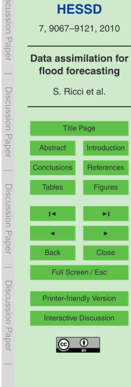
correlations onδZ. The correlation function at an observation point such thatxobs=
250 is presented on Fig. 1.
The correlations depend on the curvilinear distance between two points and the correlation length was computed with a systematic procedure of propagation of a local perturbation (see Sect. 3).
5
The discharge correction vector at the observation point δfQ=(δQg1,···,δQgl,···) with l∈ {1,···,p}, is deduced from δZf at the observation points using the proportionality relation:
g
δQl=
Qbl
ZlbδZgl, (14)
whereQbl and Zlb are the background values for the water level and discharge at the
10
obervation points. As for the water level, the discharge correction δQ for the whole domain results from the multiplication of δfQ by BQ,Q. The correlation function and length forδQare those used forδZ. Complementary work on the modeling of (δfZ,δfQ) error covariances modeling was initiated using a physical calibration procedure at each observation point such as
15
g
δQl=a(gδZl)r+b (15)
withl∈[1,p]. Still, because of the tide influence at some observation points, the iden-tification of a satisfactory approximation of these relations valid for both high tide and low tides was not always possible.
2.3.2 Correction of the upstream flow
20
HESSD
7, 9067–9121, 2010Data assimilation for flood forecasting
S. Ricci et al.
Title Page
Abstract Introduction
Conclusions References
Tables Figures
◭ ◮
◭ ◮
Back Close
Full Screen / Esc
Printer-friendly Version Interactive Discussion
Discussion
P
a
per
|
Dis
cussion
P
a
per
|
Discussion
P
a
per
|
Discussio
n
P
a
per
|
part of the error on the simulated water level can be attributed to the uncertainty on these upstream free extremities. In order to control the uncertainty on this upstream flow, a data assimilation procedure was set up. For this approach, the control vector should contain the discharge boundary conditions at the upstream stations over the simulation period. The relation between the control space and the observation space
5
is given by the integration of the numerical model, this operation being non linear. Still, the correction of the upstream flow for each model time step would involve a large control vector and a heavy assimilation procedure, especially for the computation of the Jacobian of the observation operator.
For that reason, the upstream flow forcingf is corrected through three linear
trans-10
formations over a time window (assimilation window): e
f(t)=af(t−c)+b. (16)
The characteristics of this data assimilation approach are:
– The background values for the control parameters arexb=(ab,bb,cb)=(1,0,0).
– The size of the background error covariance matrix is (3×s)2 where s is the
15
number of upstream stations. The error on the background parameters (ab,bb,cb) are assumed to be uncorrelated and the variances are estimated statically to represent the variability of the upstream flow.
– The relation between the control space and the observation space is non linear as it implies the integration of the numerical model. The observation operatorHup
20
consists in the composition of two operations. The costly one is the integration of the hydraulics model given the upstream flow conditions over the assimilation window. The second one is the selection of the computed water level at the observation points and at the observation times.
– Hup(x b
) stands for the water level at the observation points and times computed
25
HESSD
7, 9067–9121, 2010Data assimilation for flood forecasting
S. Ricci et al.
Title Page
Abstract Introduction
Conclusions References
Tables Figures
◭ ◮
◭ ◮
Back Close
Full Screen / Esc
Printer-friendly Version Interactive Discussion
Discussion
P
a
per
|
Dis
cussion
P
a
per
|
Discussion
P
a
per
|
Discussio
n
P
a
per
|
– The JacobianHup ofHup is the tangent linear of the hydraulics model computed
around xb, composed with a selection process at the observation points and times.
The Jacobian matrixHup can be approximated around the backgroundx b
as follow:
Hup(xb+ ∆x)≈Hup(xb)+Hup|b∆x, (17)
5
whereHup|bis discretized using an uncentered finite difference scheme:
Hup,ij|b=
∂yi ∂xj =
∂Hup,i(x
b
)
∂xj ≈
Hup,i(x
b
+ ∆x)−Hup,i(x
b
)
∆xj =
∆yi
∆xj. (18)
In our study,∆yi is the modification of water level at the observation stationi resulting from a modification ∆xj of the control j-th variable (a, b or c). The approximation of the operator observation Jacobian is a major hypothesis. The computation ofHup
10
requires an additional integration of the hydraulics model for each control parameter. An efficient computation of the operatorHup in the case of a larger control space was implemented by Thirel et al. (2010).
The small size of the control vector, as well as of the observation vector, enables the use of the BLUE algorithm involving matrix operations. Still, the algorithm relies
15
on the hypothesis that the observation operator is linear on the [xb, xa] interval. The linearity of the hydraulics model response to a perturbation of the control parameters (ab,bb,cb) was investigated. It was shown that the relation between an upstream flow perturbation (of the form Eq. 16) and the hydraulic state response can be reasonably approximated by a linear function in the vicinity ofxb.
20
HESSD
7, 9067–9121, 2010Data assimilation for flood forecasting
S. Ricci et al.
Title Page
Abstract Introduction
Conclusions References
Tables Figures
◭ ◮
◭ ◮
Back Close
Full Screen / Esc
Printer-friendly Version Interactive Discussion
Discussion
P
a
per
|
Dis
cussion
P
a
per
|
Discussion
P
a
per
|
Discussio
n
P
a
per
|
2.3.3 Cycling of the analysis
The two previously described assimilation approaches are sequentially applied on a period covering a flood event.
The assimilation is performed over a four-day sliding window, also refered to as a cycle, with three days of re-analysis and one day of forecast. The sliding window is
5
shifted every hour and a new assimilation is performed. The forecasted state at one hour is stored and used as the initial state for a following cycle. For the first three days of the event, the simulation starts from a standard state for water level and discharge.
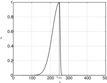
The implementation of the two-step assimilation procedure is represented on Fig. 2. Over the four-day assimilation window, a free run integration of the model is achieved
10
(black curve). The upstream flow correction – correction of the parameters (a,b,c) – is computed using observations from the second and the third days (blue dots). The observation from the first day are not used as the model is potentially not adjusted yet. The resulting analysed parameters are used to correct the upstream flows over the first, second and third days. The updated upstream flows are used for a new
in-15
tegration of the model (starting from the beginning of the four-day window) providing a new integration. This integration (green curve) is intermediate and it describes the background state for the hydraulic state correction procedure. Along the third day of the integration, at each observation time, the water level is adjusted. This correction is instantaneous. The model is integrated starting from the corrected state at an
ob-20
servation time to the next observation time, leading to a discontinuous description of the hydraulic state (discontinuous red curve). In our study, the observation time step is equal to the model time step so that the resulting integration is no more discontinuous than any model integration.
For each cycle, beyond the last observation time, the upstream flows are kept
con-25
HESSD
7, 9067–9121, 2010Data assimilation for flood forecasting
S. Ricci et al.
Title Page
Abstract Introduction
Conclusions References
Tables Figures
◭ ◮
◭ ◮
Back Close
Full Screen / Esc
Printer-friendly Version Interactive Discussion
Discussion
P
a
per
|
Dis
cussion
P
a
per
|
Discussion
P
a
per
|
Discussio
n
P
a
per
|
The data assimilation algorithm is implemented using the PALM (Parallel Assimila-tion with a Lot of Modularity, Lagarde, 2000; Lagarde et al., 2001) dynamic coupler developed at CERFACS. This software was originally developed for the implementa-tion of data assimilaimplementa-tion in oceanography for the use of the MERCATOR project. PALM allows the coupling of independent components with a great modularity in the data
5
exchanges and treatment as well as and easy parallelization environment for the appli-cation (Fouilloux and Piacentini, 1999; Buis et al., 2006).
3 Modeling of B
3.1 Assumptions for the simplification of the hydraulics model
The modeling of the background covariance matrix in the context of the correction of
10
the hydraulic state of MASCARET with data assimilation requires special attention. The modeling of the univariate covariance function inB, i.e. the spatial correlation for the water level on one side and on the discharge on the other side, is investigated here.
Section 3.3 justifies the choice of asymmetric correlation functions at the observation points as opposed to regular gaussian functions. The justification of this approach is
15
made with a simple advection-diffusion model on top of which it was achievable to im-plement a Kalman Filter. Contrary to the BLUE algorithm, the Kalman Filter algorithm explicitly evolves the background error covariances along the cycling of the analysis. It was shown (see Appendix 3.3) that, starting from gaussian correlation functions in the initialB, the Kalman Filter analysis leads to asymmetric covariance functions.
Speci-20
fying such correlation functions with the BLUE algorithm is then equivalent to using a Kalman Filter algorithm. This result was used for the data assimilation hydraulic state correction procedure on MASCARET on top of which it was too costly to implement a Kalman Filter. The correlation lengthl for the correlation function was then estimated assuming the correlation function is gaussian (see Appendix B). Finally, the
correla-25
HESSD
7, 9067–9121, 2010Data assimilation for flood forecasting
S. Ricci et al.
Title Page
Abstract Introduction
Conclusions References
Tables Figures
◭ ◮
◭ ◮
Back Close
Full Screen / Esc
Printer-friendly Version Interactive Discussion
Discussion
P
a
per
|
Dis
cussion
P
a
per
|
Discussion
P
a
per
|
Discussio
n
P
a
per
|
lengthl upstream the observation point and as a gaussian of correlation length l /10 downstream the observation point. The resulting function is local and asymmetric.
Results in Sect. 3.3 (as well as in Appendix A and Appendix B) are based on the crude assumption that the physics of MASCARET can be approximated by the diff u-sive flood approximation equations. Our approach is to assume that the solution of
5
the propagation of a given initial condition by the MASCARET equation is close to the one propagated by the diffusive flood wave approximation equations. More precisely, it is assumed in the following, that the covariance function of a signal (and then its correlation lengthl) propagated by MASCARET is similar to the covariance function of the same signal propagated by the diffusive flood approximation equations. The
ana-10
lytical solution of the MASCARET equations for a given initial condition is usually not known. On the other hand, such solution is known under the flood wave propagation assumption.
In the framework of the diffusive flood wave approximation (S(x,t)=Lh(x,t), where
Lis a constant river width), the diffusive Saint Venant equations Eq. (1) of MASCARET
15
can be crudely approximated by
∂he
∂t+
5Un
3
∂he
∂x =κ
∂2he
∂x2, (19)
whereQ=hU, h=hn+heandU =Un+Ue , with (h,eUe) small perturbations to the equi-librium (hn,Un) and κ=
Unhn
2tanγ for a constant slope γ. The state (hn,Un) such that Un=KsI
1/2
h2n/3is a solution of the flood wave approximation equations, whereI=sinγ.
20
The equilibrium state (hn,Un) for the diffusive flood wave model is chosen as a
repre-sentative mean state for the following simulations with MASCARET on the each catch-ment. Equation (19) is a classical advection-diffusion equation whereκis the diffusion coefficient andc=5Un
3 is the advection speed. To use this model as a support for data
assimilation, an open boundary condition for Eq. (19) is imposed downstream with
25
∂he
∂t(L,t)+c ∂he
HESSD
7, 9067–9121, 2010Data assimilation for flood forecasting
S. Ricci et al.
Title Page
Abstract Introduction
Conclusions References
Tables Figures
◭ ◮
◭ ◮
Back Close
Full Screen / Esc
Printer-friendly Version Interactive Discussion
Discussion
P
a
per
|
Dis
cussion
P
a
per
|
Discussion
P
a
per
|
Discussio
n
P
a
per
|
whereqeis a random function of zero mean<q >=e 0. The auto-correlation function of ˜
q(t)
R(τ)=<qe(t)qe(t+τ)>=δqm2exp −τ
2
2l2
q
!
. (20)
is assumed to be gaussian.
3.2 BLUE algorithm on a 1-D advection-diffusion model
5
To calibrate the data assimilation chain with MASCARET, data assimilation twin ex-periments were set up on the 1-D advection-diffusion model (Eq. 19) with t∈[0,T] and x∈[0,L]. The 1-D domain is discretized in m cells and Eq. (19) is integrated using a Euler explicite scheme in time and an order one centered finite differences scheme in space. A reference run is integrated using the set of parameters and
forc-10
ing (ctrue,κtrue,qetrue(t)) simulating the so called true water level hetrue. The
observa-tion heobs(t)=hetrue(t)+ǫo(t) is calculated at the middle of the 1-D domain (xobs=L2)
where ǫo(t) is a gaussian noise defined by its standard deviation σo. The
back-ground trajectoryhb(x,t) is integrated using a perturbed set of parameters and forcing
(cper,κper,qeper(t)) where<qeper(t)qeper(t+τ)>=δq 2
m,perexp(−τ
2
2l2
q ).
15
The BLUE analysis (Eq. 2) is computed at the subsequent observation timest, as-similating the single observationhobsevery∆t. The background is the water levelhb(x)
at the analysis timet. The analysis at timetis used as the background for the assimila-tion at timet+ ∆t. The observation operator is a column matrix H=(0,...,0,1,0,...,0)T with 1 for thexobs index. The observation error matrix comes down to the scalar
vari-20
ance observation error σo2. The background covariance matrix is a m×m matrix and
HESSD
7, 9067–9121, 2010Data assimilation for flood forecasting
S. Ricci et al.
Title Page
Abstract Introduction
Conclusions References
Tables Figures
◭ ◮
◭ ◮
Back Close
Full Screen / Esc
Printer-friendly Version Interactive Discussion
Discussion
P
a
per
|
Dis
cussion
P
a
per
|
Discussion
P
a
per
|
Discussio
n
P
a
per
|
The spatial correlations inBare represented by the gaussian function
ρ(x,x′)=exp "
−(x−x
′)2
2lB(x,x′)
#
(21)
meaning thatB(x,x′)=σb2ρ(x,x′). The lengthlB(x,x′) is a symmetric function ofxand
x′which represents the local correlation length for the pair (x,x′). For our study, only the correlations ρ(x,xobs) between the errors at xobs and the rest of the domain are
5
relevant. The lengthlB(x,xobs) is estimated as the variance of the impulse response of
the model to a Dirac perturbation ofq(t). This length is first assumed to depend only on the observation point and is denoted byl(xobs).
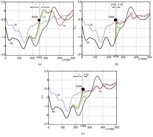
Figure 3(a,b,c) shows the true ˜ht, the non-assimilated ˜hs, background ˜hb and
analysed ˜ha water level state over the 1-D domain at t=T =500×10 3
s when the
10
analysis is performed every ∆t=10×103s, for different functions lB(x,xobs). When
lB(x,xobs)=l(xobs) for allx(Fig. 3a), the data assimilation corrects the water level over the interval [xobs−l(xobs)/2,xobs+l(xobs)/2]. Still, the analysis (red curve) is closer to
the true state (blue dotted curve) than the background (green curve) only upstream the observation point. On the contrary, whenlB(x,xobs)=l(xobs)/10 for allx, on Fig. 3b,
15
the analysis is closer to the true state only downstream the observation point. Finally, as it appears on Fig. 3c, a better fit to the true state is obtained with an asymmetric functionρ(x,xobs) with
l−=lB(x,xobs)= l(xobs) whenx < xobs,
l+=lB(x,xobs)=l(xobs)/10 whenx > xobs.
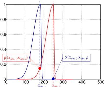
(22) The choice of an asymmetric correlation function described by Eq. (22) is quite
un-20
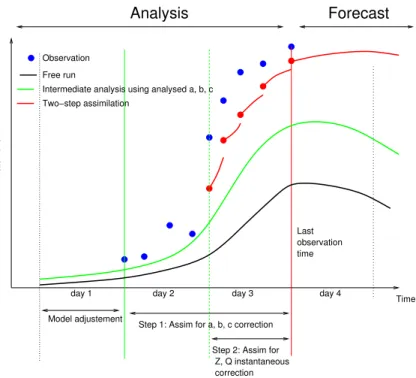
usual and should be treated carefully as it might lead to a non symmetric B matrix erroneous setting. Indeed, with an asymmetric correlation function, considering for in-stance two nearby observation pointsxobs,1,xobs,2withl(xobs,1)=l(xobs,2) would imply
thatρ(xobs,1,xobs,2)6=ρ(xobs,2,xobs,1) as drawn on Fig. 4. In this case, this falls down to
B(x1,x2)6=B(x2,x1) andBis not symmetric.
HESSD
7, 9067–9121, 2010Data assimilation for flood forecasting
S. Ricci et al.
Title Page
Abstract Introduction
Conclusions References
Tables Figures
◭ ◮
◭ ◮
Back Close
Full Screen / Esc
Printer-friendly Version Interactive Discussion
Discussion
P
a
per
|
Dis
cussion
P
a
per
|
Discussion
P
a
per
|
Discussio
n
P
a
per
|
It appears that the asumption of asymmetric correlation functions must go along with the asumption of local correlation lengths so that the relationlB(x1,x2)=lB(x2,x1)
remains true and B(x1,x2)=B(x2,x1) remains true. The definition from Eq. (22) is
thus only valid if there is only one observation point or if the observation points are separated by sufficiently large distances.
5
It should be mentioned that in our examples the matrix B is not fully formulated. Only the columnB(x,xobs) is used, meaning that onlyρ(x,xobs) andσ
2
b(xobs) should be
explicitely modeled. Since B(xobs,x) is never formulated, along with ρ(xobs,x), there
is no need to question the symmetry of the B matrix. In the case of the MASCARET application, there are several observation points but they are far enough from each
10
other for us to assume that there is no spatial correlations between two observation points. Each observation point is treated independently of the others.
3.3 Modeling of the background error spatial correlations
The Kalman Filter algorithm is now implemented on the 1-D advection-diffusion model described by Eq. (19), using the same twin-obs framework as previously described.
15
In this context, the background error covariance matrix is updated by the analysis and propagated in time by the tangent linear of the model (Eqs. 10–11). As a consequence, the gain matrix evolves over the assimilation cycle (Eq. 9). A detailed explanation of the evolution of the covariance function at the observation point as well as at an upstream and a downstream location are presented in Appendix along with illustrations.
20
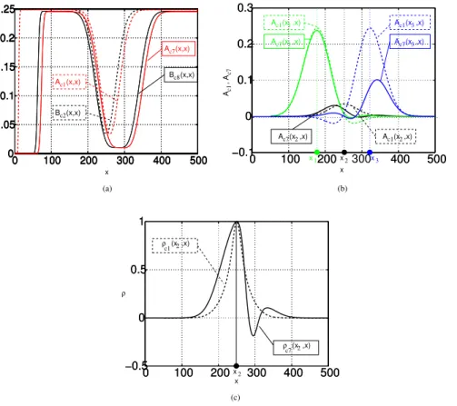
Initially, the background covariance matrix is modeled by spatially constant variances and correlation length for a gaussian correlation function. After the first assimilation cy-cle, the error covariances are locally modified. The analysis error covariance matrix is computed from Eq. (10). The analysis error at the observation point is reduced. At upstream and downstream points, the covariance function are asymmetric. The
covari-25
HESSD
7, 9067–9121, 2010Data assimilation for flood forecasting
S. Ricci et al.
Title Page
Abstract Introduction
Conclusions References
Tables Figures
◭ ◮
◭ ◮
Back Close
Full Screen / Esc
Printer-friendly Version Interactive Discussion
Discussion
P
a
per
|
Dis
cussion
P
a
per
|
Discussion
P
a
per
|
Discussio
n
P
a
per
|
cycle results from the propagation of the previous cycle analysis error covariance ma-trix by the tangent linear of the modelMand its adjointMT as formulated in Eq. (11). The initially prescribed symmetric correlation function at the observation pointx2 has
been modified into a local and asymmetric function. At the observation pointx2, the
correlation function is asymmetric with a shorter correlation length downstream than
5
upstream.
The application of a complete Kalman Filter on this simple advection-diffusion model enabled the understanding of the impact of the analysis and the physics on initial gaus-sian correlation function. It was explained (see Appendix A) how the information at the observation point leads to the reduction of the uncertainty at the observation point and
10
then downstream this location. It was also explained how the correlation length scale is reduced downstream the observation point and how the initial gaussian correlation function evolves into an asymmetric correlation function. For the MASCARET applica-tion, the implementation of a complete Kalman Filter is not possible, mostly because of the high computing cost of the estimation and propagation of the tangent linear model
15
(and it’s adjoint). Still, the results presented here on the 1-D advection-diffusion model were used to model the correlation function for water level and discharge in the MAS-CARET data assimilation procedure. An approximate reduction factor of ten was taken between correlation lengths upstream and downtream the observation points, this di-vision factor showed better results then the factor actually deduced from the Kalman
20
Filter study on the 1-D advection-diffusion model.
In order to finalize to modeling of the background error covariance function, the value of the correlation lengthl(xobs) must then be estimated. Our objective here is to
deter-mine the correlation length of the spatial correlation function for the errors on the water level and the discharge errors with MASCARET. This determination is two-fold. First a
25
HESSD
7, 9067–9121, 2010Data assimilation for flood forecasting
S. Ricci et al.
Title Page
Abstract Introduction
Conclusions References
Tables Figures
◭ ◮
◭ ◮
Back Close
Full Screen / Esc
Printer-friendly Version Interactive Discussion
Discussion
P
a
per
|
Dis
cussion
P
a
per
|
Discussion
P
a
per
|
Discussio
n
P
a
per
|
in the following to prescribe the correlation length at each observation point for the data assimilation in MASCARET as described in Eq. (22), defining the spatial corre-lation function along the 1-D discretized domain. The steps for the estimation of the correlation lengthl(xobs) are given in Appendix B.
4 Results of the data assimilation on the Adour catchment
5
4.1 Description of the catchments
The data assimilation study is applied on the Adour maritime catchment area as well as on the Marne Vallage area. A description of theses catchments is given in Sect. 4.1.1 and Sect. 4.1.2, respectively.
4.1.1 Description of the adour catchment
10
The Adour maritime catchment area is located in Southwestern france, from the Pyre-nean Piedmont to the Aquitain coast. This 16 890 km2 drainage area estuary lies on two departements (Atlanitic Pyr ´en ´ees and Landes). The Adour river rises in the Pyre-nees at an altitude of 2600 m and reaches the Atlantic ocean in Bayonne 312 km fur-ther. The Adour catchment is one of the wettest in France due to strong precipitations
15
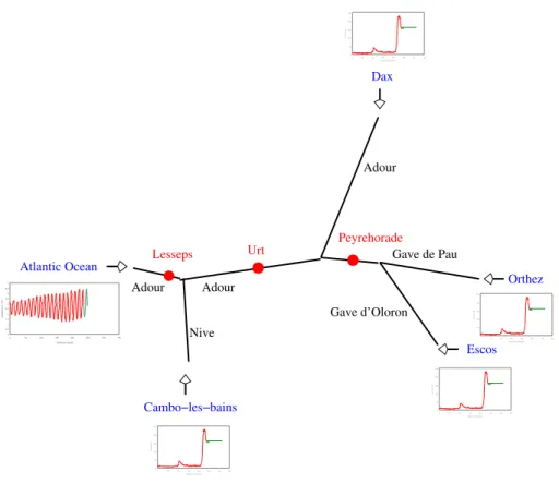
in the upper part of the basin. The Adour catchment is divided in two regions: the mouth of the river mostly influenced by the tide and the upstream region mostly influ-enced by the affluents. A schematic description of the Adour catchment is shown on Fig. 7.
The Adour river has three main affluents (responsible for 65% of the total discharge
20
in Bayonne in flood conditions). The Gaves de Pau et d’Oloron, respectivly draining 5226 km2 and 608 km2, are often affected by flash floods and gather into the main affluent of the catchment named Gave R ´eunis. The Nive drains 980 km2 and joins up with the Adour close to Bayonne. The catchment area is limited by three thresholds controlling the tide waves propagation (at the Gave d’Oloron, Gave de Pau and Nive).
HESSD
7, 9067–9121, 2010Data assimilation for flood forecasting
S. Ricci et al.
Title Page
Abstract Introduction
Conclusions References
Tables Figures
◭ ◮
◭ ◮
Back Close
Full Screen / Esc
Printer-friendly Version Interactive Discussion
Discussion
P
a
per
|
Dis
cussion
P
a
per
|
Discussion
P
a
per
|
Discussio
n
P
a
per
|
The upstream affluents flow in a mountainous region and their flood plain is narrow. The riverbed becomes larger as the hillslopes decrease. The river banks are partly equiped and the overflowing is stored by embankment dykes allowing the control of the Adour floods.
Meteorological data are provided by Meteo-France. They provide pressure at sea,
5
pressure at land (Biarritz airfield), wind direction and intensity as well as water level anomaly at the coast (these are not used in the MASCARET simulation). The hydro-logic (water level and corresponding discharge) data are available in real time at the SPC2 upstream stations: Dax, Escos, Orthez and Cambo-les-bains and are used as discharge boundary conditions for the hydraulics model. The maritime boundary
con-10
ditions are given by the SPC tide gauge located in the estuary. Tide forecast are given by the SHOM3. Additionally, tide gauges located at Lesseps, Urt and Peyrehorade sta-tions display the water level every five minutes or hourly. These last observasta-tions are used for the data assimilation process. The water level at the river mouth varies be-tween 0.9 m and 4.55 m on a semi-diurnal cycle coupled with a bi-weekly signal. Tide
15
waves time propagation ranges between one hour at Lesseps and four hours at Dax for high-tide conditions.
The MASCARET model was chosen by the SCHAPI4to simulate the physics of the Adour catchment. A preliminary calibration procedure of several model parameters was done by the SCHAPI using data from twelve flood events of varying intensity.
20
The geometry of the hydraulic network, the computation time step and the Strickler coefficient were ajusted so that the tide and the flood events are well represented at Urt, Dax, Lesseps and Peyrehorade. Globally, at Peyrehorade, the simulation tends to overestimate the flood peak for big flood events and underestimate the flood peak for moderate events.
25
2
Service de Pr ´evision des Crues
3
Service Hydrographique et Oc ´eanographique de la Marine
4
HESSD
7, 9067–9121, 2010Data assimilation for flood forecasting
S. Ricci et al.
Title Page
Abstract Introduction
Conclusions References
Tables Figures
◭ ◮
◭ ◮
Back Close
Full Screen / Esc
Printer-friendly Version Interactive Discussion
Discussion
P
a
per
|
Dis
cussion
P
a
per
|
Discussion
P
a
per
|
Discussio
n
P
a
per
|
4.1.2 Description of the marne catchment
The Marne Vallage catchment is located East of the Paris basin. The Marne river is the main affluent of the Seine river and is 525 km long. The Marne catchment area is divided in three main regions: two separated regions upstream the Lac de Der (Marne Amont and Marne Vallage) and one region downstream the Lac de Der (Marne
5
Moyenne). Our study focuses the Marne Vallage drainage area that lies between Con-des and Chamouilley.
The Marne river has two main affluents. The Rognon is responsible for 50% of the Marne discharge. This karstic basin is caracterised by slow flood rises, long flooding period and strong sensibility to local precipitations. The Rongeant is a calcareous
10
basin and has a strong reactivity to precipitation. The Marne Vallage catchment is divided in three regions: upstream the Rognon/Marne confluence between Condes and the confluence, upstream the Rognon/Marne confluence between Saucourt and the confluence and downstream the Rognon/Marne confluence between Chamouilley and the Rognon/Marne confluence. A schematic description of the Marne Vallage
15
catchment is shown on Fig. 8.
The hydrologic data are provided by the Champagne-Ardenne DIREN at Con-des, Saucourt, Joinville and Chamouilley. The hourly observations at Joinville and Chamouilley are used for the data assimilation procedure. There are two upstream boundary condition (Saucourt and Condes) described by hydrograms and one
down-20
stream boundary condition described by a rating curve (correlation between water level and dischage).
As for the Adour catchment, the MASCARET model was chosen by the SCHAPI to simulate the physics of the Marne Vallage catchment. A preliminary calibration pro-cedure of several model parameters was done by the SPC Seine-aval Marne-amont
25
HESSD
7, 9067–9121, 2010Data assimilation for flood forecasting
S. Ricci et al.
Title Page
Abstract Introduction
Conclusions References
Tables Figures
◭ ◮
◭ ◮
Back Close
Full Screen / Esc
Printer-friendly Version Interactive Discussion
Discussion
P
a
per
|
Dis
cussion
P
a
per
|
Discussion
P
a
per
|
Discussio
n
P
a
per
|
simulated at Joinville are globally correct, though often overestimated and the flood peak is often underestimated at Chamouilley.
4.2 Data assimilation set-up
The two-step assimilation procedure described in Sect. 2.3.3 is applied on the Adour catchment and on the Marne Vallage catchment for several flood events. For the Marne
5
catchment, illustrations are shown for an episode in April 2006 (starting 03/23/2006) with a single flood peak. For the Adour catchment, illustrations are shown for an episode in November 2002 (starting 11/02/2002) with a single flood peak as well as for an episode in November 2009 (starting 11/09/2009) with two flood peaks. Statistics are computed over five episodes between 2002 and 2004 for which the observations
10
are hourly (for the 2009 event, the observations are available every five minutes). For the Marne Vallage catchment, the downstream boundary condition is not con-sidered in the control. Using Eq. (16) and considering the Marne Vallage catchment’s two free extremities, the size of the control vector is equal to six. Sensitivy tests at each free extremity for the Marne Vallage catchment revealed that the tangent linear
15
model is valid for a pertubation up to 20% ona, 6 m3s−1onband 6 h onc. For the hy-draulic state correction approach, the correlation length were set using the procedure described in Sect. 3, to 51 km and 55 km at Joinville and Chamouilley, respectively.
For the Adour catchment, the oceanic upstream water level is not considered in the control since the uncertainty on the maritime boundary condition is smaller than that
20
of the other free extremities (no use of a rating curve). Using Eq. (16) and considering the Adour catchment’s four free extremities, the size of the control vector is equal to twelve. Sensitivity tests at each free extremity for the Adour catchment revealed that the tangent linear model is valid for a pertubation up to 20% ona, 20 m3s−1 onband 6 h onc. For the hydraulic state correction approach, the correlation length were set
25
HESSD
7, 9067–9121, 2010Data assimilation for flood forecasting
S. Ricci et al.
Title Page
Abstract Introduction
Conclusions References
Tables Figures
◭ ◮
◭ ◮
Back Close
Full Screen / Esc
Printer-friendly Version Interactive Discussion
Discussion
P
a
per
|
Dis
cussion
P
a
per
|
Discussion
P
a
per
|
Discussio
n
P
a
per
|
Hydraulic observations are gathered in the FrenchBanque Hydrodata base5. River gauges and tide gauges give an approximate and incomplete description of the water level in space and time. The quality of these data greatly relies on the quality of the measurement and for some of them is better in low water conditions then in flood conditions. Additionally, discharge observations are usually derived from water level
5
measurements using a calibration procedure that could be questionned.
In our study, the observed water level reaches up to a couple of meters and the observation error standard deviations are prescribed to 0.1 m. The observation er-ror covariances are neglected assuming that the observations stations are far enough for the spatial errors to be weakly correlated. The background error variances were
10
chosen two to three times bigger than the observation error variances. At each obser-vation point, only the obserobser-vations above a minimal value are taken into account for the assimilation process to avoid representativeness errors. Additionaly, a threshold is ap-plied on the misfit between the observation and the simulated water level to eliminate inconsistent observations.
15
4.3 Illustration of the data assimilation method
Figure 9 shows the water level over a four-day period (Day 19 to Day 22 of a flood event in November 2002) at the observation station at Peyrehorade on the Adour catchment. The integration of MASCARET (free run) starting from a previously calculated state is plotted in black and the hourly observations are plotted in blue. The difference between
20
these two curves reaches 15% of the observation at the beginning of Day 22. The assimilation procedure is applied to improve the water level over the first three days (re-analysis period) as well as over a so-calledforecastperiod (Day 22). The anaysis with the instantaneous correction of the water level (purple curve) shows an excellent fit to the observations over the re-analysis period but to a minor improvement over
25
the forecats period. The model is constantly constrained to the observed state by
5
HESSD
7, 9067–9121, 2010Data assimilation for flood forecasting
S. Ricci et al.
Title Page
Abstract Introduction
Conclusions References
Tables Figures
◭ ◮
◭ ◮
Back Close
Full Screen / Esc
Printer-friendly Version Interactive Discussion
Discussion
P
a
per
|
Dis
cussion
P
a
per
|
Discussion
P
a
per
|
Discussio
n
P
a
per
|
the hydraulic state correction procedure from Day 19 to Day 22. Even though the analysed state is almost egal to the observed state at the beginning of Day 22, over the forecast period, the analysis remains far from the observation. This shows that the improvement of the initial conditon at Day 22 is not enough to improve the simulation over the following day. The improvement is only significant over a couple of hours and
5
other uncertainties degrade the simulation. Effectively, the upstream flow is known up to Day 22 and is kept constant over the forecast period. The analysis after the correction of the upstream flow (green curve) shows a good fit to the observation over the past period as well as over the forecast period. The difference to the observation only reaches 9% of the observed value at Day 22.5. The upstream flow is corrected
10
over the two-day period (Day 20 to Day 22) allowing for a better simulation of the water level over this period. Additionally, over the forecast period, the upstream flow is kept constant to the last analysed value (which is obviously better than the non-analysed one) allowing for a significant improvement of the water level over Day 22. The analysis after the two-step assimilation procedure is plotted in red and shows an improvement
15
over the re-analysis as well as over the forecast period.
For this event, the two-step analysis is cycled every hour so that, at an observation point, the water level is forecasted over the whole flood event. Figure 10 shows the six-hour forecast for the free (black curve) and the assimilated runs (red curve) as well as the non assimilated observations (blue curve). It clearly appears that the assimilation
20
improves the six-hour forecast. Shorter and longer ranges for the forecast were also studied leading to similar conclusions.
Similar representation is provided on Fig. 11 for the November 2009 event on the Adour catchment. Observations at the previously described stations are available ev-ery five minutes. The non assimilated observation (forecast mode) are represented
25
HESSD
7, 9067–9121, 2010Data assimilation for flood forecasting
S. Ricci et al.
Title Page
Abstract Introduction
Conclusions References
Tables Figures
◭ ◮
◭ ◮
Back Close
Full Screen / Esc
Printer-friendly Version Interactive Discussion
Discussion
P
a
per
|
Dis
cussion
P
a
per
|
Discussion
P
a
per
|
Discussio
n
P
a
per
|
correctly represented eventhough the flood rise is too slow. The two-step data assim-ilation (red curve) enables the exact representation of the both flood peaks as well as a more realistic flood rise for the second peak. Same results were observed at the other observation stations.
Finally, the two-hour and the seven-hour forecasted water level on the Marne Vallage
5
catchment, for the April 2006 event is presented on Figs. 12 and 13, respectively. The free run simulation significantly overestimates the flood peak at Joinville and Chamouil-ley (not shown) and the two-step data assimilation procedure allows for a good simu-lation of the peak at a two-hour forecast. The simulated peak at seven-hour forecast is also in better agreement with the observations than the free run, even though an
10
overestimation of the peak remains. More analysis were carried out for flood events on the Marne Vallage catchment. Globally, the results are not as satysfing as on the Adour catchment. The main reason for this moderated performance is an incomplete and perfectible calibration of the numerical model (mostly Strickler coefficient and lat-eral input flow) on the Marne Vallage catchment before the assimilation procedure. It
15
was shown on some events, that in order to improve the simulation at one observation station, the data assimilation algorithm must degradate the simulation at the other ob-servation location. The application of the two-step data assimilation procedure enabled the detection of a model incoherence on the Marne Vallage that can not be efficiently accounted for with the present control vector. Further work towards the improvement
20
of the calibration of the model for the Marne Vallage catchment is ongoing at the SPC Seine-aval Marne-amont and will be used with the data assimilation procedure when available.
4.4 Interpretation of the results
4.4.1 Criteria for the interpretation
25
HESSD
7, 9067–9121, 2010Data assimilation for flood forecasting
S. Ricci et al.
Title Page
Abstract Introduction
Conclusions References
Tables Figures
◭ ◮
◭ ◮
Back Close
Full Screen / Esc
Printer-friendly Version Interactive Discussion
Discussion
P
a
per
|
Dis
cussion
P
a
per
|
Discussion
P
a
per
|
Discussio
n
P
a
per
|
to estimate the impact of the analysis on the water level simulation at each observation point.
We present here the computation of the standard deviation of the difference between the Free run and the Observation at an observation point for the water level, denoted by FmO (Free run Minus Observation, in m), and the difference between the Analysis
5
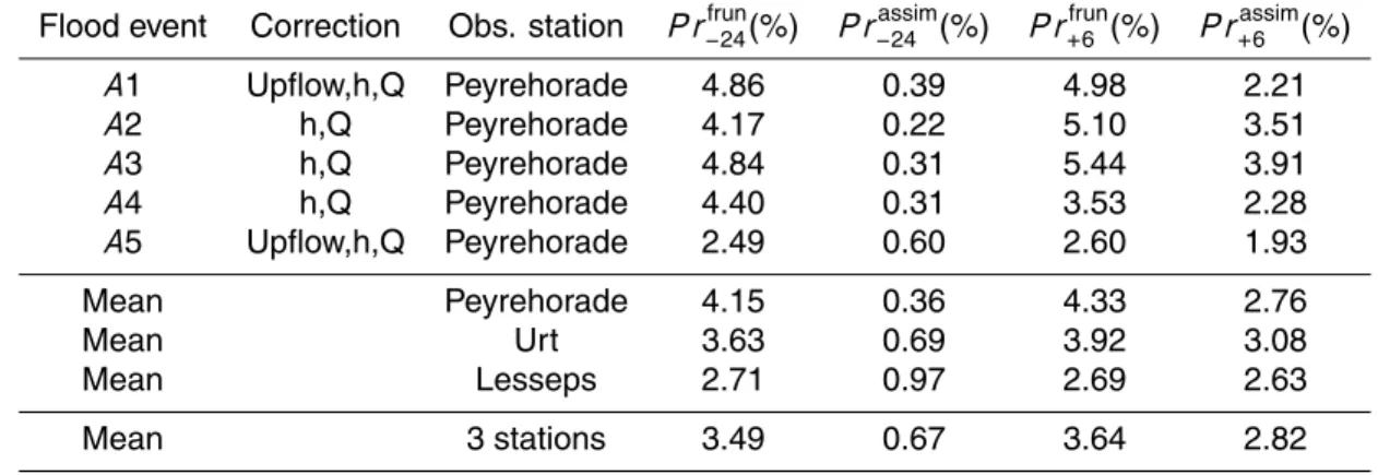
and the Observation, denoted by AmO (Analysis Minus Observation, in m). These differences are computed for a given forecast range (six-hour in our case) at each observation time (one hour or five minutes). The standard deviation is computed over time for each flood event as well as over the simulated flood events. The precision criteriaP r (in %) is also defined as
10
P r= 100
Nobs
Nobs
X
1
|h
mod
−hobs
hobs |, (23)
whereNobs is the number of observations over a period (24 h in re-analysis mode and
six hours in forecast mode in our case) andhmod is the simulated water level with or without the assimilation. When computed with the free run simulation, the precision is notedP rfrun whereas when computed with the analysed water level, the precision is
15
notedP rassim.
It must be noted that the assimilation procedure is not the same for every flood event. In some cases, because of the model instabilitiy (more precisely of its use on the Adour catchment), it was not possible to achieve the free run with MASCARET over a two-day period used as the background for the data assimilation procedure, it was
20