Effect of Spatial Dispersion on Evolutionary Stability: A Two-Phenotype and Two-Patch Model.

Effect of Spatial Dispersion on Evolutionary

Stability: A Two-Phenotype and Two-Patch

Model

Qing Li1, Jiahua Zhang2, Boyu Zhang3*, Ross Cressman4, Yi Tao2

1School of Mathematical Sciences, Capital Normal University, Beijing, China,2Key Lab of Animal Ecology and Conservational Biology, Institute of Zoology, Chinese Academy of Sciences, Beijing, China,3Laboratory of Mathematics and Complex Systems, Ministry of Education, School of Mathematical Sciences, Beijing Normal University, Beijing, China,4Department of Mathematics, Wilfrid Laurier University, Waterloo, ON, Canada

*zhangby@bnu.edu.cn

Abstract

In this paper, we investigate a simple two-phenotype and two-patch model that incorporates both spatial dispersion and density effects in the evolutionary game dynamics. The migra-tion rates from one patch to another are considered to be patch-dependent but independent of individual’s phenotype. Our main goal is to reveal the dynamical properties of the evolu-tionary game in a heterogeneous patchy environment. By analyzing the equilibria and their stabilities, we find that the dynamical behavior of the evolutionary game dynamics could be very complicated. Numerical analysis shows that the simple model can have twelve equilib-ria where four of them are stable. This implies that spatial dispersion can significantly com-plicate the evolutionary game, and the evolutionary outcome in a patchy environment should depend sensitively on the initial state of the patches.

Introduction

In order to explain the evolution of animal behavior, Maynard Smith and Price [1] developed the concept of evolutionarily stable strategy (ESS) (see also [2–5]). Prior et al. [6] investigated an evolutionary game model that incorporates both spatial dispersion and density effects in the evolutionary dynamics. In this model, the population is considered to be dispersed in a patchy environment, where the background fitness and payoff matrix in each patch can be different. Migration from region to region is considered as an incidental aspect of the population, i.e., the migration is a chance event unrelated to an individual’s phenotype (strategy) or the fitness of the patch. As pointed out by Prior et al. [6], their assumptions differ from that of Ludwig and Levin [7] who treat the tendency to migrate as an individual characteristic subject to selection (see also [8–13]), and also differ from that of Hines and Maynard Smith [14] who interpret the effect of spatial dispersion as an increased tendency to interact with opponents sharing one’s own characteristics (see also [15]). Recently, Cressman and Krivan [16] investigated the migra-tion dynamics for the ideal free distribumigra-tion (IFD) in a patchy environment. They showed that OPEN ACCESS

Citation:Li Q, Zhang J, Zhang B, Cressman R, Tao Y (2015) Effect of Spatial Dispersion on Evolutionary Stability: A Two-Phenotype and Two-Patch Model. PLoS ONE 10(11): e0142929. doi:10.1371/journal. pone.0142929

Editor:Gui-Quan Sun, Shanxi University, CHINA

Received:July 2, 2015

Accepted:October 27, 2015

Published:November 13, 2015

Copyright:© 2015 Li et al. This is an open access article distributed under the terms of theCreative Commons Attribution License, which permits unrestricted use, distribution, and reproduction in any medium, provided the original author and source are credited.

Data Availability Statement:All relevant data are within the paper.

Funding:This work was supported by National Natural Science Foundation of China, No. 11471221, No. 11301032 and No. 31270439 (http://www.nsfc. gov.cn/);“the Fundamental Research Funds for the Central Universities”of China (http://www.gov.cn/); and Natural Science Foundation of Beijing Municipal. No. 1132003 (http://www.bjnsf.org/). The funders had no role in study design, data collection and analysis, decision to publish, or preparation of the manuscript.

IFD is evolutionarily stable under the assumptions that individuals never migrate from patches with a higher payoff to patches with a lower payoff and some individuals always migrate to the best patch. But migration does not necessarily lead to IFD if migration rates are independent of the payoffs of the patches.

For the evolutionary game dynamics in a patchy environment, Prior et al. [6] mainly focused their analysis on the stability of the homogeneous states, where they assumed that all patches have the same payoff matrix and density-dependent background fitness. Their main results showed that a stable equilibrium (e.g. an evolutionarily stable strategy) of the non-dis-persed frequency dynamics becomes a stable equilibrium of the large system if population den-sity stabilizes at these fixed frequencies.

In this paper, following Prior et al. [6], a simple two-patch and two-phenotype model is investigated. Three basic assumptions for this model are:

(i) The environment consists of two patches, called patch 1 and patch 2, respectively. Individu-als can move from one patch to the other at any timet. The migration rates are patch-dependent but inpatch-dependent of individual’s phenotype [6]. Letc1denote the probability that an individual moves from patch 1 to patch 2, and, similarly,c2the probability that an indi-vidual moves from patch 2 to patch 1.

(ii) In each of two patches, individuals display two possible phenotypes (strategies), denoted byR1andR2, and individuals interact in random pairwise contests. The payoff matrix is

A_¼ a11 a12

a21 a22 !

in patch 1 andB_¼ b11 b12

b21 b22 !

in patch 2, whereaij(orbij) is the

pay-off of an individual displaying phenotypeRiwhen it plays against an individual displaying phenotypeRjin patch 1 (or in patch 2) for alli,j= 1, 2. Without loss of generality, we also assume thataij0 andbij0 for alli,j= 1, 2.

(iii) In each of the two patches, the background fitness is density-dependent [3–4], which is defined asα₁−β1n1in patch 1, andα2−β2n2in patch 2, wheren1is the total population size in patch 1 andn2the total population size in patch 2. We also assume thatα_i>cifor all i= 1, 2. That is, the migration rates are small enough to ensure that population size in a patch will increase when there are few individuals in the patch.

Letxidenote the number of individuals with phenotypeRiin patch 1, andyithe number of individuals with phenotypeRiin patch 2 (i= 1, 2). Clearly,n1=x1+x2andn2=y1+y2. Simi-larly, letpdenote the frequency of phenotypeR1in patch 1, andqthe frequency of phenotype R1in patch 2, i.e.,p=x1/n1andq=y1/n2. According to the basic assumption (ii), the expected payoff of an individual displaying phenotypeRiisfi=pai1+ (1−p)ai2in patch 1, andgi=qbi1 + (1−q)bi2in patch 2 fori= 1, 2. Similarly, according to the basic assumption (iii), the (total) fitness of an individual displaying phenotypeRiis defined asFi= (α₁−β1n1) +fiin patch 1, andGi= (α₂−β2n2) +giin patch 2 fori= 1, 2. Thus, the time evolution ofxiandyican be given by

dxi

dt ¼

½

Š

dyi

dt ¼

½

Š

ð1Þ

respectively, fori= 1, 2. Dynamics (1) also equivalent to the following system expressed in

terms of phenotypic frequency and population size in each patch.

dp

dt ¼pð1 pÞðf1 f2Þ þc2ðq pÞ n2 n1 ;

dq

dt ¼qð1 qÞðg1 g2Þ þc1ðp qÞ n1 n2 ;

dn1 dt ¼

½

f þða1 b1n1Þ

Š

dn2

dt ¼

½

Š

ð2Þ

wheref ¼pf1þ ð1 _{pÞf2andg¼qg1þ ð}1 _{qÞg2are the average payoffs in patch 1 and} patch 2, respectively.

In this paper, the equilibria of dynamics (2) and their stabilities are analyzed. Different from Prior et al. [6] who focused on the homogeneous states, we are primarily interested in analyzing the heterogeneous states, where two patches have different ESSs. Our main goal is to reveal the dynamical properties of the evolutionary game in a heterogeneous patchy environment.

Results

Symmetric equilibria of dynamics (2)

For givenpandqwith 0p,q1, an equilibrium of dynamics

dn1 dt ¼n1

f þða1 b1n1Þ

c1n1þc2n2 ;

dn2

dt ¼n2ðgþða2 b2n2ÞÞ c2n2þc1n1 ;

ð3Þ

denoted by (n1(p,q),n2(p,q)), satisfies n2¼n1

c2 c1

f ða1 b1n1Þ

;

n1¼n2

c1ðc2 g ða2 b2n2ÞÞ :

ð4Þ

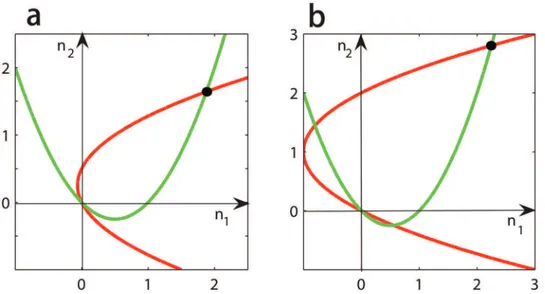
It is clear that (n1,n2) = (0, 0) is always a solution ofEq (4)for any givenpandq. Furthermore, (p,q, 0, 0) must be unstable under dynamics (2) sinceα₁>c1andα₂>c2. Notice thatn2is a parabolic function ofn1and vice versa,Eq (4)also has a unique positive solution, denoted by ð^_n1;n2^_{Þ ¼ ðn1ðp;qÞ;n2ðp;qÞÞwith}^_n1>0_andn2^ _>0_{(seeFig 1). When this solution} corre-sponds to an equilibriumðp;q;^_n1;n2^_{Þof dynamics (2), we call it apositiveequilibrium. In the} rest of this paper, we only focus on the number and stabilities of these positive equilibria.

A positive equilibrium,ðp;q;^_n1;n2^_{Þ, is called asymmetricequilibrium of dynamics (2) ifp=} q. That is, at a symmetric equilibrium, population compositions in the two patches are the same.

It is easy to see that dynamics (2) always have two symmetric boundary equilibria,

ð1_;1_;n1^_;n2^_Þandð0_;0_;n1^_;n2^_{Þ, where at these equilibria, all individuals in the two patches} dis-play the same phenotype. Stabilities of the boundary equilibria can be characterized by analyzing the Jacobian matrix of dynamics (2) (seeMethodsection). The main result is that ifR1(orR2) is an ESS for both payoff matricesAandB, then the boundary equilibriumð1_;1_;^_n1;n2^_Þ(or

where the stable equilibrium of the non-dispersed system becomes a stable equilibrium of dynam-ics (2). However, under the influence of migration, a symmetric boundary equilibria could be sta-ble even if the corresponding phenotype is not an ESS in either patch. For instance, the boundary equilibriumð1_;1_;n1^_;n2^_{Þis asymptotically stable ifa11<a21as long asa21−a11is small enough.} On the other hand, the symmetric interior equilibrium exists only for a very special casep =q_{2(0, 1), wherep¼} a12 a22

a12 a22þa21 a11andq

_¼ b12 b22

b12 b22þb21 b11. In this case,ðp

_{;q;n1^;n2^Þis an}

symmetric interior equilibrium of dynamics (2), whereð^_n1;n2^_{Þis the solution ofEq (4)forp=} p_{andq=q. Furthermore, it is asymptotically stable ifp(=q) is an ESS for bothAandB} (seeMethodsection).

General cases

For more general situations (i.e.,p6¼q), it is very tedious to determine the equilibria of dynamics (2). In fact, numerical simulations show that dynamics (2) may have twelve equilib-ria. To investigate the properties of the equilibria of dynamics (2), two cases are considered below. The first case is special in that there is no migration in one direction (i.e., one ofc1and c2is 0) and we analyze the number of stable equilibria for all possible payoff structures. The second case is more general (i.e.,c1>0 andc2>0) and we show the equilibria of dynamics (2) and their stabilities for 0<p,q<1.

Case 1.c1>0andc2= 0. Without loss of generality, we here assume thatc1>0 butc2= 0, i.e. individuals can only move from patch 1 to patch 2 but not from patch 2 to patch 1 (the case ofc1= 0 andc2>0 can be analyzed analogously). Then, dynamics (2) can be rewritten as

dp

dt ¼pð1 pÞðf1 f2Þ ;

dn1

dt ¼ a1þ

_{f c1 b1n1}

n1 ;

ð5Þ

Fig 1. The unique positive equilibrium of dynamics (3).The red curves correspond to the second equation ofEq (4)and the green curves to the first equation ofEq (4). For any givenpandq, the two curves have a unique positive intersection (see the black spots). Parameters are taken asβ1=β2= 0.01,α1= 0.75,

f ¼0_:25_{,c1= 0.5 andc2= 0.5 in all two panels. Furthermore,α2= 0.55 andg¼}0_:2_{in panela, andα2= 1 and}

g¼0_:5_{in panelb.}

doi:10.1371/journal.pone.0142929.g001

and

dq

dt ¼qð1 qÞðg1 g2Þ þc1ðp qÞ n1 n2;

dn2

dt ¼ða2þg b2n2Þn2þc1n1 :

ð6Þ

Notice that dynamics (5) is independent of dynamics (6). Thus, as an equilibrium of dynam-ics (2),ð^_p;q^_;^_n1;n2^_{Þ, is locally asymptotically stable if and only ifð}^_p;n1^_{Þis locally} asymptoti-cally stable under dynamics (5) andð^_q;n2^_{Þis locally asymptotically stable under dynamics (6),} wherepandn1in dynamics (6) correspond to the stable equilibrium,ð^_p;n1^_{Þ, of dynamics (5).}

We first look at the stability of dynamics (5). It is easy to see that: (i) the boundary equilib-riumð1_;^_n1Þ(orð0_;n1^_{Þ) is locally asymptotically stable if and only ifp= 1 (orp= 0) is an ESS} for the payoff matrixA, i.e.a11>a12(ora22>a12), where^_{n1 ¼}a1þa11 c1

b1 forp= 1 andn1^ ¼ a1þa22 c1

b1 forp= 0; and (ii) if the unique interior equilibriumðp

_;n1^_{Þexists, then it is globally}

asymptotically stable if and only ifp_{is an ESS for the payoff matrixA, wherep ¼} a12 a22

a12 a22þa21 a112 ð

0_;1_Þandn1^ _¼a1þfðpÞ c1 b1 .

From dynamics (6), the frequency_q^_{in a stable equilibrium of dynamics (2),ðp}^_;q^_;n1^_;n2^_Þ, should obey the equation

qð1 _{qÞðg1 g2Þ þ} ^

p q

2

ffiffiffiffiffiffiffiffiffiffiffiffiffiffiffiffiffiffiffiffiffiffiffiffiffiffiffiffiffiffiffiffiffiffiffiffiffiffiffi

ða2þ_gÞ2_þ4_b2c1n1^ q

ða2þ_gÞ

¼ 0_{; ð7Þ}

where_p^_{2 f}0_;1_{;pgcorresponds to the stable equilibrium,ðp}^_;n1^_{Þ, of dynamics (5). In the} Method section, we analyze the solutions ofEq (7)and the stabilities of the corresponding equilibria under dynamics (6). According to the stability conditions of dynamics (5) and (6), the equilibria of dynamics (2) and their properties can be summarized as follows:

1. IfR1(orR2) is the only ESS forAandB, then the symmetric boundary equilibrium ð0_;0_;^_n1;^_n2Þ(orð1_;1_;n^_1;n^_{2Þ) is unstable and the otherð}1_;1_;^_n1;n^_2Þ(orð0_;0_;n^_1;^_{n2Þ) is} stable. Furthermore,Eq (7)has no interior solution. This implies thatð1_;1_;^_n1;n^2Þ(or

ð0_;0_;^_n1;^_{n2Þ) is also globally asymptotically stable, i.e., all individuals in the two patches will} eventually displayR1(orR2) under evolutionary dynamics (2) (seeFig 2A and 2B).

2. If bothR1andR2are ESSs forAbutR1(orR2) is the only ESS forB, then the symmetric boundary equilibriumð0_;0_;n^1;n^2Þ(orð1;1;n^1;^n2Þ) is unstable and the otherð1;1;^n1;^n2Þ (orð0_;0_;^_n1;n^_{2Þ) is stable. Furthermore,Eq (7)has a unique (interior) solution}^_{q, which} corresponds to an asymptotically stable equilibriumð0_;q^_;n^1;^n2Þ(orð1;^q;^n1;^n2Þ) of dynamics (2). In this situation, either all individuals in the system displayR1(orR2), or individuals in patch 1 displayR2(orR1) and two phenotypes coexist in patch 2 (seeFig 2C and 2D).

3. Ifp_{is the only ESS forA(0<p<1) andR1(orR2) is the only ESS forB, then both the}

symmetric boundary equilibriað0_;0_;n^_1;n^_2Þandð1_;1_;n^_1;n^_{2Þare unstable. Furthermore,}

Eq (7)has a unique (interior) solution^_{q, which corresponds to an asymptotically stable} equilibriumðp;_q^_;n^_1;^_{n2Þof dynamics (2). Numerical simulation shows that this} equilib-rium is also globally stable. This implies that the two phenotypes will stably coexist in the system (seeFig 2E and 2F).

a unique (interior) solution^_{q, which corresponds to an asymptotically stable equilibrium}

ð0_;^_q;^_n1;n^2Þ(orð1;^q;^n1;^n2Þ) of dynamics (2). Similarly as (3), this equilibrium is also globally stable, i.e.,R2(orR1) can invade patchy 2 under the influence of migration (seeFig 2G and 2H).

5. If bothR1andR2are ESSs forAandB, then both the symmetric boundary equilibria ð0_;0_;^_n1;^n2Þandð1;1;^n1;^n2Þare asymptotically stable. Furthermore,Eq (7)has at most four (interior) solutions, where two are stable equilibria of dynamics (2) and the other two are unstable. This implies that the evolutionary outcome in this situation is very difficult to predict since the system can have four stable states (seeFig 2I).

6. If bothR1andR2are ESSs forAandq_{is an ESS forB, then both the symmetric boundary}

equilibriað0_;0_;^_n1;^_n2Þandð1_;1_;^_n1;^_{n2Þare unstable. Furthermore,Eq (7)has at most two} (interior) solutions, where both of them are stable equilibria of dynamics (2) (seeFig 2J).

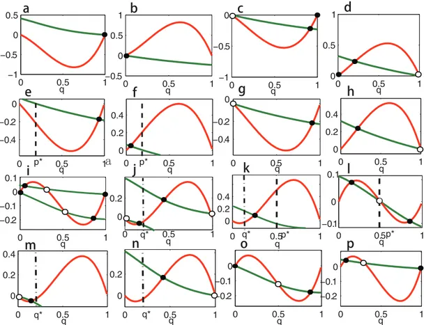
Fig 2. Solutions ofEq (7)and their stabilities under dynamics (2) whenc1>0 andc2= 0.Intersections ofh1(q) andh2(q) (i.e., the solutions ofEq (7)) are

shown for all sixteen possible situations. The red curves denoteh1(q) and the green curvesh2(q). The intersections denoted by black spots correspond to

stable equilibria of dynamics (2), and the intersections denoted by black circles correspond to unstable equilibria. Parameters are taken asβ1=β2= 0.01,α1

= 1,α2= 2 andc1= 0.5 in all sixteen panels. Payoff matrixes in the panels are: In panela,A= [1.5, 1.5; 0, 0],B= [5, 1; 0, 0]. In panelb,A= [0, 0; 1, 1],B= [0,

0; 5, 1]. In panelc,A= [1, 0; 0, 1],B= [3, 1; 0, 0]. In paneld,A= [1, 0; 0, 1],B= [0, 0; 3, 1]. In panele,A= [0, 1.25; 5, 0],B= [3, 1; 0, 0]. In panelf,A= [0, 1.25; 5, 0],B= [0, 0; 3, 1]. In panelg,A= [0, 0; 1, 1],B= [3, 1; 0, 0]. In panelh,A= [1, 1; 0, 0],B= [0, 0; 3, 1]. In paneli,A= [1, 0; 0, 1],B= [2, 0; 0, 1]. In panelj,A= [1, 0; 0, 1],B= [0, 1; 4, 0]. In panelk,A= [0, 2; 2, 0],B= [0, 1; 5, 0]. In panell,A= [0, 2; 2, 0],B= [1, 0; 0, 1]. In panelm,A= [0, 0; 1, 1],B= [0, 1; 4, 0]. In panel n,A= [1.5, 1.5; 0, 0],B= [0, 1; 4, 0]. In panelo,A= [0, 0; 1, 1],B= [2, 0; 0, 1]. In panelp,A= [1, 1; 0, 0],B= [2, 0; 0, 1]. The positions of the interior ESSsp* andq*(0<p*,q*<1) are marked by dashed lines.

doi:10.1371/journal.pone.0142929.g002

7. Ifp_{is an ESS forAandqis an ESS forB, then both the symmetric boundary equilibria}

ð0_;0_;^_n1;^_n2Þandð1_;1_;^_n1;^_{n2Þare unstable. Furthermore,Eq (7)has a unique (interior)} solution^_{q, which corresponds to an asymptotically stable equilibriumðp;}^_q;^_n1;^n2Þof dynamics (2). Similarly as (3), this equilibrium is also globally stable and two phenotypes will stably coexist in the system (seeFig 2K).

8. Ifpis an ESS forAand bothR1andR2are ESSs forB, then both the symmetric boundary equilibriað0_;0_;^_n1;^n2Þandð1;1;^n1;^n2Þare unstable. Furthermore,Eq (7)has at most three (interior) solutions, which are denoted by^_q1,^_q2andq^_3with^_q1<^_q2<^_{q3. The two} inte-rior equilibria corresponding to^_q1andq^3are stable under dynamics (2) and the interior equilibrium corresponding to^_{q2is unstable (seeFig 2L).}

9. IfR2(orR1) is the only ESS forAandq_{is an ESS forB, then both the symmetric boundary}

equilibriað0_;0_;^_n1;^_n2Þandð1_;1_;^_n1;^_{n2Þare unstable. Furthermore,Eq (7)has a unique} (interior) solution^_{q, which corresponds to an asymptotically stable equilibrium}

ð0_;^_q;^_n1;n^_2Þ(orð1_;^_q;^_n1;^_{n2Þ) of dynamics (2). Similarly as (4), this equilibrium is also} globally stable and two phenotypes will stably coexist in patch 2 (seeFig 2M and 2N).

10. IfR2(orR1) is the only ESS forAand bothR1andR2are ESSs forB, then the symmetric boundary equilibriumð0_;0_;^_n1;n^2Þ(orð1;1;n^1;^n2Þ) is stable and the otherð1;1;n^1;n^2Þ (orð0_;0_;^_n1;n^_{2Þ) is unstable. Furthermore,Eq (7)has at most two (interior) solutions,} where one corresponds to a stable equilibria of dynamics (2) and the other is unstable. Sim-ilarly as (2), either all individuals in the system displayR2(orR1), or individuals in patch 1 displayR2(orR1) and two phenotypes coexist in patch 2 (seeFig 2O and 2P).

Case 2.c1>0andc2>0. We now consider the case withc1>0 andc2>0. It is easy to check that dynamics (2) only have two boundary equilibria,ð0_;0_;n1^_;^_n2Þandð1_;1_;n1^_;n2^_{Þ, and} the existence of asymmetric boundary equilibrium is impossible, for instance, ifp= 0 andq6¼ 0, thendp

dt>0. We then focus on the number and stability of interior equilibria. Notice that an equilibrium of dynamics (2) should be the solution of equation

D1pð1 _{pÞðp pÞ þc2ðq pÞ}n2

n1 ¼ 0 ;

D2qð1 _{qÞðq qÞ þc1ðp qÞ}n1

n2 ¼ 0 ;

½

f þ ða1 b1n1Þ

Š

½

Š

ð8Þ

So if bothn1andn2are positive, then from thefirst two equations ofEq (8), an interior equilib-rium of dynamics (2) should obey the equations

D1D2pð1 pÞqð1 qÞðp p

_{Þðq qÞ ¼ c1c2ðp qÞ}2

: ð9Þ

Furthermore, from the third and the forth equations ofEq (8)

D1pð1 pÞðp p _Þ

c2ðp qÞ ¼

b1

b2

gþa2 c2þ D2qð1 qÞðq qÞ

q p

f þa1 c1þD1pð1 pÞðp pÞ

p q

where we assume that bothpandqare in the interval 0<p,q<1 (i.e., we consider the most complicated payoff structures).

FromEq (9), it is easy to see that for the situation withp6¼q, if the interior equilibrium exists, then it should be in the region (0,p_{) × (q, 1), or (p, 1) × (0,q) ifΔ}

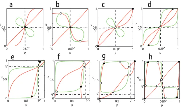
1Δ2>0, and in the region (0,p) × (0,q), or (p, 1) × (q, 1) ifΔ1Δ2<0. Of course, it is very difficult to get the exactly analytic solutions of Eqs (9) and (10) in general. The numerical analysis suggests that ten interior equilibria can exist (seeFig 3H). To show this, some examples are plotted inFig 3. All of these examples show clearly that the equilibrium structure of dynamics (2) could be very complicated.

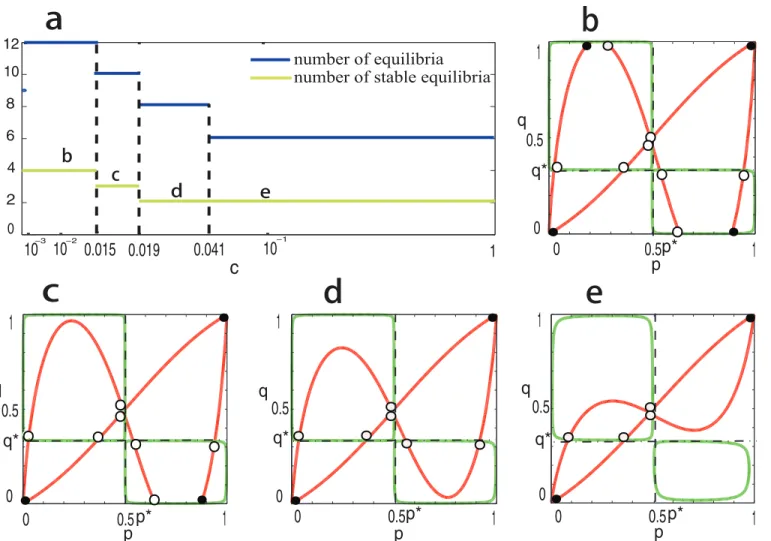
We further look at the bifurcation behaviors of system (2) for the case that bothR1andR2 are ESSs forAandB(i.e., the most complicated case), and assume equal migration rates between regions, i.e.,c1=c2=c. In this case, both the symmetric boundary equilibria ð0_;0_;n1^_;n2^_Þandð1_;1_;n1^_;^_{n2Þare asymptotically stable, and the system can have ten interior} equilibria. Whenc= 0, it is easy to see that the system has nine equilibria in total, including four stable (boundary) equilibria andfive unstable equilibria. The number of equilibria jumps from nine to twelve as soon as the migration rates becomes positive although the number of stable equilibria keeps unchanged (seeFig 4A and 4B). Furthermore, numerical simulation shows that both the numbers of stable equilibria and unstable equilibria decrease ascincreases. In particular, whenc>0.019, the system has only two stable equilibria (i.e., the two symmetric

Fig 3. Equilibria ofEq (2)on thep−qplane and their stabilities whenc1>0 andc2>0.The red curves correspond toEq (10)and the green curvesEq

(9). The intersections denoted by black spot correspond to stable equilibria of dynamics (2), and the intersections denoted by black circle correspond to unstable equilibria. Parameters are taken as: In panela,A= [0, 1; 1, 0],B= [0, 5; 5, 0],β1=β2= 0.01,α1= 1.25,α2= 1.8,c1= 0.25 andc2= 0.8. In panelb,A

= [0, 1; 1, 0],B= [0, 5; 5, 0],β1=β2= 0.01,α1= 1.125,α2= 0.1,c1= 0.125 andc2= 0.8. In panelc,A= [1, 0; 0, 1],B= [5, 0; 0, 5],β1=β2= 0.001,α1= 1.4,α2

= 1.5,c1= 0.4 andc2= 0.5. In paneld,A= [0, 1; 1, 0],B= [5, 0; 0, 5]β1=β2= 0.001,α1= 1.5,α2= 1.2,c1= 0.5 andc2= 0.2. In panele,A= [0, 5; 1, 0],B= [1,

0; 0, 5],β1=β2= 0.001,α1= 1.5,α2= 1.2,c1= 0.5 andc2= 0.2. In panelf,A= [0, 5; 1, 0],B= [0, 1; 5, 0],β1=β2= 0.001,α1= 1.5,α2= 1.2,c1= 0.5 andc2=

0.2. In panelg,A= [1, 0; 0, 5],B= [5, 0; 0, 1],β1=β2= 0.001,α1= 1.4,α2= 1.5,c1= 0.4 andc2= 0.5. In panelh,A= [1, 0; 0, 1],B= [2, 0; 0, 1],β1= 0.05,β2=

0.01,α1= 1.75,α2= 2,c1= 0.25 andc2= 0.01. The positions ofp*andq*are marked by dashed lines (0<p*,q*<1, and note thatp*andq*may not be

ESS).

doi:10.1371/journal.pone.0142929.g003

boundary equilibria), and all interior equilibria are unstable (seeFig 4). These results suggest that small migration rates make the dynamical behavior of the system more complex.

Discussion

A vast amount of research has been devoted to analyze the influence of spatial diffusion on the evolutionary stability of ecology systems. One well known mathematical approach is the reac-tion-diffusion equation, where in this framework, individuals are dispersed in a continues space [10–11,17–21]. For instance, Hofbauer et al. [11,21] considered a population of two types of individuals distributed in an one-dimensional space, and assumed that the migration (or diffusion) rate is both individual-independent and location-independent. They showed that in two-strategy coordination games, if the reaction term of the reaction-diffusion equation is taken as replicator dynamics, then one strategy will drive out the other strategy in form of a traveling wave front, although there is no simple rule to decide which strategy can survive.

Fig 4. Bifurcation behaviors ofEq (2)whenc1>0 andc2>0.In panela, the number of equilibria and the number of stable equilibria are denoted by blue

line and yellow line, respectively. In panelsb-e, the red curves correspond toEq (10)and the green curvesEq (9). The intersections denoted by black spot correspond to stable equilibria of dynamics (2), and the intersections denoted by black circle correspond to unstable equilibria. The positions ofp*andq*are marked by dashed lines. Parameters are taken as:A= [1, 0; 0, 1],B= [2, 0; 0, 1],β1= 0.05,β2= 0.01,α1= 1.75,α2= 2. In panelb,c1=c2=c= 0.014; in

panelc,c1=c2=c= 0.015; in paneld,c1=c2=c= 0.02; and in panele,c1=c2=c= 0.05.

In this paper, we assume that individuals are distributed in a (discrete) patchy environment. Following Prior et al. [6], we investigate a simple two-phenotype and two-patch model, where individuals compete only with their immediate neighbors and the migration rates between patches are individual-independent but patch-dependent. Different from Prior et al. [6] who focused on the homogeneous patchy environment, we here are more interested in the dynam-ical stability in heterogeneous environment. Our main results show that: (i) if the pure strategy R1(orR2) is an ESS for both two patches, then the boundary equilibrium corresponding to p= 1 andq= 1 (orp= 0 andq= 0) must be asymptotically stable; (ii) if the payoff matricesA

andBsatisfyp _¼ a12 a22

a12 a22þa21 a11¼q

_¼ b12 b22

b12 b22þb21 b112 ð

0_;1_{Þ, then the interior equilibrium}

cor-responding to (p_{,q) is asymptotically stable ifpis an ESS forAandqan ESS forB; (iii) as a} special case withc1>0 andc2= 0 (orc1= 0 andc2>0), i.e. individuals can only move from patch 1 to patch 2 (or from patch 2 to patch 1), all possible situations for the existence and sta-bility of boundary and interior equilibria are considered, and wefind that dynamics (2) can have six equilibria where four of them are stable; (iv) forc1>0 andc2>0, the numerical analy-sis shows that the equilibrium structure and dynamical behavior of the system could be very complicated in general. In particular, dynamics (2) can have twelve equilibria where four of them are stable.

Our analysis provides an insight for understanding the effect of spatial dispersion on the evolutionary stability of patchy environment. Both the analytical analysis and the numerical simulation indicate that the original ESS formulations which ignore the dispersion process can-not be applied to predict the evolutionary outcome of the dispersion system even for small migration rates. For instance, in the case that both patches have multiple ESS’s and no dispersal between patches, the system has four (boundary) stable equilibria and five unstable equilibria. However, if one ofc1andc2becomes positive, the system can have two to four stable equilibria and four to eight unstable equilibria. Furthermore, we found that both the numbers of stable equilibria and unstable equilibria decrease in the migration rates. This observation has an intui-tive biological interpretation [6]. In a heterogenous patchy environment, the effect of selection is to make the overall population more heterogeneous in the sense of different patches have dif-ferent population compositions, while the effect of migration is to move the population compo-sition in each patch towards the mean of the overall population, i.e., migration promotes homogeneity. Thus, when the migration rates are small (i.e., the effect of selection is strong), similarly as the case of no dispersal, the system has two stable symmetric boundary equilibria and two stable asymmetric equilibria; and when the migration rates are large (i.e., the effect of migration is strong), the existence of stable asymmetric equilibrium is impossible, and the sys-tem has only two stable symmetric boundary equilibria, where at these equilibria all individuals display the same phenotype.

In this paper, we focus on the effect of spatial dispersion on two-patch system only. A natu-ral extension would be to consider the three-patch system. However, analyzing the dynamical behavior of the three-patch system may be an even more difficult issue because the equilibrium structure of the two-patch system is already very complex. Another possible development would be to compare the evolutionary stability of the patchy environment under different migration rules. One commonly used migration rule is that individuals know perfectly the pay-off in all patches and they always move to the patch with the highest paypay-off (i.e., ideal animals) [15]. In contrast, a more realistic model is that individuals do not migrate to patches with lower payoff [22]. Recent studies have shown that these two migration rules can lead to the IFD [16,23]. Since that the IFD corresponds to a stable equilibrium of the non-dispersed evo-lutionary dynamics, we can then expect that these migration rules may also lead to the ESS of the non-dispersed evolutionary dynamics [23].

Methods

Stability of the symmetric equilibria

The Jacobian matrix of the dynamics (2) about the symmetric boundary equilibrium ð1_;1_;n1^_;n2^_{Þ, denoted byJ}

(1,1), is

ða11 a21Þ c2_n^2

^

n1 c2

^ n2

^ n1

0 0

c1_n^1

^

n2 ðb11 b21Þ c1

^ n1

^ n2

0 0

ð2_{a11 a12 a21Þn1}^ 0 _b1n1^ _c2n^2

^

n1 c2

0 _ð2_{b11 b12 b21Þn2}^ _{c1 b2n2}^ _c1^n1

^ n2 0 B B B B B B B B B @ 1 C C C C C C C C C A ;

and similarly, the Jacobian matrix aboutð0_;0_;n1^_;^_{n2Þ, denoted byJ(0,0), is}

ða12 a22Þ c2_n^2

^

n1 c2

^ n2

^ n1

0 0

c1_n^1

^

n2 ðb12 b22Þ c1

^ n1

^ n2

0 0

ða12þa21 2_a22Þn1^ 0 _b1n1^ _c2n^2

^

n1 c2

0 _ðb12þb21 2_b22Þn2^ _{c1 b2n2}^ _c1^n1

^ n2 0 B B B B B B B B B @ 1 C C C C C C C C C A :

For the matrixJ_(1,1), notice that the eigenvalues of the matrix

ða11 a21Þ c2^n2

^

n1 c2

^ n2

^ n1

c1^_n1

^

n2 ðb11 b21Þ c1

^ n1 ^ n2 0 @ 1 A

have negative real parts ifa11−a21>0 andb11−b21>0, and that the real parts of the eigen-values of the matrix

b1_n1^ _c2n^2

^

n1 c2

c1 b2^_{n2 c1}n^1

^ n2 0 @ 1 A

must be negative. So, if the pure strategyR1is an ESS for both payoff matricesAandB, then the eigenvalues ofJ_(1,1)must have negative real parts [6]. Similar to the matrixJ_(0,0), if the pure strategyR2is an ESS for both payoff matricesAandB, then the eigenvalues ofJ_(0,0)have nega-tive real parts.

The Jacobian matrix about the symmetric interior equilibriumðp_;q;n1^_;^_{n2Þ, denoted by}

J_(p,q), is

p_{ð1 pÞ}

D1 c2 ^ n2

^

n1 c2

^ n2

^ n1

0 0

c1^n1

^

n2 q

_{ð1 qÞ}

D2 c1 ^ n1

^ n2

0 0

ð a12þa21Þ_n1^ 0 _b1n1^ _c2^n2

^

n1 c2

0 _{ð b12þb21Þn2}^ _{c1 b2}^_{n2 c1}n^1

^ n2 0 B B B B B B B B B @ 1 C C C C C C C C C A ;

(or the matrixJ_(0,0)), the eigenvalues ofJ_{(p,q)have the negative real parts ifp(=q) is an} ESS for both payoff matricesAandB, i.e., the equilibriumðp_{;q;^n1;n2^Þis asymptotically} sta-ble ifp_{(=q) is an ESS for bothAandB.}

Stability analysis of dynamics (6) when

c

>

0 and

c

= 0

We first analyze the solutions ofEq (7). For convenience, let

h1ðqÞ ¼ D2qð1 _{qÞðq qÞ;}

h2ðqÞ ¼

^

p q

2

ffiffiffiffiffiffiffiffiffiffiffiffiffiffiffiffiffiffiffiffiffiffiffiffiffiffiffiffiffiffiffiffiffiffiffiffiffiffiffi

ða2þ_gÞ2_þ4_b2c1n1^ q

ða2þ_gÞ

:

It is easy to see thatEq (7)has a boundary solution^_q¼0_{(orq= 1) if and only if}^_p¼0_(or ^

p¼1_{). Furthermore, the interior solutions ofEq (7)should correspond to the intersections of} the functionsh1(q) andh2(q) in the interval 0<q<1. Notice thath1(0) =h1(1) =h1(q) = 0, Δ2h1(q)>0 for 0<q<qandΔ2h1(q)<0 forq<q<1 (if 0<q<1), and thath2(0)0, h2(1)0,h2ð^_{pÞ ¼}0_{,h2(q)>0 for}0_<q<p^_{andh2(q)<0 forp}^_<q<1_(if0_<^_p<1_). Then, for the existence of intersections in the interval 0<q<1, we have that:

1. IfR1is the only ESS for both payoff matricesAandB, then, no intersection can exist (see

Fig 2A); and, similarly, ifR2is the only ESS for bothAandB, then no intersection can exist (seeFig 2B).

2. If bothR1andR2are ESSs forAbutR1is the only ESS forB, then only one intersection exists (seeFig 2C); and, similarly, if bothR1andR2are ESSs forAbutR2is the only ESS for

B, then only one intersection exists (seeFig 2D).

3. Ifp2(0, 1) is an ESS forAandR1is the only ESS forB, only one intersection exists (see

Fig 2E); and, similarly, ifpis an ESS forAandR2is the only ESS forB, then only one inter-section exists (Fig 2F).

4. IfR2is the only ESS forAandR1is the only ESS forB, then only one intersection exists (see

Fig 2G); and, similarly, ifR1is the only ESS forAandR2is the only ESS forB, then only one intersection exists (seeFig 2H).

5. If bothR1andR2are ESSs forAandB, then at most four intersections can exist (seeFig 2I).

6. If bothR1andR2are ESSs forAandq2(0, 1) is an ESS forB, only two intersections exist (seeFig 2J).

7. Ifpis an ESS forAandqis an ESS forB, the only one intersection exists (seeFig 2K).

8. Ifpis an ESS forAand bothR1andR2are ESSs forB, then there are at most three intersec-tions (seeFig 2L).

9. IfR2is the only ESS forAandqis an ESS forB, then only one intersection exists (seeFig 2M); and, similarly, IfR1is the only ESS forAandqis an ESS forB, then only one intersec-tion exists (seeFig 2N).

10. IfR2is the only ESS forAand bothR1andR2are ESSs forB, then there are at most two intersections (seeFig 2O); and, similarly, ifR1is the only ESS forAand bothR1andR2are ESSs, then there are at most two intersections (seeFig 2P).

For the stability of the solutions ofEq (7)under dynamics (6), it is easy to see that for given ^

p(i.e._p^_{2 f}0_;1_{;pgcorresponds to the stable equilibrium of dynamics (5)), if~q¼}^_pand~_qis an ESS for the payoff matrixB, then the corresponding equilibriumð~_q;^_{n2Þmust be}

asymptotically stable under dynamics (6). On the hand, letð^_q;^_{n2Þbe an interior equilibrium of} dynamics (6), and the Jacobian matrix aboutð^_q;^_{n2Þ, denoted by}J_ð^

q;_n^2Þ, is given by

J_ð^q

;n^2Þ ¼

h1ðqÞ

dq jq¼_q^ c1 ^

n1 ^

n2

ð^_p ^_qÞc1^n1

^ n2

2

d_gðqÞ

dq jq¼_q^n2^ c1 ^ n1

^ n2 b2

^ n2 0 B B B B @ 1 C C C C A :

Clearly, the interior equilibriumð^_q;n2^_{Þis asymptotically stable (i.e. the eigenvalues of}J_ð^

q;_n^2Þ

have the negative real parts) if

h1ðqÞ

dq jq¼^_q 2c1 ^ n1 ^

n2 b2^n2 < 0 ; h1ðqÞ

dq jq¼^_qþc1 ^ n1 ^ n2

c1n^1

^ n2þb2

^

n2þ ð^_p ^_qÞc1n1^ ^ n2

d_gðqÞ

dq jq¼^_q > 0 :

Thus, for given parameter values, stabilities of the interior equilibria of dynamics (6) (i.e., interior solutions ofEq (7)) can be analyzed numerically according to the above conditions (see the figure caption ofFig 2for detailed parameters, note that the following results may not be true for all parameter values).

1. IfR1(orR2) is the only ESS forAandB, then the boundary equilibriumð1_;^_n2Þwith^p¼1 (orð0_;n^_2Þwith^_p¼0_{) is asymptotically stable (see alsoFig 2A and 2B).}

2. If bothR1andR2are ESSs forAbutR1(orR2) is the only ESS forB, then one boundary equilibriumð0_;n^_2Þwith^_p¼0_(orð1_;^_n2Þwithp^_¼1_{) is unstable and the other boundary} equilibriumð1_;n^2Þwith^p¼1(orð0;n^2Þwith^p¼0) is asymptotically stable. Furthermore, the unique interior equilibriumð^_q;^_{n2Þis also asymptotically stable (see alsoFig 2C and}

2D).

3. Ifpis an ESS forAandR1(orR2) is the only ESS forB, then the unique interior equilib-rium is asymptotically stable (see alsoFig 2E and 2F).

4. IfR2(orR1) is the only ESS forAbutR1(orR2) is the only ESS forB, then the boundary equilibriumð0_;n^2Þwith^p¼0(orð1;^n2Þwithp^¼1) is unstable and the unique interior equilibrium is asymptotically stable (see alsoFig 2G and 2H).

5. If bothR1andR2are ESSs forAandB, then the boundary equilibriumð1_;n^2Þwith^p¼1, or the boundary equilibriumð0_;^_n2Þwith^_p¼0_{, is stable, and for four interior equilibria,} two are stable and the other two are unstable (see alsoFig 2I).

6. If bothR1andR2are ESSs forAandqis an ESS forB, then the boundary equilibrium ð1_;^_n2Þwith^p¼1, or the boundary equilibriumð0;^n2Þwithp^¼0, is unstable, and the two interior equilibria are asymptotically stable (see alsoFig 2J).

7. Ifp_{is an ESS forAandqis an ESS forB, then the unique interior equilibrium is}

asymptot-ically stable (see alsoFig 2K).

8. Ifp_{is an ESS forAand bothR1andR2are ESSs forB, then there are at most three interior}

equilibria corresponding to three intersections ofh1andh2, which are denoted by^_q1,q^_2and ^

9. IfR2(orR1) is the only ESS forAandq_{is an ESS forB, then the boundary equilibrium}

ð0_;^_n2Þwith^_p¼0_(orð1_;n^_2Þwith^_p¼1_{Þis unstable and the unique interior equilibrium is} asymptotically stable (see alsoFig 2M and 2N).

10. IfR2(orR1) is the only ESS forAand bothR1andR2are ESSs forB, then there are at most two interior equilibria, the boundary equilibriumð0_;^_n2Þfor^p¼0(orð1;^n2Þfor^p¼1) is stable, and one interior equilibrium is stable and the other unstable (see alsoFig 2O and 2P).

Author Contributions

Conceived and designed the experiments: QL JZ BZ RC YT. Performed the experiments: QL JZ BZ RC YT. Analyzed the data: QL JZ BZ RC YT. Contributed reagents/materials/analysis tools: QL JZ BZ RC YT. Wrote the paper: QL JZ BZ RC YT.

References

1. Maynard Smith J, Price GR. The logical animal conflict. Nature. 1973; 246: 15–18. doi:10.1038/ 246015a0

2. Taylor PD, Jonker LB. Evolutionarily stable strategies and game dynamics. Math. Biosci. 1978; 40: 145–156. doi:10.1016/0025-5564(78)90077-9

3. Maynard Smith J. Evolution and the Theory of Games. Cambridge University Press; 1982.

4. Cressman R. The stability concept of evolutionary game theory: a dynamic approach. Lect Notes Bio-math. vol. 94, Berlin, Heildelberg New York: Springer; 1992.

5. Hofbauer J, Sigmund K. Evolutionary Games and Population Dynamics. Cambridege University Press; 1998.

6. Prior TG, Hines WGS, Cressman R. Evolutionary games for spatially dispersed populations. J. Math. Biol. 1993; 32: 55–65.

7. Ludwig D, Levin SA. Evolutionary stability of plant communities and the maintenance of multiple dis-persal types. Theor. Popul. Biol. 1991; 40: 285–307. doi:10.1016/0040-5809(91)90057-M

8. Comins HN, Hamilton WD, May RM. Evolutionary stable dispersal strategies. J. Theor. Biol. 1980; 82: 205–230.

9. Levin SA, Cohen D, Hastings A. Dispersal strategies in patchy environments. Theor. Popul. Biol. 1984; 26: 165–191. doi:10.1016/0040-5809(84)90028-5

10. Hutson VCL, Vickers GT. Traveling waves and dominance of ESS’s. J. Math. Biol, 1993; 30: 457–471.

doi:10.1007/BF00160531

11. Hofbauer J, Hutson VCL, Vickers GT. Travelling waves for games in economics and biology. Nonlinear. Anal. Theor. 1997; 30:1235–1244. doi:10.1016/S0362-546X(96)00336-7

12. Dieckmann U, O’Hara B, Weisser W. The evolutionary ecology of dispersal. Trends Ecol. Evol. 1999; 14: 88–90. doi:10.1016/S0169-5347(98)01571-7

13. Travis JMJ, Murrell DJ, Dytham C. The evolution of density dependent dispersal. Proc. R. Soc. Lond. B. 1999; 266: 1837–1842. doi:10.1098/rspb.1999.0854

14. Hines WGS, Maynard Smith J. Games between relatives. J. Theor. Biol. 1979; 79: 19–30. doi:10.

1016/0022-5193(79)90254-6PMID:513800

15. Fretwell SD, Lucas HL. On Terriotorial behavior and other factors influcing habitat distribution in birds. Acta Bio-theoretica. 1970; 19: 16–32. doi:10.1007/BF01601953

16. Cressman R, Krivan V. Migration dynamics for the ideal free distribution. Am. Nat. 2006; 168: 384–

397. doi:10.1086/506970PMID:16947113

17. Sun GQ, Jin Z, Li L, Haque M, Li BL. Spatial patterns of a predator-prey model with cross diffusion. Non-linear. Dynam. 2012; 69: 1631–1638.

18. Sun GQ, Zhang J, Song LP, Jin Z, Li BL. Pattern formation of a spatial predator-prey system. Appl. Math. Comput. 2012; 218: 11151–11162. doi:10.1016/j.amc.2012.04.071

19. Sun GQ, Chakraborty A, Liu QX, Jin Z, Anderson KE, Li BL. Influence of time delay and nonlinear diffu-sion on herbivore outbreak. Commun. Nonlinear. Sci. 2014; 19: 1507–1518. doi:10.1016/j.cnsns. 2013.09.016

20. Sun GQ, Wang SL, Ren Q, Jin Z, Wu YP. Effects of time delay and space on herbivore dynamics: link-ing inducible defenses of plants to herbivore outbreak. Sci. Rep. 2015; 5: 11246. doi:10.1038/

srep11246PMID:26084812

21. Hofbauer J. The spatially dominant equilibrium of a game. Ann. Oper. Res. 1999; 89: 233–251. doi:10. 1023/A:1018979708014

22. Hugie DM, Grand TC. Movement between patches, unequal competitors and the ideal free distribution. Evol. Ecol. 1998; 12: 1–19.