Parametrization of the precipitation in the Northern Hemisphere and its verification in Mexico

Parametrization of the precipitation in the Northern Hemisphere

and its veri®cation in Mexico

V. M. Mendoza, B. Oda, J. Adem

Centro de Ciencias de la AtmoÂsfera, Universidad Nacional AutoÂnoma de MeÂxico, 04510, MeÂxico D. F., MeÂxico

Received: 5 February 1997 / Revised: 15 December 1997 / Accepted: 17 December 1997

Abstract. To improve results in monthly rainfall pre-diction, a parametrization of precipitation has been developed. The thermodynamic energy equation used in the Adem thermodynamic model (ATM) and the Clausius and Clapeyron equation, were used to obtain a linear parametrization of the precipitation anomalies as a function of the surface temperature and the 700 mb temperature anomalies. The observed rainfall in Mexico over 36 months, from January 1981 to December 1983, was compared with the results obtained of the heat released by condensation, which is proportional to precipitation, using our theoretical formula, and those obtained using a statistical formula, which was derived for the ATM using 12 years of hemispheric real data. The veri®cation using our formula in Mexico, showed better results than the one using the statistical formula.

Key words. Meteorology and atmospheric dynamics (climatology; convective processes; general circulation).

1 Introduction

The objective of this work is to obtain a parametrization of the precipitation anomalies, as a linear function of the surface temperature and the 700 mb temperature anom-alies, in order to improve the prediction in monthly precipitation, using the Adem thermodynamic model (ATM).

The statistical parametrization of the precipitation which has been used in the ATM for the prediction of monthly precipitation in the United States (Adem and Donn, 1981), and in Mexico (Ademet al., 1995), and in climate simulations (Adem, 1996), was derived by Clapp

et al. (1965), as a multiple regression equation for

precipitation. They assumed that the anomaly of the total monthly precipitation can be expressed as a simple linear function of the local anomalies of mean-monthly temperature and the west-east and the south-north wind components at 700 mb. These three variables were chosen simply because there are physical reasons for expecting them to be related to precipitation. They assume the following linear regression equation

RÿRN ˆb T7… ÿT7N† ‡c U7… ÿU7N† ‡d V7… ÿV7N† …1†

where R is the total monthly precipitation (inches); T7

the monthly mean temperature … †K at 700 mb, andU7

and V7, the horizontal wind components …m sÿ1† at 700 mb, regarded as positive when from west to east and from south to north, respectively. The subscriptN refers to normal or long period averages which, in this study, were the sample means. In order to determine the regression coecients,b;candd, approximately 12 y of monthly-mean data for 37 land or island stations scattered over the Northern Hemisphere were used. Data for individual stations were extracted from a variety of sources. In the vast areas where there were no measured precipitation ®gures (mainly over oceans) or where no computations were made, certain reasonable guidelines were followed based on the available calcu-lations and on synoptic experience.

In spite of inadequate data coverage and low correlations, it was concluded that the geographical pattern of the temperature coecient …b†, depends mainly on climate.

The distribution of the wind component coecients,

candd, was assumed to depend mainly on terrain and latitude. Where westerly or southerly wind is directed from water to land and especially if it is forced to ascend mountains, a strong positive relationship between rain-fall and wind is found, (demonstrated in Negri et al., 1993). When it is directed downslope, these components are negatively related to rainfall. The south-north wind component,V, tends to be positively related to rainfall almost everywhere due to the observed fact that convergence and rising motion prevails with southerly winds and the opposite with northerly wind.

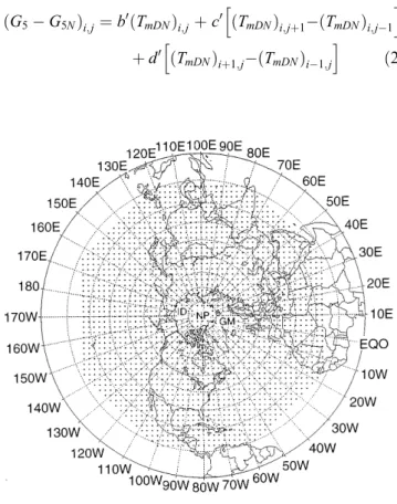
Equation (1) had to be modi®ed in order to be used in the ATM because the latter predicts the mean temper-ature in mid-troposphere (approximately 500 mb) and not the winds. The mid-tropospheric temperature anomalies can be used directly in the ®rst term on the right of Eq. (1), assuming there is little di€erence in the anomaly of monthly mean temperature at 500 and 700 mb. However, the two terms involving the winds must be transformed in two important respects. First, the predictions are made for the NMC grid, which is a grid array of 1977 points on a polar-stereographic projection over the Northern Hemisphere, whoseX axis points along the 10_{E meridian and Y axis along the} 80_{W meridian (Fig. 1). Therefore, it is necessary to} transform the eastward …U† and northward …V† wind components to the corresponding components U0 and

V0, directed along the positiveX andY axes respectively by a simple transformation of coordinates. The second transformation is to convert the wind into a thermal wind (a measure of vertical wind shear), so that the wind components at 700 mb can be replaced by temperature gradients in mid-troposphere. The details of these transformations are not documented here.

Finally, the rainfall (R) in inches per month may be expressed in terms of the heat released by conden-sation …G5† in the atmosphere …cal cmÿ2 dayÿ1

0:484 W mÿ2_{†, by multiplying R in cm day}ÿ1 _{by the}

latent heat of condensation …L† in cal gÿ1 _{and by the}

water density q_w in g cmÿ3_.

Using these transformations, Eq (1) becomes:

G5ÿG5N

… †_i;jˆb0…TmDN†i;j‡c0 …TmDN†i;j‡1ÿ…TmDN†i;jÿ1

h i

‡d0 …TmDN†i‡1;jÿ…TmDN†iÿ1;j

h i

…2†

where …G5ÿG5N† is expressed in cal cmÿ2 _dayÿ1

; the subscripts i andj, are index numbers identifying the X

and Y coordinates, respectively, of the NMC grid. DN

denotes the departure from normal of mid-tropospheric temperature,…TmÿTmN†inK; and the wind components

are replaced by temperature gradients in the mid-troposphere. Finally, the transformed coecients b0, c0

and d0 were determined as functions of the statistical regression coecients b, c and d interpolated at each grid point.

2 Theoretical parametrization

For the parametrization of precipitation we will try to develop a theoretical linear formula similar to Eq. (2), to be used in the ATM and attempt to improve the results in monthly rainfall prediction.

We start with the thermodynamic energy equation which can be expressed as

qcpdT

dt ÿ

dP dt ˆQ

R

‡Q_s

‡Q_T

ÿLqdq

s

dt ‡Q

cc

…3†

where cp is the speci®c heat at constant pressure of the

humid air;T,Pandqare the three-dimensional ®elds of temperature, pressure and density;Q_R is the heating rate due to long and shortwave radiation; Q_s is the heating rate of sensible heat given o€ to the atmosphere by vertical turbulent transport and Q_T is the heating rate due to the divergence of horizontal turbulent ¯ux of heat. The total heat released by condensation is of two forms (Washington and Williamson, 1977):

ÿLq_dq

s=dt, referred to as stable latent heat release,

where Lis the latent heat of vaporization and q_s is the saturated speci®c humidity.Q_cc, is the heat released by precipitation associated with convection cumulus activ-ity which usually dominates over the equator, the tropics and higher latitude continental areas in the summer.

The three-dimensional ®eld of temperature in the atmosphere is expressed by:

TˆT‡b…Hÿz† …4†

where b is the constant lapse rate of the standard atmosphere and T is the temperature of zˆH, where

H ˆ9 km is the height of the ATM.

Using Eq. (4) together with the hydrostatic equilib-rium and the perfect gas equations we obtain:

P ˆP T

T a

…5†

q ˆq T

T aÿ1

…6†

whereP andqare the corresponding values ofPandq

at zˆH, and aˆg=Rb; g is the gravitational acceler-ation; andR is the gas constant of humid air.

The saturated speci®c humidity is given with good degree of approximation by:

Fig. 1. NMC grid used in the Adem thermodynamic model: 1977

points distributed in a polar stereographic projection whereX andY

coordinate axes were arbitrarily determinated along 10_{E and 80W,}

q_s ˆ0:622e

s

P …7†

wheree_s is the saturation water vapor pressure, which is a function of temperature and can be expressed with a simple formula (Adem, 1967a):

e_s ˆa1‡b1t‡c1t2‡d1t3‡l1t4 …8†

where e_s is in millibars and tˆTÿ273:16_{C; T is} the absolute temperature given by Eq. (4); a1ˆ6:115,

b1ˆ0:42915, c1ˆ0:014206, d1ˆ3:04610ÿ4 _and l1ˆ3:210ÿ6_.

The relative change of the saturation vapor pressure is related to the relative change of temperature by the Clausius ± Clapeyron equation:

de s e s ˆ L Rv dT

T2 …9†

where Rv is the gas constant of water vapor. Using Eqs. (7) and (9) we obtain:

1

q

s

dq_s

dt ˆ L RvT2

dT

dt ÿ

1

P dP

dt …10†

By introducing dT=dt from Eq. (3), into Eq. (10), we obtain:

Lqdq

s

dt ˆ Lq_s

P

LP_ÿqc

pRvT2 L2_q

s‡cpRvT2

dP

dt

‡

L2q_s Q_R‡Q_s‡Q_T‡Q_cc

L2_q

s‡cpRvT2

…11†

Using the perfect gas equation and the approximation dP=dt ÿqgW where W denotes the vertical component of wind, we obtain the stable latent heat release:

ÿLqdq

s

dt ˆ Lqgq_s

R

LRÿcpRvT L2_q

s‡cpRvT2

Wd

ÿ L2_q

s QR

‡Q_s‡Q_T ‡Q_cc

L2_q

s‡cpRvT2

d0 …12†

where

dˆ 1:if W

_{>0 andqq}

s

0:if W0 or q<q_s

…13†

d0ˆ 1:ifq

_q

s

0:ifq<q_s

…14†

and where q is the speci®c humidity, which can be computed from the conservation of water vapor equa-tion. In Eq. (12), the ®rst term of the right hand side represents the latent heat release by adiabatic ascent of saturated air when dˆ1; and the second term repre-sents the latent heat release by non-adiabatic cooling of saturated air whend0ˆ1.

We assume that all water vapor is concentrated below the 500 mb surface; therefore the total heat released by condensation of water vapor G5, for a

vertical column ofH1height at 500 mb and unit area, is obtained integrating the following equation from the surface inzˆhto zˆH1:

G5ˆ ÿ ZH1

h

Lqdq

s

dt dz‡ ZH1

h Q_cc

dz …15†

wherehis the height of the terrain. Substituting Eq. (12) into Eq. (15) we obtain:

G5ˆgL R

ZH1

h

dqq_s LRÿcpRvT

L2_q

s‡cpRvT2

Wdz

ÿL2 ZH1

h

d0q_s Q

R

‡Q_s‡Q_T‡Q_cc L2_q

s‡cpRvT2 0

@

1

Adz‡ ZH1

h

Q_cc dz

…16†

A diagnostic formula for the vertical wind,W, has been derived by Adem (1967b), showing that the use of the divergence of geostrophic wind is a good working method for the computations of vertical wind when dealing with average states over periods of a month. In this work, we use Adem's formula for W, with some subsequent modi®cations carried out by Mendoza (1992), obtaining

W ˆqa

qWE‡ g

1ÿ

q_a qg1

J…f;P† ‡ g₂ÿqa

qg2

J…f;T†

…17†

where

g₁ ˆ RT

2

f2_{Pb a… ‡1†}

and

g₂ ˆ gT

f2_Tb2 T

aÿ

T

a‡1

where

aˆ g

Rb andgjˆ g

j

zˆh with jˆ1;2

q_a ˆq Ta

T aÿ1

…18†

Taˆb…Hÿh† ‡T …19†

q_aandTagiven by Eqs. (18) and (19) are the density and

the temperature at zˆh, respectively. In Eq. (17), the terms of the JacobiansJ…f;P†andJ…f;T†correspond to the divergence of geostrophic wind and WEˆ …W†zˆh

given by

WEWa‡ 1

q_a f bk r sa

…20†

induced by the terrain slope, which plays a key role in de®ning the local main rain features (Negriet al., 1993) and sa is the surface stress.Wa is given by

Wa ˆ!Va rh …21†

where !Va is the horizontal surface wind. The

compo-nent along theZ axis (pointing toward the local zenith) of the rotational of surface stress, can be approximated by

b

k r sa ˆqaCD V ! aN @_@va

x ÿ

@ua

@y

…22†

where CDˆ1:510ÿ3 is the drag coecient of the

wind, (Kasahara and Washington, 1967). j!VaNj is the

normal value of the horizontal surface wind speed taken from ATM climatological ®les;ua andva are theX and Y components of the horizontal surface wind, respec-tively, where the directions of the horizontal coordinates axes are arbitrarily chosen.

In Eqs. (21) and (22), !Va is assumed to be a

geostrophic wind. Therefore, in order to obtain its components we use the three-dimensional geostrophic wind for a layer of heightH with a constant lapse rate, obtaining:

uˆ ÿR f

T

T ‡a 1ÿ T

T

@T

@y ÿ RT

fq

@q

@y …23† vˆR

f T

T ‡a 1ÿ T

T

@T

@xÿ RT

fq

@q

@x …24†

According to Adem (1967b), the contribution of the terms containing@q=@xand@q=@yin formulas (23) and (24) is negligibly small compared with the terms containing @T=@x and @T=@y. Therefore, evaluating the componentsu and v forzˆh, we obtain

uaˆ ÿRs f

@T

@y …25†

vaˆRs f

@T

@x …26†

where

RsˆR Ta

T ‡a 1ÿ Ta

T

…27†

Substituting Eqs. (25) and (26) into Eqs. (21) and (22), and the resulting expressions in Eq. (20), we obtain:

WEˆ ÿ Rs

f J…h;T† ‡

CD!VaN f2 Rsr

2_{T …28†}

Using the approximation J…f;P† qRJ…f;T† ˆ …P=T†J…f;T†, and Eq. (28) into Eq. (17), we obtain:

Wˆ ÿqa

q

Rs f J…h;T†

‡ P

T g

1ÿ

q_a qg1

‡ g₂ÿqa

qg2

…f;T† …29†

3 The heating rates

The heating rate due to radiation,Q_R, is given by Adem, (1968b) as

Q_R

ˆET

H …30†

whereET is the excess of radiation in the layer of depth

H and is parametrized by the formula (Adem, 1964):

ET ˆF30‡F₃₀0 e‡F31T0‡ F32‡F₃₂0 eN

ÿ

T_s0‡…a2‡b3e†I …31†

whereF30,F300 ,F31,F32andF320 are constants;a2 andb3,

are climatological functions of latitude and season, obtained in Adem, (1964);I is the mean monthly solar radiation, which is computed from Milankovich formu-la; T0ˆTÿT0 and T_s0ˆTsÿTs0 are the departures from T (the mean temperature at zˆH), and Ts (the

mean surface temperature), andT0T0, andT_s0Ts0,

respectively, where T0 ˆ229:5 K and Ts0ˆ288 K are constants; e is the fractional cloud cover and eN is the

corresponding normal value (taken from ATM clima-tological ®les).

The fractional cloud cover is given by (Clappet al., 1965):

eˆeN‡d2…G5ÿG5N† …32†

whered2ˆ6:95910ÿ3_Wÿ1_{s is the empirical constant}

between the anomalies of cloudiness and the heat released by condensation of water vapor,G5:

The heating rate of sensible heating added to the atmosphere by vertical turbulent transport,Q_s, is given by Adem (1968b), as

Q_s

ˆG2

H …33†

where G2 is the sensible heating given o€ to the atmospheric layer of depth H, by vertical turbulent transport which was parametrized by Clapp et al., (1965) and is expressed as

G2ˆG2N ‡ V ! aN

G00₂K2‡ 1ÿG002

ÿ

K3

T_s0ÿT_sN0

ÿ

ÿ…T0ÿTN†

…34†

where

G00₂ ˆ 1; for oceans

0; for continents

K2andK3are constant parameters andG2N,T_sN0 andT_N0

are the normal values of G2, T_s0 and T0, respectively (Adem, 1965).

The heating rate due to the divergence of horizontal turbulent ¯ux, can be written by (Mendoza, 1992):

Q_T

ˆcpqK_r2_{T …35†}

where cp is the speci®c heat at constant pressure, q is given by Eq. (6), and T by Eq. (4); and K is the Austausch coecient.

cumulus activity was parametrized by Kuo (1965) with the following formula:

Q_ccˆ…ar†cp T

maÿT

ÿ

Dt …36†

where …ar†is a parameter without dimension, related to the area covered by convection cumulus;Dt the lifetime parameter of convection (30 min); T_ma >T, the three dimensional temperature along the moist adiabat which passes through the lifting condensation level.

For this work, we use the following crude approx-imation:

Q_ccˆA0

H …TmaÿTm† …37†

where Tma is the moist adiabat temperature atzˆH=2, and TmˆbH=2‡T is the temperature T in zˆH=2; and A0 is given by:

A0ˆ

q_mcpH

Dt …ar†/ …38†

where q_mˆq at zˆH=2. For average states over periods of a month or a season, we assume that…ar†_/is a Gauss function of latitude given by:

…ar†_/ˆ …ar†₀exp ÿc /… ÿ/0† 2

h i

…39†

where /is the latitude angle and/0ˆ0 at winter and

spring and /₀ˆ10 _{at summer and fall. In expression} (39), we assume that convection cumulus activity dominates around the equatorial zone. We prescribe

…ar†₀ˆ …ar†_/ˆ/

0 ˆ0:025 and cˆ8:210

ÿ4 _{is an}

em-pirical parameter which is used when / is given in degrees. Washington and Williamson (1977), assume that…ar† ˆ1 if the lower layers become supersaturated, and Krishnamurti (1969), suggests that …ar† 0:01.

4 The linear equation

Using Eqs. (29), (30), (33), (35) and (37) into Eq. (16), and substituting the integration variable by dzˆ ÿ…1=b†dT, (Adem, 1968a), we obtain:

G5 ˆ I1

f J…h;T† ‡ P TI2‡I3

J…f;T†

‡ g

cD V ! aN

f2 I4‡KI6 0

@

1

Ar2_T

‡I5‰ET ‡G2‡A0…TmaÿTm†Š

‡ H1ÿh H

A0…TmaÿTm† …40†

where

I1ˆgLRs Rb

ZT1

Ta

q_aq_s LRÿcpRvT

L2_q

s‡cpRvT2

ddT

I2ˆ ÿgL Rb

ZT1

Ta

qq_s LRÿcpRvT

L2_q

s‡cpRvT2

g₁ÿqa

qg1

ddT

I3ˆ ÿgL Rb

ZT1

Ta

qq_s LRÿcpRvT

L2_q

s ‡cpRvT2

g₂ÿqa

qg2

ddT

I4ˆ ÿ LRs

Rb

ZT1

Ta

q_aq_s LRÿcpRvT

L2_q

s ‡cpRvT2

ddT

I5ˆ L 2

bH ZT1

Ta

q_s L2_q

s ‡cpRvT2

d0dT

I6ˆL 2_Cp

b

ZT1

Ta

q_q

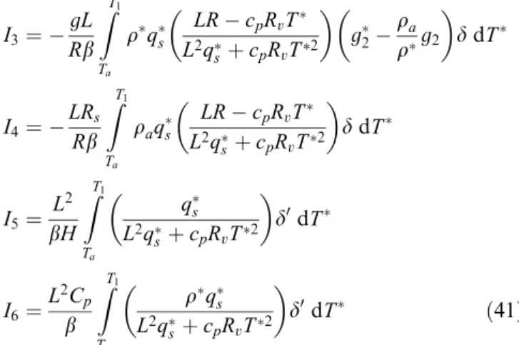
s L2_q

s ‡cpRvT2

d0dT …41†

whereT1is the temperature at 500 mb, andTais given by Eq. (19).

Since we will use 500 mb data to compute the integrals (41), P, T and q can be computed applying Eqs. (4) and (5) atzˆH1(500 mb height). Therefore, we obtain

P ˆ …500 mb† T1ÿb…HÿH1† T1

a

…42†

T ˆT1ÿb…HÿH1† …43†

Furthermore, q is computed from the perfect gas equation:

qˆP=RT …44†

UsingP,T andqfor 500 mb, we can computeq_aandTa

from Eqs. (18) and (19) respectively. The saturated speci®c humidity in the integrals (41) is given by Eq. (7), where the saturation vapor pressure is computed from Eq. (8) and the pressurePfrom Eq. (5). The densityq

is computed from Eq. (6).Rs is a function ofTa andT,

given by Eq. (27).

Finally the values of b, CD, g, L, R andRv, together with other values of parameter used in this work are shown in Table 1.

In order to obtain a linear formula for the anomalies of G5 similar to Clapp et al.'s (1965) Eq. (2), we have used normal values for the coecient of

Table 1.Model parameters

Symbol Value Units

Lapse rate b 6.5´₁₀)3 _Km)1 Drag coecient CD 1.5´10)3

Gravitational acceleration g 9.8 ms)2 Gas constant R 287.05 Jkg)1_K)1 Vapor gas constant Rv 461 Jkg)1K)1 Convection cumulus latent

heat release parameters

c

…ar†0

8.2´₁₀)4 0.025

Austausch coecient K 2.5´102 _ms)1 Vaporization latent

heat constant

L 2.47´₁₀6 _Jkg)1

Speci®c heat at constant pressure

cp 1.004 JK)1

J…h;T†, J…f;T†, r2_{T, E}

T, G2 and …TmaÿTm† in Eq.

(40). In agreement with conditions (13) and (14), theoretically d and d0 can be determined from a diagnostic formula for the vertical wind …W†, and from the conservation of water vapor equation. However since these equations are not contained explicitly in ATM, it is not possible to use this procedure. Therefore we have assumed arbitrarily

dˆd0ˆ1 in the integrals (41). This procedure could overvalue the precipitation in subsidence zones and/ or relative humidity below 100%. Taking into account these considerations, we have

G5ÿG5N ˆI1N f J h;T

0_ÿT0

N

ÿ

‡ PN

TNI2N‡I3N

J fÿ ;T0ÿT_N0

‡ g

cD V ! aN

f2 I4N‡KI6N 0

@

1

Ar2 _T0_ÿT0

N

ÿ

‡I5N‰…ET ÿETN† ‡…G2ÿG2N†Š

ÿ I5N‡ H1ÿh H0

A0ÿT0ÿT_N0 …45†

where the subscript N refers to normal or long period average values. In Eq. (45) we have assumed that the anomalies of Tma are negligibly small, and have used, according to Eq. (4),

Tmˆ

bH

2 ‡T ˆ

bH

2 ‡ T0‡T 0

… †:

Therefore T_m0 ˆT0 and T_m0 ÿT_mN0 ˆT0ÿT_N0 where

T_m0 ˆTmÿTm0, withTm0ˆbH=2‡T0.

Using Eqs. (31), (32) and (34) in Eq. (45) we obtain the following linear formula:

G5ÿG5N

… †_i;jˆa00ÿT_s0ÿT_sN0 _i;j‡b00ÿT0ÿT_N0_i;j

‡c00 @

@Y T

0_ÿT0

N

ÿ

i;j‡d

00 @ @X T

0_ÿT0

N

ÿ

i;j ‡e00r2ÿT0ÿT_N0_i;j …46†

where subscripts iand j, are index numbers identifying the X and Y map coordinates of a point in the NMC grid. Taking T0ÿT_N0 ˆT_DN0 , in Eq. (46), we obtain

@ @XT

0

DNi;jˆTDNi0 ‡1;jÿTDNi0 ÿ1;j

@ @YT

0

DNi;jˆTDNi0 ;j‡1ÿTDNi0 ;jÿ1

…47†

r2T_DNi0 _;jˆT_DNi0 _ÿ1;j‡T_DNi0 _;j‡1

‡T_DNi0 _‡1;j‡T_DNi0 _;jÿ1ÿ4T_DNi0 _;j

The coecients in Eq. (46) are given by:

a00ˆ I5N

1ÿkN

F32‡F₃₂0eN ‡ G002K2‡ 1ÿG002

ÿ K3 ÿ V ! aN h i

b00ˆ I5N

1ÿkN

F31ÿÿG00₂K2‡ÿ1ÿG00₂K3!VaN ÿA0 h i ÿ 1

1ÿkN

H1ÿh

H A0

c00ˆ 1

1ÿkN fx PN

TNI2N ‡I3N

‡I1Nhx f

M2

4D2 d00ˆ 1

1ÿkN fy

PN

TNI2N‡I3N

ÿI1Nhy f

M2

4D2

e00ˆ 1

1ÿkN

gCD!VaN

f2 I4N‡KI6N 0

@

1

AM2 D2

and

kN ˆI5N F300 ‡b3I

ÿ

d2

The coecienta00_{contains terms of longwave radiation} heating and sensible heating which are the surface temperature coecients in Eqs. (31) and (34).

The terms contained in b00 are the heating generated by longwave radiation, sensible heating and latent heat-ing release in convection cumulus activity; they are the coecients of 700 mb temperature in Eqs. (31), (34) and (37). a00 and b00 are coecients related to the second term in Eq. (12), therefore the ®rst and the second terms of the right side of Eq. (46) represents the latent heat release by non-adiabatic cooling of saturat-ed air.

The coecientsc00and d00are related to the ®rst and second terms of the right side of the vertical wind Eq. (29); and therefore, the third and the fourth terms in the right side of Eq. (46), represents the anomalies of precipitation due to the latent heat of saturated air induced by the terrain slope and by the divergence of geostrophic wind.

The coecient e00, contains the drag coecient CD

and the Austausch coecientK_{; therefore, the last term}

in the right side of Eq. (46) represents the anomalies of precipitation due to the latent heat release by adiabatic ascent of saturated air induced by surface friction, plus the latent heat release by non-adiabatic cooling of saturated air due to the divergence of horizontal turbulent ¯ux.

The shortwave radiation heating is included in the second term of the right side of thekN equation so it is

included in all coecients.

In the coecientsc00,d00 ande00,M is the map factor in a polar stereographic projection:

Mˆ 2

1‡sin/

where/ is the latitude angle,Dis the distance between consecutive points, fxˆ@f=@X, fy ˆ@f=@Y, hxˆ@h=@X, andhy ˆ@h=@Y, and where

@fi;j

@X ˆfi‡1;jÿfiÿ1;j;

@fi;j

@Y ˆfi;j‡1ÿfi;jÿ1

@hi;j

@X ˆhi‡1;jÿhiÿ1;j;

@hi;j

5 Numerical results

We assume that the statistical parametrization (Clapp

et al., 1965), which was developed using observed rainfall, temperature and wind data and where the coecients b, c and d were determinated by multiple correlation in a linear equation, is a good comparative equation to test our theoretical parametrization.

The coecients b0, c0 and d0 from Eq. (2) were determinated as functions of the formerb,candd. We computed those coecients and ourb00,c00and d00 from Eq. (46), in the NMC grid (Fig. 1), using mean-monthly normal values of temperature and height at 500 mb, obtained from the National Center of Atmospheric Research, (NCAR NMC Grid Point Data Set, CD-ROM) in winter and summer.

Fig. 2a±d.Geographical patterns of theb00_{coecient in the theoretical Eq. (46), and theb}0_{coecient in the Clappet al.(1965) formula, computed}

in 2 Wmÿ2_Kÿ1_.

The maps for the coecientsb00and b0 are shown in the Fig. 2a,b for January (winter), respectively, and for July (summer) in Fig. 2c,d, respectively.

The comparison of Fig. 2a,b shows some similarities in signs and magnitudes of the coecientsb00 andb0 for winter; however, in summer they are quite di€erent especially in ocean areas. We computed the correlation coecient (r), betweenb00andb0 ®elds and it is 0.62 for winter and 0.04 for summer.

In accordance with Fig. 2a,c, and the term

b00…T0ÿT_N0† in Eq. (46), above normal precipitation tends to occur with above normal temperature

‰…T0ÿT_N0†>0Šin high latitudes and with below normal temperature‰…T0ÿT_N0†<0Š at lower latitudes in winter and summer, except in the summer over the Arabian Sea, the Gulf of Bengal and the Tibet Plateau, where the above normal precipitation tends to occur with above normal temperature.

Fig. 3a±d.Geographical patterns of thec00_{coecient in the theoretical Eq. (46), and thec}0_{coecient, in the Clappet al.(1965) formula computed}

in 2 Wmÿ2_Kÿ1_.

The maps for the c00, c0; d00 and d0 coecients are shown for January (winter), in Figs. 3a, 3b, 4a and 4b, respectively, and for July (summer) in Figs. 3c, 3d, 4c and 4d, respectively.

From the geographic distribution of the coecientsc0

and d0, Clapp et al. (1965) concluded that these coecients depend mainly on terrain and latitude. Looking at ourc00,d00 winter maps, (Figs. 3a, 4a), there is a zero line crossing the map vertically in the case ofc00,

and crossing the map horizontally in the case ofd00. Due to the fact that the Coriolis parameter depends only on the latitude, the derivatives of …fx†_i;jˆfi‡1;jÿfiÿ1;j at

the grid points over the Y axis …80_{W† are zero;} similarly, the derivatives of …fy†i;jˆfi;j‡1ÿfi;jÿ1 at the

grid points over the X axis …10E† are zero. It can be seen in the maps of Figs. 3a and 4a where the zero isoline is along theY and X axes, respectively, with the exception of regions where orographic slopehxandhy is

Fig. 4a±d.Geographical patterns of thed00_{coecient in the theoretical Eq. (46), and thed}0_{coecient in the Clappet al.(1965) formula, computed}

in 2 Wmÿ2_Kÿ1_.

not zero. The statistical ®elds of Clapp et al.'s (1965)c0

and d0, (Figs. 3b, 4b) show the same characteristic zero isoline along 80_{W and 10E, respectively, and suggest} that the e€ect of the Coriolis parameter variation is present in these maps. The r coecient between the c00

and c0 ®elds is 0.64 and between thed00 and d0 ®elds is 0.72, for winter in both cases.

The summerc00 and d00 maps (Figs. 3c, 4c) are quite di€erent to the corresponding summer c0 and d0 maps

(Figs. 3d, 4d). The r coecients between the ®elds are 0.19 and )0.07 respectively. This di€erence may be

related to atmospheric phenomena which were not included in our parametrization.

The corresponding coecients to a00 and e00 do not exist in Eq. (2), and therefore we cannot compare these coecients. In the maps of winter and summer, (See Fig. 5) they are negative in the whole Northern Hemisphere and it is interesting to point out that above

Fig. 5a±d.Geographical patterns of thea00_ande00_{coecients in the theoretical Eq. (46), computed in 2 Wm}ÿ2

Kÿ1.aIs thea00_{coecient for}

normal precipitation occurs with negative values of

T_sDN0 ˆT_s0ÿT_sN0 for the case ofa00, and with also negative values ofT_s0ÿT_s0N ˆ r2_T0

DN for that ofe00. 6 Veri®cation experiments for the precipitation in Mexico

In order to compare the observed rainfall anomalies with the anomalies of the heat released by the conden-sation of water vapor in the clouds …G5ÿG5N†,

com-puted using our theoretical Eq. (46) and using Clapp

et al.'s (1965) formula, we carried out ®ve numerical experiments evaluating the contribution of the di€erent terms in our formula.

In these experiments we used 700 mb temperatures over a period of 36 months, from January 1981 to December 1983 and their corresponding normal values, both obtained from NCAR NMC Grid Point Data Set (CD-ROM) taking T0ÿT_N0 T7ÿT7N. The observed data for surface air temperature anomalies which are assumed to be equal to …T_s0ÿT_sN0 †, were obtained from the Servicio MeteoroloÂgico Nacional, Mexico. Further-more, we used observed precipitation and its average values also from the Servicio MeteoroloÂgico Nacional for the 36 months, at 97 stations scattered in Mexico and interpolated to 23 grid points of the NMC grid used in the ATM. The interpolation was made drawing by the monthly isohyets and their corresponding normal values for each month on the map of Mexico. The isohyets were drawn taking the orography into account, in other words, according to the orographic contour. The isolines were drawn through places of approximately same height, and then were determined by the precip-itation values in the 23 grid points over Mexico.

With Fc, we denote the computations using Clapp et al.'s (1965) formula, given by Eq. (2), which can be expressed as

…G5ÿG5N†_i;jˆb0ÿT0ÿT_N0_i;j‡c0 @ T

0_ÿT0

N

ÿ

@Y

i;j

‡d0 @ T

0_ÿT0

N

ÿ

@X

i;j

…48†

where the derivatives respect toY andX coordinates are given by Eq. (47).

F2denotes the experiment using our complete Eq. (46).

F3 refers to the experiment using in Eq. (46) the three terms similar to those of Clapp et al.'s (1965) formula, i.e., omitting the a00 and e00 terms; F4 denotes the experiment using Eq. (46), but omitting only thee00term, and ®nally F5 is an experiment where we have omitted only thea00term in Eq. (46).

Figure 6 shows an example to illustrate the di€erence between the similar equations of cases Fc and F3 over

Mexico. Figure 6a shows the percentage of normal precipitation observed in August of 1983 and Fig. 6b,c shows the corresponding computed values using casesFc

and F3 respectively.

The areas where the percentage of normal precipita-tion were above normal (100%) are shaded, and where they were below normal are in white. Comparison of the ®gures, shows that there is similarity in the percentage of normal precipitation between the observed precipitation (Fig. 6a) and theG5 anomalies computed in theF3 case (Fig. 6c), especially in the YucataÂn peninsula and Northern MeÂxico where it rains practically only in summer; in contrast, the map ofG5anomalies computed in theFccase has no similarity for this month, (Fig. 6b).

Table 2 shows the results of the experiments for the anomalies ofG5. In the second column are the percent-ages of sign correctly predicted for the 36 month period, evaluated by seasonal and annual averages forFc(using Clappet al.'s (1965) formula). In the next columns are shown the excesses of percentages overFcwhenF2,F3,F4

andF5 are used.

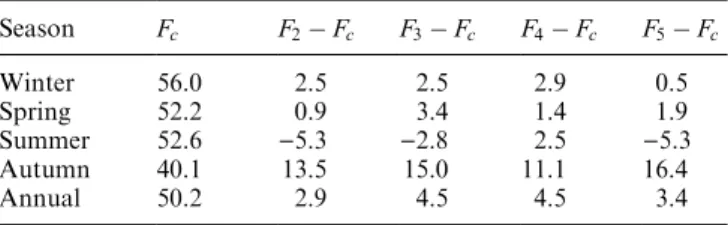
The experiments with the complete formula (F2), show an excess of percentage of sign correctly simulated with respect to those using Clappet al.'s (1965) formula (Fc) for the annual average and for all seasons, except in summer.

To determine the contribution of the di€erent terms in Eq. (46), we have carried out experimentsF3;F4 and F5.

In theF3case, when thea00ande00terms are neglected and Eq. (46) is similar to that of Clapp et al.'s (1965) Eq. (48), the greater percentage is positive in winter, spring and autumn but negative in summer. Comparison of theF3 case with the complete case…F2†shows that the

F3case gives a better estimation of the rainfall in spring, summer, autumn and in the annual average than the complete formula.

In theF4case the greater percentage is positive for all

seasons, and the annual average is the same than for the

F3 case and is 4.5%. Furthermore, the comparison of

…F4ÿFc†with …F3ÿFc†, shows that the inclusion of the

a00 term improves substantially the results in summer which is the rainy season in Mexico. The contribution of the terme00r2_T0_ÿT0

N†is seen comparing…F5ÿFc†with …F3ÿFc†. The results show that this term does not improve the estimation of the monthly rainfall anom-alies except in autumn, when the percentage of the F5

case is larger than that ofF3 case.

Table 2.Percentages in seasonal and annual averages of correctly

computed signs of the anomalies of precipitation computed in the

Fcexperiment, and compared to the results computed in theF2,F3,

F4 andF5 experiments

Season Fc F2ÿFc F3ÿFc F4ÿFc F5ÿFc

Winter 56.0 2.5 2.5 2.9 0.5

Spring 52.2 0.9 3.4 1.4 1.9

Summer 52.6 )5.3 )2.8 2.5 )5.3 Autumn 40.1 13.5 15.0 11.1 16.4

Fig. 6a±c.Percentage of normal precipitation in August 1983 in Mexico. The areas where the percentage is above 100% are shaded.a

7 Concluding remarks

1. In the annual average all our formulas show better results than that Clapp et al.'s (1965) one in the precipitation anomalies simulation.

2. It is important to notice that the F4 experiment, in which the surface temperature anomaly is included, besides the type of terms that appears in the Clappet al.'s (1965) formula and for the F3 formula (mid tropospheric temperature anomaly and its X and Y

derivatives), there is a signi®cant improvement in the estimation of rainfall in summer, the rainy season in Mexico. Therefore, this experiment suggests that the surface temperature anomaly may produce a better parametrization for this season.

3. A more sophisticated parametrization of precipitation than the one used in this work would not necessarily give an improvement in the estimation of the anom-alies of precipitation in the Northern Hemisphere and in particular in Mexico. However, the contribution to theG5 anomalies given by thec00andd00 terms in Eq. (46) could possibly be substantially improved, with a ®ner resolution in the computation of the orographic slope,hxandhy especially in Mexico's case. We think that it is possible to use a ®ner resolution nested grid, superposed on the NMC grid in mountain regions. 4. The assumption of geostrophic wind in Eq. (22), in

order to evaluate the rotational of wind stress, could be the reason that thee00r2_T0_ÿT0

N†term in Eq. (46)

does not improve the estimation of G5 anomalies. A more sophisticated parametrization of surface wind could be obtained, by introducing an angle between the wind and the isobars (Holton, 1972).

5. Another source of error could be to assumedˆd0ˆ1 in the integrals (41) which may overvalue the precip-itation at subsidence zones as in the arid zones of northern Mexico.

We think that these measures in (3), (4) and (5), would improve the calculation of the coecientsc00,d00

and e00 and maybe the correlation coecient between our c00 d00 and their corresponding c0, d0, Clapp et al.'s (1965) coecients will be increased in summer, and it would improve the results of the summer season in Table 2.

6. At present, there are improved precipitation and temperature data so that other alternatives are:

To use the statistical Clappet al. (1965) formula in the form of

RDN ˆbT7DN‡cU7DN‡dV7DN

without using the thermal wind hypothesis. In this case it is necessary to have a model to predict explicitlyU7DN

and V7DN:. In the case of a model which predicts only

T7DN (as ATM does), another option is to search for a

statistical formula in the form of

G5DN ˆb0T7DN‡c0@T7DN

@x ‡d

0@T7DN @y

with linear regression coecientsb0,c0and d0 recast.

Another alternative is to use Adem's water vapor conservation parametric method described in a previous paper (Adem, 1968a).

Finally, in future work we will verify our formula in other continental and oceanic areas, as well as in the total region of integration of the NMC grid, using the best available data.

Acknowledgements.The authors would like to thank E. E. Villanu-eva for fruitful discussions and Alejandro Aguilar Sierra for computational support. The Editor in Chief thanks A. Berger and another referee for their help in evaluating this paper.

References

Adem, J., On the physical basis for the numerical prediction of

monthly and seasonal temperatures in the troposphere-ocean-continent system,Mon. Weather Rev.,92,91±103, 1964.

Adem, J.,Experiments aiming at monthly and seasonal numerical

weather prediction,Mon. Weather Rev.,93,495±503, 1965.

Adem, J.,Parametrization of atmospheric humidity using

cloud-iness and temperature,Mon. Weather Rev.,95,83±88, 1967a.

Adem, J., Relations among wind, temperature, pressure, and

density, with particular reference to monthly averages, Mon. Weather Rev.,95,531±539, 1967b.

Adem, J., A parametric method for computing the mean water

budget of the atmosphere,Tellus,20,621±632, 1968a.

Adem, J., Long range numerical prediction with a time average

thermodynamical model. Part 1) the basic equations,Internal report of Extended Forecast Division, NMC, Weather Bureau, ESSA, Washington D.C. (Available on request to Centro de Ciencias de la AtmoÂsfera, UNAM, 04510 MeÂxico D.F., MeÂxico), 1968b.

Adem, J., On the seasonal e€ect of orbital variations on the

climates of the next 4000 years.Annales Geophysicae,14,1198± 1206, 1996.

Adem, J., and Donn, W. L.,Progress in monthly climate forecasting

with a physical model. Bull. Am. Meteorol. Soc.,62,1666±1675, 1981.

Adem, J., Ruiz, A., Mendoza, V. M., GardunÄo, R., and Barradas, V.,

Recent experiments on monthly weather prediction with the Adem thermodynamic climate model, with special emphasis on Mexico,AtmoÂsfera,8,23±34, 1995.

Clapp, P. F., Scolnik, S. H., Taubensee, R. E., and Winningho€, F. J., Parametrization of certain atmospheric heat sources and sinks for use in a numerical model for monthly and seasonal forecasting,Internal Report, Extended Forecast Division, (Avail-able on request to Climate Analysis Center NWS/NOAA, Washinton D.C., 20233), 1965.

Holton, J. R.,An introduction to dynamic meteorology, Academic

Press, New York N.Y., pp. 319, 1972.

Kasahara, A., and Washington, W. M., NCAR global general

circulation model of the atmosphere,Mon. Weather Rev., 95,

389±402, 1967.

Kuo, H. L.,On formation and intensi®cation of tropical cyclones

through latent heat release by cumulus convection,J. Atmos. Sci.,22,40±63, 1965.

Krishnamurti, T. N.,An experiment in numerical prediction in the

equatorial latitudes,Q. J. R. Meteorol. Soc.,95,594±620, 1969.

Mendoza, V. M.,Un Modelo TermodinaÂmico del Clima, Facultad

de Ciencias, UNAM, MeÂxico D.F., MeÂxico, pp. 184, (Ph D Thesis), 1992.

Negri, A. J., Adler, R. F., Maddox, R. A., Howard, K. W., and

Keehn, P. R.,A regional rainfall climatology over Mexico and

the southwest United States derived from passive microwave and geosynchronous infrared data,J. Clim.,6,2144±2161, 1993.

Washington, W. M., and Williamson, D. L.,A description of the