High resolution land surface modeling utilizing remote sensing parameters and the Noah-UCM: a case study in the Los Angeles Basin

(1)

HESSD

11, 7469–7511, 2014

High resolution land surface modeling

utilizing remote sensing parameters

P. Vahmani and T. S. Hogue

Title Page

Abstract Introduction

Conclusions References

Tables Figures

◭ ◮

Back Close

Full Screen / Esc

Printer-friendly Version

Interactive Discussion

Discussion

P

a

per

|

Discus

sion

P

a

per

|

Discussion

P

a

per

|

Discussion

P

a

per

|

Hydrol. Earth Syst. Sci. Discuss., 11, 7469–7511, 2014 www.hydrol-earth-syst-sci-discuss.net/11/7469/2014/ doi:10.5194/hessd-11-7469-2014

This discussion paper is/has been under review for the journal Hydrology and Earth System Sciences (HESS). Please refer to the corresponding final paper in HESS if available.

High resolution land surface modeling

utilizing remote sensing parameters and

the Noah-UCM: a case study in the Los

Angeles Basin

P. Vahmani1and T. S. Hogue2,1

1

University of California, Los Angeles, CA, USA 2

Colorado School of Mines, Golden, CO, USA

Received: 27 April 2014 – Accepted: 13 June 2014 – Published: 4 July 2014

Correspondence to: T. S. Hogue ([email protected])

(2)

HESSD

11, 7469–7511, 2014

Title Page

Tables Figures

◭ ◮

Back Close

Full Screen / Esc

Discussion

P

a

per

|

Discus

sion

P

a

per

|

Discussion

P

a

per

|

Discussion

P

a

per

|

Abstract

In the current work we investigate the utility of remote sensing based surface pa-rameters in the Noah-UCM (urban canopy model) over a highly developed urban area. Landsat and fused Landsat-MODIS data are utilized to generate high res-olution (30 m) monthly spatial maps of green vegetation fraction (GVF), impervi-5

ous surface area (ISA), albedo, leaf area index (LAI), and emissivity in the Los Angeles metropolitan area. The gridded remotely sensed parameter datasets are directly substituted for the land-use/lookup-table values in the Noah-UCM model-ing framework. Model performance in reproducmodel-ing ET (evapotranspiration) and LST (land surface temperature) fields is evaluated utilizing Landsat-based LST and ET 10

estimates from CIMIS (California Irrigation Management Information System) sta-tions as well as in-situ measurements. Our assessment shows that the large de-viations between the spatial distributions and seasonal fluctuations of the default and measured parameter sets lead to significant errors in the model predictions of monthly ET fields (RMSE=22.06 mm month−1). Results indicate that implemented 15

satellite derived parameter maps, particularly GVF, enhance the Noah-UCM capabil-ity to reproduce observed ET patterns over vegetated areas in the urban domains (RMSE=11.77 mm month−1). GVF plays the most significant role in reproducing the observed ET fields, likely due to the interaction with other parameters in the model. Our analysis also shows that remotely sensed GVF and ISA improve the model capability 20

to predict the LST differences between fully vegetated pixels and highly developed ar-eas. However, the model still underestimates remotely sensed LST values over highly developed areas. We hypothesize that the LST underestimation is due to structural formulation in the UCM and cannot be immediately solved with available parameter choices.

(3)

HESSD

11, 7469–7511, 2014

Title Page

Tables Figures

◭ ◮

Back Close

Full Screen / Esc

Discussion

P

a

per

|

Discus

sion

P

a

per

|

Discussion

P

a

per

|

Discussion

P

a

per

|

1 Introduction

Urbanization introduces significant changes to land surface characteristics that ulti-mately perturb land–atmosphere fluxes of sensible heat, latent heat, and momen-tum which, in turn, alter atmospheric properties as well as local weather and climate (Landsberg, 1981; Kalnay and Cai, 2003; Miao et al., 2009; Ridder et al., 2012). Ur-5

ban surfaces are covered with variety of materials with distinct thermal, radiative, and moisture properties influencing surface energy and water budgets (Arnfield, 2003). Moreover, contrasting aerodynamic properties of buildings significantly change surface roughness (Cotton and Pielke, 1995). The effects associated with modified urban land-scapes extend to air quality (Taha et al., 1997), local temperatures (Bornstein, 1987; 10

Van Wevenberg et al., 2008), local and regional atmospheric circulation (Pielke et al., 2002; Marshall et al., 2004; Niyogi et al., 2006), and regional precipitation patterns (Changnon and Huff, 1986; Changnon, 1992; Lowry, 1998).

Mesoscale meteorological models have been increasingly applied over urban areas to examine the urban–atmosphere exchange of heat, moisture, momentum or pollu-15

tants. Recently updated parameterization in the community Weather Research and Forecasting (WRF) model includes coupling between the Noah LSM (Land Surface Model) and a single layer urban canopy model (UCM) (Kusaka et al., 2001; Kusaka and Kimura, 2004) which has substantially advanced the understanding and modeling of the mesoscale impact of cities. The coupled WRF-Noah-UCM has been applied to 20

major metropolitan regions around the world (e.g, Houston, Beijing, Guangzhou/Hong Kong, Salt Lake City, and Athens) to better understand the contribution of urbanization to changes in urban heat island, surface ozone, horizontal convective rolls, boundary layer structure, contaminant transport and dispersion, and heat wave events (Chen et al., 2004; Jiang et al., 2008; Miao and Chen, 2008; Miao et al., 2009; Wang et al., 25

(4)

HESSD

11, 7469–7511, 2014

Title Page

Tables Figures

◭ ◮

Back Close

Full Screen / Esc

Discussion

P

a

per

|

Discus

sion

P

a

per

|

Discussion

P

a

per

|

Discussion

P

a

per

|

et al., 2010; Chen et al., 2011). Although realistic representation of surface properties is critical for accurate simulation of the physical processes occurring in urban regions, the majority of previous modeling studies rely on traditional land-use data and lookup tables to define surface parameters.

Remote sensed observations provide important spatial information on urban-induced 5

physical modifications to the Earth’s surface (Jin and Shepherd, 2005). Airborne LI-DAR (Light Detection and Ranging) systems and photogrammetric techniques have been utilized to produce morphological parameters over urban areas (Burian et al., 2004, 2006, 2007; Taha, 2008; Ching et al., 2009). Burian et al. (2004) used airborne LIDAR data, at 1 m resolution, to generate datasets of 20 urban canopy parameters 10

(e.g., building height, height-to-width ratio, and roughness length) for an air quality modeling study over Houston, Texas. Tahah (2008) introduced an alternative and low-cost approach for generating urban canopy parameters input for the uMM5 over Sacra-mento region, California. The study relied on commercially available Google Earth PRO imagery to generate urban geometry parameters (e.g., pavement land-cover fraction, 15

roof cover fraction, and mean building height). Using LIDAR-based three-dimensional data sets of buildings and vegetation, Ching et al. (2009) presented a high-resolution database of the geometry, density, material, and roughness properties of the morpho-logical features for applications in WRF and other models over Houston, Texas. While promising, the availability of such datasets is currently limited to a few geographical 20

locations and the reproduction of such datasets is extremely challenging due to high collection costs and data management difficulties associated with the extremely large size of LIDAR datasets (Burian et al., 2006; Ching et al., 2009).

Observations from satellites, on the other hand, have been utilized in model valida-tion processes over urban areas (Miao et al., 2009; Giannaros et al., 2013). In addivalida-tion 25

(5)

HESSD

11, 7469–7511, 2014

Title Page

Tables Figures

◭ ◮

Back Close

Full Screen / Esc

Discussion

P

a

per

|

Discus

sion

P

a

per

|

Discussion

P

a

per

|

Discussion

P

a

per

|

simulated LST distribution in Beijing. Other studies have employed satellite data to re-place outdated urban land use maps in atmospheric models with new remote sensing products (Cheng and Byun, 2008; Cheng et al., 2013). Focusing on boundary later mix-ing conditions and local wind patterns in the Houston Ship channel, Cheng and Byun (2008) reported that the Noah LSM and planetary boundary layer (PBL) scheme per-5

formances in the MM5 were improved when land-use type distributions were correctly represented in the model using high resolution Landsat-based land use data. Cheng et al. (2013) compared WRF simulations in the Taiwan area using US Geological Sur-vey (USGS), MODIS, and SPOT (Système Pour l’Observation de la Terre) based land use data. Using the new high resolution land use types obtained from SPOT satel-10

lite imagery, the WRF predictions of daytime temperatures and onshore sea breezes had the best agreement with observed data. Furthermore, more accurate surface wind speeds were simulated when MODIS and SPOT data replaced conventional USGS land use maps in the WRF runs due to the more realistic representation of roughness length in the remotely sensed databases. Although these and other previous studies 15

(e.g., Jin and Shepherd, 2005) have recognized the usefulness of satellite imagery (e.g., NASA’s Terra, Aqua, and Landsat data) in specifying surface physical character-istics in urban environments, very few have directly incorporated high resolution grid-ded satellite-based parameters (e.g., impervious surface area, albedo, and emissivity) into parameter estimation within land surface/atmospheric modeling systems.

20

In the current work we investigate the utility of remote sensing based surface pa-rameters in the Noah-UCM modeling framework over a highly developed urban area. Among parameters that can be related to a measurable physical quantity, we eval-uate those routinely and freely obtained from satellite-based platforms. The derived parameter sets are implemented in the Noah-UCM with a focus on simulated surface 25

(6)

HESSD

11, 7469–7511, 2014

Title Page

Tables Figures

◭ ◮

Back Close

Full Screen / Esc

Discussion

P

a

per

|

Discus

sion

P

a

per

|

Discussion

P

a

per

|

Discussion

P

a

per

|

area. The temporal and spatial distributions of newly assigned parameters are com-pared with those based on the model lookup tables. Next, gridded remotely sensed parameter datasets are directly incorporated into the Noah-UCM modeling framework replacing the land-use/lookup-table values. The sensitivity of the simulated energy and water fluxes to the newly developed spatial metrics of parameters is presented. The 5

model’s performance in reproducing evapotranspiration (ET) and LST fields is evalu-ated utilizing Landsat-based land surface temperature and ET estimates from CIMIS (California Irrigation Management Information System) stations as well as in-situ mea-surements. Finally, the influence of each parameter set on the urban energy and water budgets is investigated.

10

2 Study area

The study domain is a 49 km2 highly developed neighborhood in the City of Los An-geles (Fig. 1). Los AnAn-geles is the second most populous city in the United States with a population of 3.8 million (US Census, 2011), covering an area of 1215 km2in South-ern California. The city has a mediterranean climate and receives 381 mm of annual 15

precipitation, mostly over the winter months (NOAA-CSC, 2003; SCDWR, 2009). Due to the semi-arid nature of the region, the city’s water supply is heavily dependent on im-ported water (52 % from the Colorado River and 36 % from the Los Angeles Aqueduct) (LADWP, 2010). Regional water demands and the extensive dependence on external sources make accurate spatial representation of the metropolitan area in regional land 20

(7)

HESSD

11, 7469–7511, 2014

Title Page

Tables Figures

◭ ◮

Back Close

Full Screen / Esc

Discussion

P

a

per

|

Discus

sion

P

a

per

|

Discussion

P

a

per

|

Discussion

P

a

per

|

3 Remotely sensed parameters

Remote sensing data are retrieved from Landsat ETM+ images with a nominal pixel resolution of 30 m in the short wave bands and 60 m in the thermal band. The level 1Gt ETM₊imagery from USGS EROS, spanning years 2010–2011, are calibrated and atmospherically corrected through the Landsat Ecosystem Disturbance Adaptive Pro-5

cessing System (LEDAPS). Study domain data are not affected by the failure of the Landsat-7 ETM+ Scan Line Corrector in 2033 (SLC-off). Employing a knowledge-based approach, similar to the one introduced by Song and Civco (2002), several binary masks are applied to the images to detect contaminated areas (cloud and shadow). Images with cloud and/or shadow are distinguished and omitted in the fol-10

lowing parameter retrievals. A total of 24 pure images, acquired over two years, are utilized in the parameter estimation processes.

In addition to Landsat observations, MODIS products from Terra and Aqua satel-lite platforms are also utilized. The MODIS MCD43A BRDF (Bidirectional Reflectance Distribution Function) products, concurrent with pure Landsat images, are collected for 15

use in the parameter calculations. The 500 m BRDF products are generated by the MODIS Adaptive Processing System (MODAPS) at the Goddard Space Flight Center (GSFC), using a kernel-driven linear model, and distributed through the Land Pro-cesses DAAC (Distributed Active Archive Center) (Justice et al., 2002; Schaaf et al., 2002; Shuai et al., 2008). The described Landsat and MODIS-based data are used to 20

produce a group of six remotely sensed derivatives:

– Green Vegetation Fraction (GVF): GVF spatial maps are derived according to Gutman and Ignatov (1998) utilizing NDVI (Normalized Difference Vegetation In-dex) measurements. First, atmospheric corrected reflectance values from the red (ρETM3) and near-infrared (ρETM4) bands of Landsat ETM+ are used to derive 25

(8)

HESSD

11, 7469–7511, 2014

Title Page

Tables Figures

◭ ◮

Back Close

Full Screen / Esc

Discussion

P

a

per

|

Discus

sion

P

a

per

|

Discussion

P

a

per

|

Discussion

P

a

per

|

NDVI=ρ_ρETM4−ρETM3 ETM4+ρETM3

(1)

GVF₌ NDVI−NDVIo

NDVI_∞−NDVI_o (2)

where NDVI_o and NDVI_∞are constant values computed using signals from bare soil and densely vegetated pixels in the study domain, respectively.

5

– Impervious Surface Area (ISA):ISA is shown to be inversely proportional to veg-etation fraction where non-vegetated pervious surfaces are rare (Bauer et al., 2007). Since the majority of pervious surfaces in the studied domain are vege-tated and heavily irrigated throughout the year, ISA is assumed to be the comple-ment of the vegetation fraction:

10

ISA=(1−GVF_max)×100 (3)

where GVFmaxis the maximum GVF detected over the two year study period. The produced ISA map shows high accuracy (>95 %) when compared to a previously developed high resolution land cover map, based on QuickBird remote sensing 15

data, aerial photographs, and geographic information systems over the city of Los Angeles (McPherson et al., 2008).

– Albedo:employing a recent methodology by Shuai et al. (2011), 30 m land surface albedo maps is generated utilizing Landsat surface reflectance and anisotropy information from concurrent 500 m MODIS BRDF products. Landsat data are re-20

projected from UTM to MODIS sinusoidal projection and aggregated from 30 m to 500 m. Using USGS-based land cover types, the percentage of each land cover class within each MODIS pixel is computed, then relatively pure pixels (>85 % purity) are selected for each class. MCD43A2 quality assessment product is used to choose highest quality MODIS MCD43A1 BRDF parameters for the pure pix-25

(9)

HESSD

11, 7469–7511, 2014

Title Page

Tables Figures

◭ ◮

Back Close

Full Screen / Esc

Discussion

P

a

per

|

Discus

sion

P

a

per

|

Discussion

P

a

per

|

Discussion

P

a

per

|

sky albedo, and black sky albedo under the solar geometry at Landsat overpass time and MODIS scale. Next, the spectral albedo-to-nadir reflectance ratios, for white sky and black sky albedos, are calculated over the pure pixels. The resul-tant ratios, specific to each land cover class, are applied to Landsat surface re-flectance to generate the spectral white sky and black sky albedos for each Land-5

sat pixel. A further narrowband-to-broadband conversion based on extensive ra-diative transfer simulations by Liang (2000) is applied to generate the broadband albedos at shortwave regime. Finally, albedo (blue sky) is modeled as an inter-polation between the black sky (αbs) and white sky (αws) albedos as a function of the fraction of diffuse skylight (S(θ,τ(λ)) which is estimated by the 6S (Second 10

Simulation of the Satellite Signal in the Solar Spectrum) codebase (Eq. 4) (Schaaf et al., 2002).

α(θ,λ)={1−S(θ,τ(λ))}αbs(θ,λ)+S(θ,τ(λ))αws(θ,λ) (4)

whereτ,θ, andλare optical depth, solar zenith, and wavelength, respectively. 15

– Leaf Area Index (LAI):Stenberg et al. (2004) showed that a reduced simple ratio (RSR) explains 63–75 % of the variations in LAI and that maps of projected LAI, based on RSR, have good agreement with observations. In the current study, LAI values are retrieved based on the LAI-RSR correlations which are specified utiliz-ing table-based LAI estimates in pure (fully vegetated) pixels and remotely sensed 20

RSR maps. The atmospheric corrected reflectance values of Landsat ETM spec-tral channels red (ρETM3), near infrared (ρETM4), and mid infrared (ρETM5), imple-mented in the following equation (Eq. 5), define RSR:

RSR=ρ_ρETM4 ETM3

×ρ5max−ρETM5

ρ5_max+ρ5_min

(5) 25

(10)

HESSD

11, 7469–7511, 2014

Title Page

Tables Figures

◭ ◮

Back Close

Full Screen / Esc

Discussion

P

a

per

|

Discus

sion

P

a

per

|

Discussion

P

a

per

|

Discussion

P

a

per

|

– Emissivity: among various methods developed to define land surface emissiv-ity, the NDVI Thresholds Method (NDVITHM) has been widely applied to urban areas (Stathopoulou and Cartalis, 2007; Stathopoulou et al., 2007; Tan and Li, 2013). NDVITHMis superior to other methods since the consideration of the inter-nal reflections (cavity effects), caused by heterogeneous surfaces minimizes the 5

overall error in this approach (Sobrino et al., 2001). This methodology, originally introduced by Sobrino and Raissouni (2000) and modified later by Stathopoulou et al. (2007) for urban areas, is selected for land surface emissivity estimation in the current work. Using the Landsat-based NDVI thresholds, the study area is divided into four classes: (1) fully vegetated (NDVI>0.5), (2) built-up areas with 10

sparse vegetation (NDVI≤0.2), (3) mixture of man-made material and vegetation (NDVI>0.2 and≤0.5), and (4) water bodies (NDVI<0). Mean emissivity values of 0.98, 0.92, and 0.995 are then used for fully vegetated, built-up and water pix-els (similar to Tan and Li, 2013). Emissivity values (ε) for mixed pixels (class 3) are estimated using the following equations (for details see Stathopoulou et al., 15

2007):

ε=0.017PV+0.963 (6)

PV=

(NDVI−0.2)2

(0.5−0.2)2 . (7)

– Land Surface Temperature (LST):the emissivity corrected land surface tempera-20

ture (LST) is calculated as follows (Artis and Carnahan, 1982):

LST= BT

{1+(λ×_ρBT×lnε)} (8)

where BT is Landsat at sensor brightness temperature (K);λandεare the wave-length of emitted radiance (11.5 µm) and surface emissivity; ρ=hc/σ (1.438× 25

(11)

HESSD

11, 7469–7511, 2014

Title Page

Tables Figures

◭ ◮

Back Close

Full Screen / Esc

Discussion

P

a

per

|

Discus

sion

P

a

per

|

Discussion

P

a

per

|

Discussion

P

a

per

|

4 Numerical modeling system

4.1 Noah LSM-UCM Model

Land surface processes are parameterized using the o_ffline Noah LSM (Chen and Dudhia, 2001) coupled with the single layer UCM (Kusaka et al., 2001; Kusaka and Kimura, 2004). The Noah LSM is based on a diurnally dependant Penman potential 5

evaporation approach, a multi-layer soil parameterization, a canopy resistance model, surface hydrology, and frozen ground physics (Chen et al., 1996, 1997; Chen and Dudhia, 2001; Ek et al., 2003). The UCM parameterization includes urban building geometry, shadowing from buildings, reflections and trapping of radiation in a street canyon, and an exponential wind profile. The Noah LSM provides surface sensible and 10

latent heat fluxes and surface skin temperature for vegetated areas (e.g., parks and trees) and the UCM calculates the fluxes for impervious surfaces. The outputs from the Noah LSM and UCM are coupled through the urban surface fractions.

4.2 Irrigation module

Irrigation is accounted for, in the Noah-UCM modeling framework, by incorporating an 15

urban irrigation module developed in our previous work (Vahmani and Hogue, 2013, 2014). The developed irrigation scheme mimics the effects of urban irrigation by in-creasing soil moisture content in vegetated portion of grid pixels at a selected interval. Added anthropogenic soil moisture contribution is a function of the soil moisture deficit, which is the difference between irrigated soil moisture content and actual soil moisture 20

(12)

HESSD

11, 7469–7511, 2014

Title Page

Tables Figures

◭ ◮

Back Close

Full Screen / Esc

Discussion

P

a

per

|

Discus

sion

P

a

per

|

Discussion

P

a

per

|

Discussion

P

a

per

|

SMC_IRR₌α×SMC_max (9)

DEF=max{[SMC_IRR−SMC₁], 0} (10)

IRR₌ρw

∆tDEF×D1 (11)

where saturation soil moisture content (SMCmax; m 3

m−3) and irrigation demand factor 5

(α; unit less) define irrigated soil moisture content (Eq. 9);D1is top soil layer thickness (10 cm);ρw(kg m

−3

) and∆tstand for water density and Noah-UCM time step (3600 s), respectively. The parameter α, ranging from zero to one, regulates the amount of ir-rigation water added to the soil each time the scheme increases the soil moisture, simulating an irrigation event. Similar to previous studies (Hanasaki et al., 2008a, b; 10

Pokhrel et al., 2012) an irrigation demand factor of 0.75 is utilized in the current work. The irrigation interval is set to three times per week according to the water restrictions implemented by Los Angeles Depart, 2013).

4.3 Land cover data and forcing fields

The Noah-UCM modeling system requires static data to describe physical character-15

istics of the surface, including soil type, slope type, vegetation type, and urban type. A combination of the Soil Data Mart (http://soildatamart.nrcs.usda.gov) and the Los Angeles Department of Public Works (LADPW) databases are used to gather soil classification information. Land use and land cover are parameterized using the 30 m NOAA C-CAP-2006 land cover data which is transformed to urban and vegetation type 20

spatial maps over the study domain. High, medium, and low intensity developed land cover types, recognized by NOAA, are converted to UCM Industrial/Commercial, high and low intensity residential types, respectively. The developed open space along with natural land types are categorized as one of the 27 Noah LSM vegetation classes.

The offline Noah LSM-UCM is forced utilizing hourly ground-based observations 25

(13)

HESSD

11, 7469–7511, 2014

Title Page

Tables Figures

◭ ◮

Back Close

Full Screen / Esc

Discussion

P

a

per

|

Discus

sion

P

a

per

|

Discussion

P

a

per

|

Discussion

P

a

per

|

1 January 2010 to 31 December 2011. There are ten CIMIS and eight NCDC stations within close proximity of the study domain (Fig. 1a). The NCDC stations, which use Au-tomated Surface Observing Systems (ASOS), are located at smaller local airports (6 stations), one major airport (Los Angeles International Airport), and a university cam-pus (University of Southern California; USC) within the Los Angeles metropolitan area. 5

Reporting the meteorological conditions, the NCDC stations are used for wind speed, air temperature, relative humidity, air pressure, and incoming long wave radiation. All NCDC data are gathered at a standard reference height of 2 m. The regional CIMIS stations are utilized for solar radiation (using LI200S pyranometer) and tipping bucket rain gauges in 18 stations (NCDC and CIMIS) are included in collection of precipitation 10

data. Inverse-distance weighting (2nd power) is employed to create the spatial grid-ded forcing fields. Linear interpolation and data from the nearest gage are utilized to replace missing data.

5 Numerical experiments and evaluation methods

5.1 Remote sensing based parameterization

15

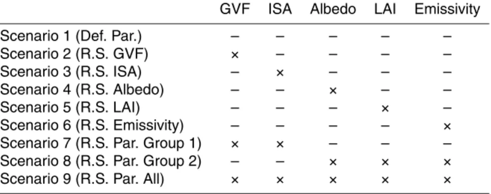
To investigate the sensitivity of the Noah-UCM model to integration of the developed remotely sensed parameters, nine simulation scenarios are designed (Table 1). A con-trol experiment (scenario 1) is conducted in which all default parameters are utilized in the Noah-UCM. Scenarios 2 to 6 explicitly assess each individual parameter effects on urban energy and water budgets using the newly incorporated remote sensing param-20

eters. Scenario 7 analyzes the effects of employing both remotely sensed GVF and ISA while scenario 8 assesses simultaneous integration of albedo, LAI, and emissivity. We are interested in the comparison of scenarios 7 and 8 as the Noah-UCM parameteriza-tions use GVF and ISA to select albedo, LAI, emissivity, and roughness length values from the predefined ranges in the parameter tables. It is worth mentioning that GVF al-25

(14)

HESSD

11, 7469–7511, 2014

Title Page

Tables Figures

◭ ◮

Back Close

Full Screen / Esc

Discussion

P

a

per

|

Discus

sion

P

a

per

|

Discussion

P

a

per

|

Discussion

P

a

per

|

length and building height over the impervious surfaces are kept at the default values listed by Chen et al. (2011). Scenarios 7 and 8 help quantify the contribution of each parameter group to the model’s ability to reproduce the observed surface states and fluxes. Finally, the last experiment (scenario 9) implements all five remotely sensed pa-rameter sets in the simulations. It should be noted that the GVF and LAI measurements 5

over mixed pixels (vegetated urban areas) are scaled up using urban fractions since, in the Noah-UCM modeling framework, these parameters characterize only the pervious portion (1 – urban fraction) of each pixel. Other than the implemented remote sending based parameters, the rest of the model parameters are kept at default values. All ex-periments incorporate the irrigation module and irrigation rates are kept constant in all 10

scenarios. All scenarios are run at 30 m spatial and 1 h temporal resolutions, spanning 2010 and 2011, with the first three months used as model initialization.

5.2 Model evaluation approach

In order to evaluate the performance of the Noah-UCM modeling framework, simu-lated LSTs are compared with concurrent Landsat observations and simusimu-lated la-15

tent heat flux time series are assessed against CIMIS-based ET observations. The CIMIS network was established in 1982 by the CDWR (California Department of Water Resources) and the University of California at Davis in order to provide real-time weather conditions and irrigation water need estimates for California’s agricul-tural community. The automated CIMIS stations measure hourly surface solar radia-20

tion, temperature, humidity, wind, precipitation, soil temperature, and surface pressure (http://www.cimis.water.ca.gov). Employing observed meteorological fields over a well-watered soil, the reference ET (ET0) is calculated for each site. Utilizing a methodology introduced by CDWR (2000), actual urban landscape ET is estimated using ET₀ and a landscape coefficient, which is a function of species, density, and microclimate fac-25

(15)

HESSD

11, 7469–7511, 2014

Title Page

Tables Figures

◭ ◮

Back Close

Full Screen / Esc

Discussion

P

a

per

|

Discus

sion

P

a

per

|

Discussion

P

a

per

|

Discussion

P

a

per

|

need categories (i.e., low, moderate, and high), a value from high category is selected (average species factor=0.80). Assuming the “average” category for vegetation den-sity, a density factor of 1 is used. Furthermore, a “high” category of microclimate condi-tion is used (microclimate factor=1.25) for the current highly developed study domain. This factor is utilized to take into account the contribution of the developed surfaces 5

to the water loss from vegetated areas, through anthropogenic heating, reflected light, and high temperatures of surrounding heat-absorbing surfaces (e.g., paving and build-ings). Using these factors, a landscape coefficient of 1 (landscape coefficient=species factor×density factor×microclimate factor) is prescribed. This coefficient and ET0 es-timations from ten CIMIS stations within close proximity of the study domain (Fig. 1a) 10

are utilized to compute the urban landscape ET which is then used in validation pro-cesses of the Noah-UCM. ET output of the model is also evaluated against recent ET measurements in the greater Los Angeles area (Moering, 2011). Moering (2011) employed a previously developed chamber approach to measure instantaneous ET in an irrigated and a non-irrigated park in the Los Angeles metropolitan area during WY 15

(Water Year) 2011 (WY is defined as 1 October the previous year to 30 September the designated year). They reported an annual ET of about 1224 mm over the observed irrigated park, which is located within our study domain.

6 Sensitivity study of surface parameters

6.1 Temporal evaluation

20

The monthly time series of the default Noah-UCM and remote sensing based GVF, ISA, albedo, and LAI are compared and modeled cumulative monthly sensible and latent heat fluxes, using default and newly estimated parameters, are presented over fully vegetated, low intensity residential, and industrial/commercial areas (Fig. 2). Fluxes from high intensity residential areas are not presented as they behave similarly to those 25

(16)

HESSD

11, 7469–7511, 2014

Title Page

Tables Figures

◭ ◮

Back Close

Full Screen / Esc

Discussion

P

a

per

|

Discus

sion

P

a

per

|

Discussion

P

a

per

|

Discussion

P

a

per

|

significantly increased throughout the year when remote sensing products are utilized (Fig. 2a). Moreover, the default seasonal variations of GVF values, assumed over all the land cover types, are not detected in Landsat imagery (Fig. 2a). The reason for this is the significant and year round irrigation in the Los Angeles area, which is not accounted for in the default parameter tables. This is confirmed by previous studies (Johnson and 5

Belitz, 2012) that reported urban vegetation supported by water delivery, in contrast to common seasonal behavior of greening in the winter/spring and browning in the sum-mer, maintains constant greenness which is reflected in NDVI and GVF estimates. GVF plays a dominant role in the Noah-UCM simulations as it defines the vegetated fraction of the natural areas, and specifies albedo, LAI, emissivity, and roughness length values 10

from the predefined ranges in the model lookup tables. Furthermore, GVF partitions the total ET between soil direct and canopy ET. The simulated latent heat flux is consider-ably decreased (up to 139 MJ m−2month−1) in the summer time and increased over the remaining months, when remotely sensed GVF is incorporated in the fully vegetated areas (Fig. 2b). Since any increase of latent heat flux that does not alter the radiative 15

balance leads to a reduction in sensible flux, the newly developed GVF values, in turn, cause enhancements (up to 103 MJ m−2month−1) in the simulated summer sensible heat fluxes and a reduction in the sensible heat fluxes during the remaining months (Fig. 2b). Latent and sensible heat fluxes from the low intensity residential pixels show similar but less significant changes (up to 66.1 and 31.0 MJ m−2 per month, respec-20

tively), when the new parameter sets are implemented. Adding remotely sensed GVF causes insignificant changes in the industrial/commercial area fluxes due to the small percentage of vegetated land cover in such areas (Fig. 2d).

There are also large deviations between the look-up-table ISAs and the remotely sensed values. Averaged ISA is decreased (10 %) over industrial and commercial pix-25

(17)

HESSD

11, 7469–7511, 2014

Title Page

Tables Figures

◭ ◮

Back Close

Full Screen / Esc

Discussion

P

a

per

|

Discus

sion

P

a

per

|

Discussion

P

a

per

|

Discussion

P

a

per

|

to the critical role of urban fraction in partitioning of the energy fluxes. Over the low intensity residential areas, higher ISA values minimize the effects of urban vegetation which leads to latent heat fluxes decreases (up to 62.6 MJ m−2month−1) and sensible heat fluxes increases (up to 52.4 MJ m−2month−1), throughout the year, when remotely sensed data replace default urban fractions (Fig. 2g). These changes are reversed and 5

less significant over the industrial and commercial pixels (maximum latent and sensible heat flux changes of 30.0 and 26.5 MJ m−2 per month, respectively; Fig. 2h). ISA has no influence on the fluxes from fully vegetated pixels which do not include impervious areas (Fig. 2f).

Considerable changes in the monthly albedo averages are detected when incor-10

porating remote sensing data in the parameterization process (Fig. 2i). Using fused Landsat and MOSID products, a reduction of averaged albedo values is observed over the fully vegetated and residential areas (up to 48 and 39 %, respectively; Fig. 2i). Moreover, the default seasonal variations are hardly noticeable in the remote sens-ing based albedo values, which is due to the consistent greenness in the study area 15

from irrigation throughout the year. On the other hand, considerable albedo increases (up to 39 %) are detectable over the industrial/commercial pixels (Fig. 2i), which are caused by bright and highly reflective materials seen mainly over the rooftops of indus-trial/commercial buildings. Albedo affects the radiative energy budget and consequently available energy for the turbulent fluxes. In the current study, decreased albedo values 20

over the fully vegetated and low intensity residential areas result in reduced loss of solar and long wave radiation respectively and, in turn, increases the sensible heat flux (up to 33.8 and 21.5 MJ m−2 per month; Fig. 2j and k). Albedo induced sensible heat deceases over industrial/commercial pixels are also noticeable (up to 33.9 MJ m−2per month; Fig. 2l).

25

(18)

HESSD

11, 7469–7511, 2014

Title Page

Tables Figures

◭ ◮

Back Close

Full Screen / Esc

Discussion

P

a

per

|

Discus

sion

P

a

per

|

Discussion

P

a

per

|

Discussion

P

a

per

|

account in the vegetation parameter tables in the Noah LSM (CDWR, 2000; Vahmani and Hogue, 2013, 2014). Over the heavily vegetated pixels, the default pattern is re-versed in the measured parameter sets with less seasonal variations and peaks in the winter time, due to the fact that most of the precipitation occurs in the winter months, over the current study domain (Fig. 2 m). The industrial and commercial pixels illustrate 5

higher LAI values in the remotely sensed parameter maps, year round, when compared to the default values (Fig. 2 m). LAI is a critical parameter in the Noah LSM, which is involved in the parameterization of the canopy resistance, controlling canopy ET rates. In the presented results (Figs. 2n and 2o), LAI induced changes in the simulated tur-bulent fluxes are more apparent in the summer months and over fully vegetated and 10

residential pixels, where sensible heat flux is significantly increased (up to 57.2 and 86.5 MJ m−2 per month, respectively) and latent heat flux is significantly decreased (up to 65.5 and 97.9 MJ m−2per month, respectively). This is due to the considerable deceases in the LAI values in summer time which lead to elevations of the canopy resistance and therefore reductions of the transpiration from the vegetation, causing 15

decreases in latent heat fluxes. This in turn partitions the net radiation more into sensi-ble heat fluxes. LAI does not a_ffect fluxes from industrial/commercial pixels with small pervious fractions (Fig. 2p). It is worth mentioning that changes in the turbulent fluxes time series, in particular the latent heat flux decreases in the summer months induced by implementation of satellite-based LAI, are to some extent captured in the simula-20

tions with the remote sensing based GVF (compare Fig. 2b with 2n and 2c with 2o). This reflects our previous point that GVF controls assigned LAI values to vegetated pix-els in the Noah LSM and that realistic presentation of GVF in the modeling framework can enhance LAI inputs in the model when LAI measurements are not available.

Remotely sensed emissivity maps are also utilized to replace the default values in the 25

(19)

HESSD

11, 7469–7511, 2014

Title Page

Tables Figures

◭ ◮

Back Close

Full Screen / Esc

Discussion

P

a

per

|

Discus

sion

P

a

per

|

Discussion

P

a

per

|

Discussion

P

a

per

|

Latent heat fluxes are changed, the most significantly, over fully vegetated areas (up to 2.56 MJ m−2month−1).

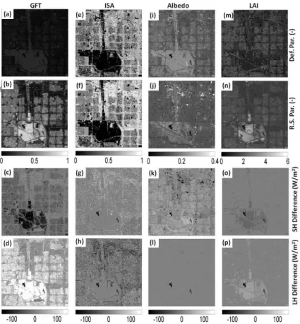
6.2 Spatial evaluation

The spatial distributions of newly assigned GVF, ISA, albedo, and LAI are next com-pared with those based on the Noah-UCM lookup tables. Different urban surface pa-5

rameterizations, along with their impacts on the simulated maps of turbulent sensible and latent heat fluxes, are presented (Fig. 3; Valid at 11:00 LST on 14 April 2011). As expected, during the spring period (April), GVF values are significantly higher when re-mote sensing products are utilized, due to the irrigation effects which are ignored in the default parameters (Fig. 3a and b). Over fully vegetated and low intensity residential 10

pixels, where a significant portion of the energy goes into evaporation and transpira-tion, latent heat flux increases (about 300 and 230 W m−2, respectively) and sensible heat fluxes decreases (about 160 and 120 W m−2, respectively) are found (Fig. 3c and d) when utilizing the remote sensing GVF.

The spatial distributions of ISA, or urban fraction, between the remote sensing and 15

default values show similar patterns (Fig. 3e and f). However, industrial/commercial and high intensity residential areas are assigned noticeably higher urban fraction values in the remote sensing based maps (compare Fig. 3e and f) which leads to lower latent heat fluxes (bias of up to about 130 W m−2) and higher sensible (bias of up to about 10 W m−2) in these pixels (Fig. 3g and h).

20

The Noah-UCM parameters underestimate surface albedo values over highly urban-ized pixels (Fig. 3i and j). In particular, the industrial/commercial buildings with highly reflective rooftops are ignored in the default parameterization. Over the highly veg-etated areas, however, albedo values are overestimated in look-up tables. Altering the energy budget, the newly developed albedo datasets lead to lower Noah-UCM-25

(20)

HESSD

11, 7469–7511, 2014

Title Page

Tables Figures

◭ ◮

Back Close

Full Screen / Esc

Discussion

P

a

per

|

Discus

sion

P

a

per

|

Discussion

P

a

per

|

Discussion

P

a

per

|

over industrial/commercial pixels (up to∼300 W m−2; Fig. 3k). The changes in absolute surface albedos do not affect simulated latent heat fluxes (Fig. 3l).

The remote sensing data detect higher LAI values over all pixel types, particularly over fully vegetated areas where new LAI values are significantly higher (Fig. 3 m and 3n). By influencing the canopy resistance, these changes redefine the spatial distribu-5

tion of turbulent fluxes (Fig. 3o and p). Over the densely vegetated areas, increases in latent heat flux (up to 50 W m−2) and decreases in sensible heat flux (up to 35 W m−2) are found (Fig. 3o and p). It is noteworthy that, as illustrated before (Fig. 3n and o), the most significant influences of LAI alterations are detected in the summer months. Thus, it is not surprising that the turbulent fluxes do not show significant sensitivity to 10

the LAI changes in April.

Remotely sensed emissivity maps, implemented in the Noah-UCM simulations, show minimal effect on the output turbulent fluxes maps (results not shown). Our results (Fig. 2 and 3) agree with previous sensitivity studies performed with the Noah-UCM which indicated high sensitivity of the model to GVF, ISA, albedo, and LAI, and 15

less model sensitivity to emissivity (Loridan et al., 2010; Wang et al., 2011). Loridan et al. (2010) highlighted the critical role of ISA and LAI in the simulations of latent heat flux and albedo role in the sensible heat flux simulations. Investigating the peaks of diurnal turbulent fluxes, Wang et al. (2011) reported that latent heat flux is the most sensitive to the GVF. They also found that emissivity has minimal effects on the model 20

outputs.

7 Evaluation of Noah-UCM performance

After initial sensitivity tests, the model performance in reproducing ET and LST fields is evaluated using remotely sensed (independent from derived parameters) and in situ measurements. The comparisons of observed and simulated ET and LST, using diff er-25

(21)

HESSD

11, 7469–7511, 2014

Title Page

Tables Figures

◭ ◮

Back Close

Full Screen / Esc

Discussion

P

a

per

|

Discus

sion

P

a

per

|

Discussion

P

a

per

|

Discussion

P

a

per

|

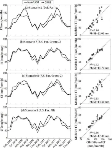
7.1 ET simulations

The temporal variations of ET, simulated by the Noah-UCM model over fully vege-tated pixels, are evaluated against CIMIS-based ET measurements, spanning 2010 and 2011 (Fig. 4). The model reproduces similar ET behaviors when the default param-eters and the second group of remotely sensed paramparam-eters (albedo, LAI, and Emissiv-5

ity) are implemented (Fig. 4a and c). The ET differences between observations and the default simulation are minimal in the winter and fall months, due to the limited energy available for ET in those months. Over the warmer months, the observed and modeled ETs show distinct behaviors. CIMIS stations report two peaks, one in the spring and one in the summer time. Simulated ETs, however, illustrate one peak in the July. The 10

Noah-UCM, using these parameterizations, underestimates ET rates for the most of winter and spring months and overestimates them in the summer time (Fig. 4a and c). Including remotely sensed albedo, LAI, and emissivity does not change the general seasonal pattern deviations of ET (Fig. 4a and c), but it reduces the biases consid-erably (withR2=0.83 and RMSE=14.32 mm month−1). We note that model improve-15

ment is mostly associated with inclusion of remotely-sensed LAI maps in the model since albedo and emissivity have minimal influence on latent heat fluxes from heavily vegetated pixels (see Fig. 2j).

The new GVF and ISA values alter ET seasonal fluctuations significantly in sce-nario 7 (Fig. 4b). In agreement with CIMIS observations, the model with inclusion of 20

remotely sensed parameters results in significantly higher ET values in the warming months (February–May) and lower ETs in the summer time. Noting that ISA has mini-mal effects over the fully vegetated pixels, one explanation for this pattern is that higher green vegetation fraction detected by Landsat in late winter and early spring, increases transpiration rates as soon as the required energy is available and lower measured 25

(22)

HESSD

11, 7469–7511, 2014

Title Page

Tables Figures

◭ ◮

Back Close

Full Screen / Esc

Discussion

P

a

per

|

Discus

sion

P

a

per

|

Discussion

P

a

per

|

Discussion

P

a

per

|

Including all the measured parameter sets (Fig. 4d), reduces the behavioral dis-agreements between observed and modeled monthly ET (R2=0.86). Large biases over the summer months are also reduced. However, ET values are overestimated over the rest of the year (RMSE=17.49 mm month−1). Although each newly developed parameter group enhances the model performance in predicting ET, the advantages 5

are countered when all of the parameters are implemented in the model. This is possi-bly due to the complex interactions between the parameters (e.g., GVF and LAI) in the model structure.

A notable pattern detected by CIMIS data is the drop in ET values over the month of June. The sudden decrease in ET corresponds to the June Gloom weather pattern 10

in southern California, when onshore flows result in persistent overcast skies with cool temperatures, as well as fog and drizzle in late spring and early summer (NWS, 2011). The June Gloom effects are captured in scenarios 7 and 9 (Fig. 4b and d) and not seen in scenarios 1 and 8 (Fig. 4a and c). Since ISA has minimal influence on ET from the fully vegetated pixels and the second group fails to simulate June Gloom influence, the 15

improvements in scenarios 7 and 9, in capturing this phenomenon, are associated with a more accurate representation of GVF.

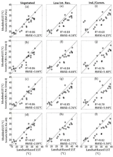
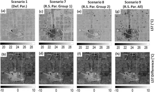
7.2 LST simulations

In order to further evaluate model performance and examine the impacts of diff er-ent remote sensing based parameter sets, Landsat-based LST measuremer-ents are 20

utilized (Figs. 5 and 6). Statistics (R2 and RMSE) are also included to quantify the model performance using different urban surface parameterizations (Fig. 5). The ob-served LSTs, over fully vegetated pixels, are estimated with fair accuracy by the default model (R2=0.86 and RMSE₌3.21◦C; Fig. 5a). The model performance is slightly worse (∼1◦C) over low intensity residential areas (Fig. 5e). Using remote sensing data 25

(23)

HESSD

11, 7469–7511, 2014

Title Page

Tables Figures

◭ ◮

Back Close

Full Screen / Esc

Discussion

P

a

per

|

Discus

sion

P

a

per

|

Discussion

P

a

per

|

Discussion

P

a

per

|

(scenarios 7 and 8) significantly improve the correlations between the observed and simulated LSTs (RMSE of 0.76 and 0.70, respectively; Fig. 5j and k). When all the pa-rameters are used (scenario 9), the RMSE is enhanced to 0.82. However, the cold biases are persistent in all simulations, more significantly over developed surfaces (Fig. 5e–l).

5

Further analysis (not shown here) indicates that underestimation of LST values is due to a fundamental problem in the UCM and cannot be immediately solved with available parameter choices. This problem is discussed in a related study investigating different schemes for LST and conductive heat fluxes in the UCM (Wang et al., 2011b). Their study shows that the current UCM formulation results in a phase lag and cold bi-10

ases in simulated surface temperature when compared to observations. The discussed cold biased could potentially be resolved utilizing a spatially-analytical scheme intro-duced by Wang et al. (2011b).

A comparison of LST at 11:00 LST on 14 April 2011 with four simulation cases is also presented (Fig. 6). Alterations due to use of remote sensing products are more 15

noticeable in this spatial examination of the results. Using all the default parameters (scenario 1), observed LST is overestimated over the heavily vegetated areas and underestimated over highly developed pixels (Fig. 6a and b). Remotely sensed GVF and ISA (in scenario 7) significantly decrease LSTs over fully vegetated and low in-tensity residential pixels and increase temperatures over industrial and commercial 20

areas result in a better match with the observed LST map. However the model still underestimates the observed LSTs over the industrial and commercial pixels (Fig. 6b and e). The decreased simulated surface temperatures over heavily vegetated areas is due to higher GVF and consequently higher ET rates, which in turn lead to lower sensible heat flux and LSTs (see Fig. 3b). The increased LSTs over highly developed 25

(24)

HESSD

11, 7469–7511, 2014

Title Page

Tables Figures

◭ ◮

Back Close

Full Screen / Esc

Discussion

P

a

per

|

Discus

sion

P

a

per

|

Discussion

P

a

per

|

Discussion

P

a

per

|

simulated LSTs over fully vegetated areas are decreased, the observed temperatures are still overestimated (Fig. 6f). The LST decreases in scenario 8 may be explained by evaporative cooling effect of the higher LAI values over heavily vegetated areas (see Fig. 3n). Similar to scenario 7, considerable GVF induced LST reductions, over fully vegetated areas, improve the observed LST estimations in scenario 9 (Fig. 6h). Our 5

assessment indicates that implemented satellite derived parameter maps, particularly GVF and ISA used in scenarios 7 and 9, enhance the Noah-UCM capability to repro-duce the LST differences between fully vegetated pixels and highly developed areas (simulated LST differences of 1.31, 4.81, 1.55, and 4.93◦C for scenarios 1, 7, 8, and 9 vs. observed LST difference of 11.25◦C). Nevertheless, the model still underestimates 10

remotely sensed LST values, by about 9.91◦C for scenario 9, over the highly developed areas.

Regardless of the parameterization processes, cold biases are persistent in all sim-ulations, particularly over high intensity residential and industrial/commercial pixels (Fig. 6). As explained above, this underestimation of LST values is consistent with 15

the literature and is reported to be due to a fundamental problem in the UCM which produces a phase lag and cold biases in simulated LST (Wang et al., 2011b).

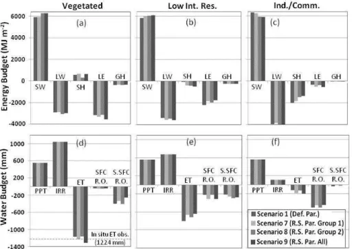
7.3 Energy and water budget evaluation

Differences in the simulated energy and water budgets, with different surface param-eterizations (scenarios 1, 7, 8, and 9 in the Table 1) are summarized for WY 2011 20

(Fig. 7). The emissivity induced changes to the energy and water budgets are insignif-icant and not included. The illustrated radiative and turbulent heat fluxes show that, unlike the longwave radiative fluxes, the simulated available solar radiations are al-tered considerably using di_fferent urban parameter sets (up to 6 %), particularly over fully vegetated (Fig. 7a) and industrial/commercial pixels (Fig. 7c). These changes are 25

(25)

HESSD

11, 7469–7511, 2014

Title Page

Tables Figures

◭ ◮

Back Close

Full Screen / Esc

Discussion

P

a

per

|

Discus

sion

P

a

per

|

Discussion

P

a

per

|

Discussion

P

a

per

|

industrial/commercial areas (Fig. 7c). These turbulent fluxes are also altered when different surface parameterizations are incorporated. Implementing all the remotely sensed parameters (scenario 9), the annual latent heat flux is increased (12 %) over fully vegetated pixels (Fig. 7a), and the annual sensible heat flux is decreased (32 %) over industrial/commercial pixels (Fig. 7c). Ground heat fluxes, however, are insignifi-5

cant and unchanged.

Water budget terms also show variable behavior using different parameter sets over different land cover types (Fig. 7d–f). Annual irrigation amounts exceed received pre-cipitations over the pixels with significant vegetation fractions (Fig. 7d and e). This pattern is not rare in semi-arid regions (CDWR, 1975; Mini et al., 2014). In these areas, 10

most of incoming water is lost through ET (Fig. 7d and e). Areas with high coverage of impervious surfaces, however, dissipate most of the incoming moisture through sur-face runoff(Fig. 7f). The alterations in the annual ET rates are, for the most part, due to the changes in the GVF parameterizations (scenarios 7 and 9; Fig. 7d–f). Sub-surface runoffannual rates, on the other hand, are altered using new ISA values (scenarios 7 15

and 9; Fig. 7e and f). Changes in the annual ET values are as large as 145, 156, and 79.4 mm over fully vegetated, low intensity residential and industrial/commercial pixels, respectively (Fig. 7d–f).

To further verify the capability of Noah-UCM to reproduce observed ET quantities, additional evaluation of the model is conducted utilizing ground-based chamber ET 20

measurements in the greater Los Angeles area (Moering, 2011). Instantaneous ET measurements, over an irrigated park in the study domain during WY 2011, are con-verted to daily and then annual ET estimates (1224 mm) and compared with the simu-lated ET values over the parks (Fig. 7d). As expected, the observed ET is best repro-duced by scenario 7 (Bias of 1.47 mm) due to more accurate representation of GVF in 25

(26)

HESSD

11, 7469–7511, 2014

Title Page

Tables Figures

◭ ◮

Back Close

Full Screen / Esc

Discussion

P

a

per

|

Discus

sion

P

a

per

|

Discussion

P

a

per

|

Discussion

P

a

per

|

sets, used in scenarios 1 and 8, (2) the uncertainties associated with the estimated LAI values utilized in scenarios 8 and 9, and (3) complex interactions between GVF and LAI noted in scenario 9.

The presented analysis of energy balance (Fig. 7) suggests that GVF, albedo and LAI play an important role in regulating simulated radiative energy budget and turbulent 5

fluxes, mainly by affecting the available net radiation and transpiration quantities. GVF, ISA, and LAI also alter the study area transpiration and ET values, as well as surface runoffrates.

8 Conclusions

In the current work we investigate the utility of a select set of remote sensing based 10

surface parameters in the Noah-UCM modeling framework over a highly developed ur-ban area. It was found that remote sensing data show significantly different magnitudes and seasonal patterns of GVF when compared with the default values. The reason for this mismatch is the significant and year round irrigation in the Los Angeles area which is not accounted for in the default parameter tables. Irrigated landscapes maintain con-15

stant greenness rather than a seasonal behavior of greening in the winter/spring and browning in the summer. The noticed differences between the monthly LAI values from default tables and remotely sensed data are also due to complex irrigation patterns. Another factor that contributes to this mismatch is the fact that landscape plantings are quite different from agricultural crops due to their being composed of collections of 20

vegetation species which is not taken into account in the vegetation parameter tables in the Noah LSM (CDWR, 2000; Vahmani and Hogue, 2013, 2014). There are also considerable deviations between the look-up-table ISA, albedo and emissivity maps and the remotely sensed values. The results of our analysis agree with previous stud-ies which show high sensitivity of the Noah-UCM to GVF, ISA, albedo, and LAI, and 25

(27)

HESSD

11, 7469–7511, 2014

Title Page

Tables Figures

◭ ◮

Back Close

Full Screen / Esc

Discussion

P

a

per

|

Discus

sion

P

a

per

|

Discussion

P

a

per

|

Discussion

P

a

per

|

results show that GVF, ISA and LAI are critical in the simulations of latent and sensible heat flux, and that albedo plays a key role in the sensible heat flux simulations.

Our assessment of the Noah-UCM ET estimation shows that using the default pa-rameters leads to significant errors in the model predictions of monthly ET fields (RMSE=22.06 mm month−1) over the study domain in Los Angeles. Results show 5

that accurate representation of GVF is critical to reproduce observed ET patterns over vegetated areas in the urban domains. LAI also plays an important role in ET simulations. However, simulations incorporating the remotely sensed GVF val-ues outperform (RMSE=11.77 mm month−1) simulations with the new LAI estimates (RMSE=14.32 mm month−1). This could be due to several reasons. First, there are 10

uncertainties associated with the remote sensing based LAI retrieval, including non-linearity of LAI-vegetation index (RSR) relationships (Latifi and Galos, 2010), which do not apply to NDVI-based GVF. Second, more accurate representation of GVF values in the Noah-UCM not only improves the assigned LAI values to the vegetated pixels in the model but also enhances other parameters inputs as well (i.e., albedo, emissivity, 15

and roughness length). Further analysis of the model performance indicates that im-plemented satellite derived parameter maps, particularly GVF and ISA, enhance the Noah-UCM capability to reproduce the LST differences between fully vegetated pixels and highly developed areas (simulated LST differences of 1.31 and 4.81◦C for sce-narios with default and remotely sensed GVF and ISA vs. observed LST di_fference of 20

11.25◦C). Nevertheless, the model still underestimates remotely sensed LST values, over highly developed areas. We speculate that the underestimation of LST values, particularly over high intensity residential and industrial/commercial areas, is due to structural parameterization in the UCM and cannot be immediately solved with avail-able parameter choices.

25

(28)

HESSD

11, 7469–7511, 2014

Title Page

Tables Figures

◭ ◮

Back Close

Full Screen / Esc

Discussion

P

a

per

|

Discus

sion

P

a

per

|

Discussion

P

a

per

|

Discussion

P

a

per

|

and surface runoff. When compared with in-situ observations, Noah-UCM shows the capacity to reproduce ET fields with relatively high accuracy (Bias of 1.47 mm) when GVF maps are updated using remote sensing data.

In summary, the current study highlights the significant deviations between the spa-tial distributions and seasonal fluctuations of the default and remotely sensed param-5

eter sets in the Noah-UCM. We illustrate that replacing default parameters with the measured values reduces significant biases in model predictions of the surface fluxes within irrigated urban areas. This ultimately has key implications in feedback processes to the atmosphere when the Noah-UCM is coupled with the widely used WRF model, which has been increasingly applied over urban areas to examine the exchange of 10

heat, moisture, momentum or pollutants. Semi-arid urban cities are receiving much at-tention in the literature, given their accelerated growth and increasing dependence on external water sources. More accurate representation of both water and energy fluxes is critical for regional resource management as well as predictions of urban processes under future climate conditions.

15

Acknowledgements. Funding for this research was supported by an NSF Hydrologic Sci-ences Program CAREER Grant (#EAR0846662), a 2012 NASA Earth and Space Science Fellowship (#NNX12AN63H), and an NSF Water Sustainability and Climate (WSC) grant (#EAR12040235).

References

20

Arnfield, A. J.: Two decades of urban climate research: a review of turbulence, exchanges of energy and water, and the urban heat island, Int. J. Climatol., 23, 1–26, doi:10.1002/joc.859, 2003.

Artis, D. A. and Carnahan, W. H.: Survey of emissivity variability in thermography of urban areas, Remote Sens. Environ., 12, 313–329, 1982.

25