www.ann-geophys.net/27/4409/2009/
© Author(s) 2009. This work is distributed under the Creative Commons Attribution 3.0 License.
Annales
Geophysicae
Determination of the electron temperature in the modified
ionosphere over HAARP using the HF pumped Stimulated Brillouin
Scatter (SBS) emission lines
P. A. Bernhardt1, C. A. Selcher1, R. H. Lehmberg1, S. Rodriguez2, J. Thomason2, M. McCarrick3, and G. Frazer4
1Plasma Physics Division, Naval Research Laboratory, Washington, D.C. 20375, USA 2Radar Division, Naval Research Laboratory, Washington, D.C. 20375, USA
3BAE Systems, Washington, D.C., USA 4ISR Division, DSTO, Edinburgh, SA, Australia
Received: 20 April 2009 – Revised: 23 August 2009 – Accepted: 17 September 2009 – Published: 4 December 2009
Abstract. An ordinary mode electromagnetic wave can de-cay into an ion acoustic wave and a scattered electromagnetic wave by a process called stimulated Brillouin scatter (SBS). The first detection of this process during ionospheric modi-fication with high power radio waves was reported by Norin et al. (2009) using the HAARP transmitter in Alaska. Sub-sequent experiments have provided additional verification of this process and quantitative interpretation of the scattered wave frequency offsets to yield measurements of the elec-tron temperatures in the heated ionosphere. Using the SBS technique, electron temperatures between 3000 and 4000 K were measured over the HAARP facility. The matching con-ditions for decay of the high frequency pump wave show that in addition to the production of an ion-acoustic wave, an electrostatic ion cyclotron wave may also be produced by the generalized SBS processes. Based on the matching condition theory, the first profiles of the scattered wave am-plitude are produced using the stimulated Brillouin scatter (SBS) matching conditions. These profiles are consistent with maximum ionospheric interactions at the upper-hybrid resonance height and at a region just below the plasma res-onance altitude where the pump wave electric fields reach their maximum values.
Keywords. Electromagnetics (Wave propagation) – Iono-sphere (Active experiments) – Radio science (Waves in plasma)
Correspondence to:P. A. Bernhardt ([email protected])
1 Introduction
Many types of waves exist in the ionospheric F-region plasma that is primarily composed of electrons and O+ ions in the earth’s magnetic field. The waves supported in this plasma include O-mode and X-mode electromagnetic waves, electron plasma waves, ion acoustic waves, upper hy-brid waves, lower hyhy-brid waves, electron and ion Bernstein waves, electron whistler waves, and ion cyclotron waves. A high power electromagnetic wave from a ground transmitter can act as a pump to excite a pair of growing waves through the parametric decay instability. An overview of both ob-servations and theory of parametric decay processes in the ionosphere pumped by high power EM waves is given by the detailed monograph on stimulated electromagnetic emis-sions (SEE) by Leyser (2001). Parametric decay processes that have been postulated to occur in the magnetized iono-sphere include the decay of the O-mode EM wave into (a) an ion acoustic and an electron plasma wave, (b) a lower hybrid and upper hybrid wave, and (c) a lower hybrid and electron Bernstein wave.
With the recent upgrade of the High Frequency Active Auroral Research Program (HAARP) facility in Alaska, it is likely that some new parametric instability will be de-tected in the ionospheric interactions processes. The HAARP ionospheric modification system is comprised of 180 crossed dipoles in a 12×15 array. Each dipole is fed by a separate 10 kW transmitter that allows separate excitation of the phase and amplitude. With all transmitters operating simultane-ously, a total of 3.6 MW power can be supplied to the antenna array. The effective radiated power (ERP or the product of transmitter power and antenna gain) for the array varies with frequency. The results reported here are for operation at 4.5 and 5.6 MHz with effective radiated powers greater than 1 gigawatt. The HAARP beam was phased for O-Mode left-circular polarization to allow propagation of the HF wave for interactions near the critical layer where the wave frequency is equal to the local plasma frequency.
In a recent paper, Norin et al. (2009) have produced the first detection in the ionosphere of an electromagnetic pump from the ground exciting the stimulated Brillouin scatter (SBS) instability using transmissions from the HAARP fa-cility in Alaska. They recorded the stimulated electromag-netic emissions (SEE) in a 100 Hz band near the pump fre-quency. The emissions that occurred near±9 Hz of the pump frequency were attributed to interactions near the HF wave reflection altitude where the wave frequency is equal to the local value of plasma frequency. Another set of emissions near±25 Hz were attributed to interactions near the upper hybrid resonance altitude where the pump frequency equals the local upper hybrid frequency.
Norin et al. (2009) successfully argue that the recorded scattered EM waves arise from process (2) for the laser plasma interactions where an electromagnetic wave decays into an ion acoustic wave and a scattered electromagnetic wave. In the SBS process, density fluctuations associated with ion acoustic waves couple with the pump electromag-netic wave to produce the scattered electromagelectromag-netic wave. This scattered EM wave may in turn couple with the pump wave to reinforce the ion acoustic wave. These couplings can lead to the growth of scattered electromagnetic waves along with ion acoustic waves giving the Brillouin instability (Kruer, 1988; Eliezer, 2002).
Stimulated Brillouin scattering can be inhibited by both collisional and Landau damping in the ionosphere. Sev-eral factors favor the production of SBS in the ionosphere. The electron-neutral collision frequency in the ionosphere is relatively low during the current period of solar minimum because of low atmospheric neutral densities. Second, the HAARP facility has been recently upgraded to a 12×15 an-tenna array with a total of 3.6 megaWatt power feeding this array. With more power, the HF beam will provide an electric field that can more often exceed the threshold for SBS and also produce larger increases in electron temperature. Higher electron temperatures are also found when heating plasmas of lower density because of reduced cooling of the
trons onto the ions (Djuth et al., 1987). The elevated elec-tron temperatures during ionospheric heating greatly reduce both electron-ion collision frequencies and Landau damping of ion acoustic waves.
The primary purpose of this paper is to extend the work of Norin et al. (2009) by developing a quantitative theory of SBS in a magneto-plasma like the ionosphere. The wave number and wave frequency matching conditions are solved with the dispersion equations for the ion acoustic and elec-tromagnetic waves keeping all of the effects of the ion and electron gyro frequencies. These solutions provide an ana-lytic expression that will yield measurements of the electron temperatures in the upper hybrid interaction regions based on the frequencies of the widely spaced SBS lines.
This paper also presents new measurements of the SBS lines for frequencies or conditions not explored in the previ-ous work by Norin et al. (2009). With both increased power for electromagnetic pump at HAARP and low neutral den-sities in the upper atmosphere, the conditions are ideal for experimental studies of SBS. On 24 October 2008, a digi-tal receiver called the GBOX5 developed at DSTO in Aus-tralia was operated near the HAARP transmitter to detect stimulated electromagnetic emissions (SEE). The results of the experiment, given in the next section, show that SBS produces an SEE spectrum of electromagnetic waves with spectral lines that are offset from the pump frequency by the ion-acoustic frequency in the plasma. This interpretation is validated in Sect. 3 by a theoretical derivation of the wave matching conditions for producing SBS in magnetized plas-mas like the ionosphere. The electric field amplitudes of the pump wave and the location of the upper-hybrid resonance region in the ionosphere are described in Sect. 4.
With the SBS matching conditions, the measured electro-magnetic spectra are mapped to the plasma densities in the ionosphere. For vertical HF beams, the measured SBS emis-sions are shown to be consistent with electromagnetic waves at the region where the pump frequency is equal to the upper-hybrid frequency. The matching conditions are applied to give a relation between the electron temperature and the SBS emission spectra. With this relation, the electron temperature in the modified ionosphere can be measured using the ion-acoustic wave shifts in the SEE data along with knowledge of the electron and ion cyclotron frequencies at the ionospheric interaction heights. Thus the stimulated Brillouin spectra in-terpretation provides a powerful remote sensing tool for the modified ionospheric environment.
2 Experimental measurements of Stimulated Brillouin Scatter using HAARP
the waves was captured with a digital receiver called the GBOX5 using digital sampling and continuous recording of a ±125 kHz around the HF pump frequency. For the measure-ment of the stimulated electromagnetic emissions (SEE), an initial data sample time of 4 microseconds was used. Suc-cessive 600 points are averaged to provide data with a 2.4 ms sample period for the low-frequency spectral analysis. The stored in-phase and quadrature-phase (I and Q) data samples were processed to yield spectra of the backscatter wave side-bands around the pump wave center frequency with a resolu-tion of 1.39 Hz. The SEE spectrum is displayed in dB power relative to the maximum input power that will saturate the GBOX5 receiver. The input attenuation to the receiver was adjusted to prevent this saturation by the pump wave reflected from the ionosphere.
The GBOX5 recording system was located 20 km from the HAARP transmitter using a vertical pointing inverted V antenna with the nomenclature AS-2259/GR. This antenna is used as a near vertical incidence skywave antenna in the 3.5 to 10 MHz frequency range. This lightweight, sloping dipole, omnidirectional antenna is ideal for SEE measure-ments because of its frequency range and portability. The same antenna was used for the SEE measurements of Norin et al. (2009).
The HAARP transmitter frequency was fixed at 4.5 MHz in the time period between 19:40 to 20:00 UT (11:40 to 12:00 Local Time) on 24 October 2008. The 4.5 MHz HF trans-missions from HAARP ware generated in 120 s periods with 90 s on and 30 s off. The transmitter was either operated in a standard beam with all antenna elements in phase or in an orbital angular momentum configuration (OAM) with the an-tenna elements phase equal to their azimuthal position rela-tive to the center of the array (Leyser et al., 2009). The OAM configuration produces a wider beam with a null along the beam axis. The GBOX5 receiver recorded data continuously through this transmission period.
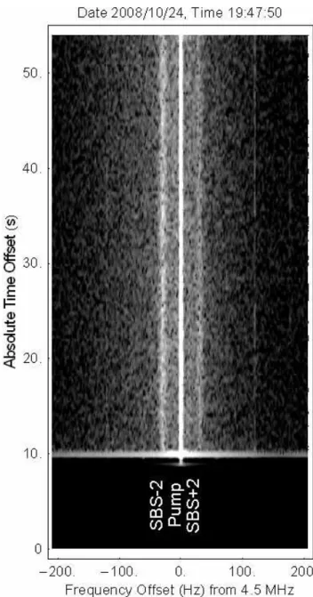
A spectrogram of the recorded SEE was produced from successive 0.8 s data samples. The dynamic spectra recorded for a full power (1 GW ERP) vertical-beam transmission at 4.5 MHz is illustrated in Fig. 1. After a transient produced by the HAARP transmitter at turn on, the SEE spectra shows the central pump line, two stimulated Brillouin scatter lines around the pump and narrow lines at 120 and 180 Hz. These latter features along with 60 Hz lines reported by Norin et al. (2009) are the result of the 60 Hz harmonics in the power supplies for the transmitter. The SBS lines were imbedded in a low-frequency continuum emission that may be produced as spectral noise by the HAARP transmitter. The HAARP transmitter transient that is shown as an initial broadening of the spectra in Fig. 1 has been reduced for future experiments. The frequencies of the labeled lines in Fig. 2 were ob-tained by averaging the 90 s of spectral data. Each individual spectrum was obtained with a Blackman window of the data. The 120 Hz lines, produced by power supply ripple in the HAARP transmitter, are used to verify the frequency
cali-Fig. 1.Time history of the SEE spectra near the HF pump frequency of 4.5 MHz. The data were obtained on 24 October 2008 when the HF wave was turned on at 19:48 UT. The wave induced stimulated Brillouin scatter (SBS) lines near 30 Hz are broader than the artifi-cial power line harmonics at 120 and 180 Hz.
Fig. 2.Spectra of scattered electromagnetic waves from the HAARP transmitter operating at 4.5 MHz with 1 GW effective radiated power. All the data were taken within a 20 min period on 24 October 2008. The downshifted lines are also called the Stokes lines, downshifted SBS- lines or the downshifted narrow peaks (np-). The upshifted lines are similarly called the anti-Stokes lines, upshifted SBS+ lines or the upshifted narrow peaks (np+). The 120 Hz lines are produced by power ripple in the transmitter power system.
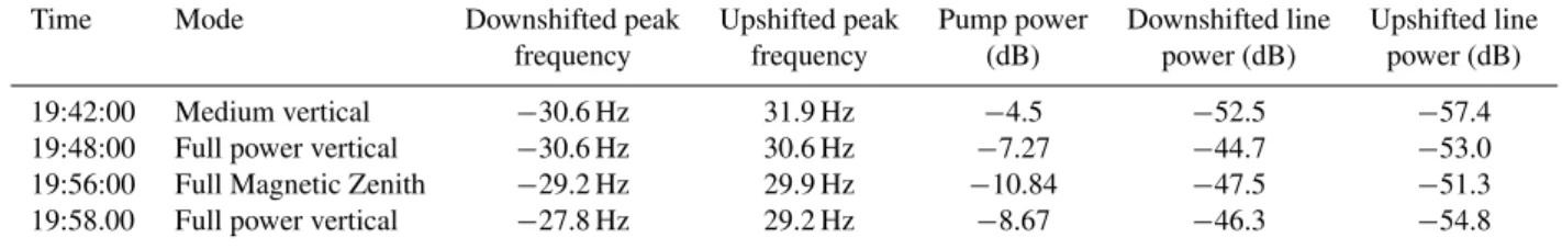
Table 1.SBS scattered electromagnetic line strengths and frequencies for a 4.5 MHz pump wave.
Time Mode Downshifted peak Upshifted peak Pump power Downshifted line Upshifted line frequency frequency (dB) power (dB) power (dB) 19:42:00 Medium vertical −30.6 Hz 31.9 Hz −4.5 −52.5 −57.4 19:48:00 Full power vertical −30.6 Hz 30.6 Hz −7.27 −44.7 −53.0 19:56:00 Full Magnetic Zenith −29.2 Hz 29.9 Hz −10.84 −47.5 −51.3 19:58.00 Full power vertical −27.8 Hz 29.2 Hz −8.67 −46.3 −54.8
Indeed, all of the SBS lines presented by Norin et al. (2009) also had stronger down shifted lines than the up-shifted (anti-Stokes) lines. Norin et al. (2009) has similar displays of±30 Hz lines for vertical beams of HAARP HF waves. When the HF beam was pointed toward the magnetic zenith, however, the SBS spectra showed two sets of lines. One set was near±30 Hz as illustrated in Fig. 2c but in the same spectra there was a second set of lines near ±15 Hz when the HF beam was aligned with the magnetic field lines. None of the measurements made at 4.5 MHz showed this ef-fect.
The stimulated Brillouin scatter (SBS) lines were observed using (1) a vertical HF beam in an orbital angular momen-tum (OAM) or twisted beam configuration with a
transmit-ter power of 1.86 MW (Fig. 2a), (2) full standard beam with 3.6 MW transmitter (Fig. 2b and d), as well as (2) a magnetic aligned standard beam with 3.6 MW transmitter (Fig. 2c). All of the SBS lines were located very close to±30 Hz from the pump wave. The line frequency offsets shown in Fig. 2 are found as an average of the full 90 s when the HF was operating.
difference for excitation of SBS with the OAM beam or with a more-standard circularly polarized pump without orbital-angular-momentum. This study will be presented in a future paper.
The locations of the SBS lines were not significantly af-fected by either the shape and power of the pump wave or the tilting of the beam to the vertical or the magnetic zenith. Fig-ure 2 is the first display of SBS lines at the same frequency, with a variety of beam configurations, and with a very short time period between each measurement. We find that tilting the HF beam or changing the beam shape has no measurable affect on the frequencies of the SBS lines relative to the fixed 4.5 MHz pump wave.
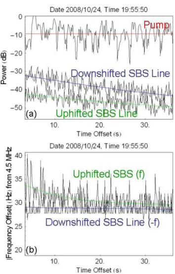
The Stokes (SBS-) and anti-Stokes (SBS+) lines are not exactly the same offset from the pump frequency. This low frequency offset near 30 Hz varies with time. The systematic variation is illustrated in Fig. 3 with the beam pointed toward the magnetic zenith. When the transmitter is turned on, the pump echo at 4.5 MHz shows large fluctuations around an average of about−10 dB on our relative scale. With the same scale, the power in the upshifted and downs shifted lines both decay by about 9 dB over a period of 30 s.
The magnitude of the frequency shifts for the SBS lines relative to the pump are not the same when the data is exam-ined in detail. The offset magnitude of the upshifted line is about 1 Hz or larger than the frequency offset for the down-shifted line. As illustrated in Fig. 3, absolute value of the fre-quency offset for the upshifted line asymptotically changes with time reaching an equilibrium value in about 20 s. This indicates that the SBS interactions in the plasma have slightly different conditions for the Stokes and anti-Stokes lines and these conditions for the weaker upshifted line are changing. This shift in the upshifted frequency offset probably results from Doppler shifts of the ionospheric reflected HF wave that scatters with ion-acoustic waves to produce the weaker up-shifted, anti-Stokes line (see Sect. 4.). The frequency of the downshifted line does not change with time because the SBS occurs before reflection occurs.
For comparison, another sample of the SEE showing SBS lines is shown in Fig. 4. The SBS measurements at 5.6 MHz used a 10-min long continuous wave transmission toward the magnetic zenith. The spectrum is dominated by a large downshifted line labeled SBS-1 located 16.7 Hz below the electromagnetic pump frequency. Two weak lines called SBS+1 at 16.7 Hz and SBS+2 at 34.7 Hz are found above the pump frequency. From the data, it is not clear if the SBS+2 line is a cascade of SBS+1 or a separate emission line. Norin et al. (2009) interpret the low frequency lines (SBS±1) as originating near the reflection altitude and the UH resonance altitude as the source for the (SBS+2). All of the magnetic zenith SBS spectra provided by Norin et al. (2009) showed the strong downshifted lines near 17 Hz.
The purpose of this paper is to provide a quantitative in-terpretation of the SBS spectra to measure (1) the electron temperatures in the heated plasma and (2) the profile of the
Fig. 3. Temporal variations in the(a)powers and(b)frequencies of the SBS line features. The average pump power stays nearly constant while the powers of both the upshifted and downshifted lines drop with time. The frequency of the pump remains fixed, but the offset of the upshifted SBS line drops from 34 Hz to about 30 Hz in 30 s. The downshifted SBS line remains at about 29 Hz frequency.
scattered electromagnetic waves near both the reflection and the upper-hybrid resonance regions. For this interpretation, detailed knowledge of the background ionosphere, ambient electric field, and collisional absorption is required. Mea-surement of the ambient environment is discussed in the next section.
3 Background environment during the SBS measurements
Fig. 4.Stimulated electromagnetic emission spectra for a 5.6 MHz pump wave pointed toward the magnetic zenith from HAARP. A down shifted SBS-2 line may be masked by the low-frequency side of the strong SBS-1 line.
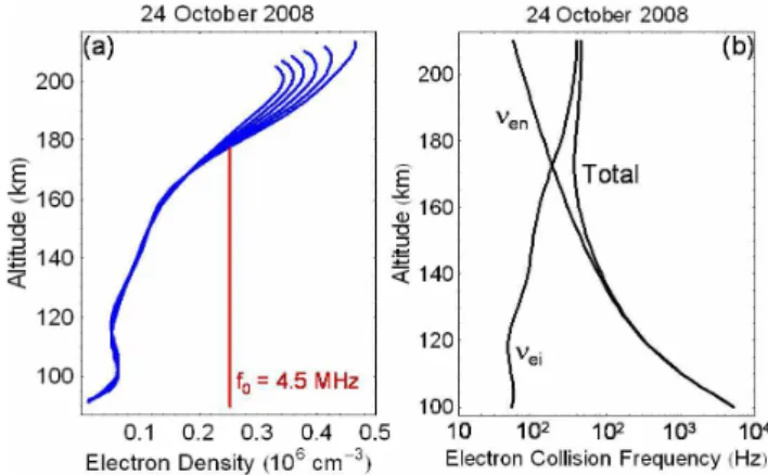
at 19:35 and 20:00 UT on 24 October 2004 were analyzed to provide true height profiles of the bottomside ionosphere. Linear interpolation of the ionogram data was used to pro-vide the family of profiles illustrated in Fig. 5a. The plasma layers are stable below 170 km altitude over the 25 min of the ionosonde measurement. Above 170 km, the F-layer densi-ties are increasing causing a small amount of increase in the bottom side gradients between 170 and 190 km altitude. The ionogram data indicates that the F-region ionosphere was sta-ble between 19:40 UT and 20:00 UT during the time of the high power radio wave experiments. The accurate electron density profile is essential to aid the determination of the al-titude of the HF interactions in the plasma.
The magnetic field in the ionosphere is needed to de-termine the wave propagation characteristics of the mag-netized plasma. The International Geomagnetic Reference Field (IGRF) model provided the magnetic field strength and direction in the upper atmosphere over HAARP. The mag-netic field near the HF reflection altitude is estimated to be |B|=5.205×10⁻⁵Tesla with a dip angle of 75.5 degrees.
The electron-ion and electron-neutral collision frequencies can affect the amplitude of the electromagnetic pump wave. The electron-ion collision frequency is calculated from the ion densities using the standard formula from Goldston and Rutherford (1995)
νei=
√
2nie4ln3
12π3/2ε2 0
√m
eTe3/2
(1)
whereniis the ion density (equal to the electron density from
the ionosonde),Teis the electron temperature in energy units
(Joules) and ln3=14 in the ionosphere.
The NRL-MSIS00 model was used to estimate the neutral densities in the upper atmosphere over the HAARP
transmit-Fig. 5. Altitude profiles for(a)measured electron density profiles and(b)estimated electron-neutral (νen)and electron ion (νei)
col-lision frequencies for the period of the ionospheric modification experiments. Ionograms taken at 19:35 and 20:00 UT were ana-lyzed and interpolated to provide the electron density profiles and electron-ion collision frequencies. The NRL-MSIS00 model pro-vided the neutral densities for the estimates ofνen.
ter. These densities are converted into electron-neutral colli-sion frequencies by the formula from Yeh and Liu (1972) νen=8.88×10⁻⁵
p
Te(nO2+nN2+2nO) (2) where Te is the electron temperature (again in Joules),
nO2,nN2 andnOare the molecular oxygen, molecular nitro-gen, and atomic oxygen densities in m−3, respectively and νenis in s−1. The electron-neutral collision frequencies
dur-ing the October Period of 2008 (Fig. 5b) are very low be-cause of low neutral densities during the current solar mini-mum period. Near the reflection altitude, estimated value of νen is 128 s−1andνeiis 222 s−1giving a total electron
col-lision frequency ofνeT=350 s−1. In addition, D-region
ab-sorption by electron neutral collisions during the daytime or during times of strong electron precipitation can significantly reduce the intensity of the pump wave before it interacts in the F-layer.
The next step is to derive a theory for stimulated Bril-louin scatter (SBS) in a magnetized plasma. Previous work on SBS dealt with laser-plasma interactions where the back-ground magnetic field plays an insignificant role in the SBS process. The basis for SBS is the parametric decay of an electromagnetic pump wave into an ion acoustic wave and a backscattered EM wave. The ionosphere has a strong enough magnetic field to affect the propagation of both electromag-netic and the ion-acoustic waves. The matching conditions for production of SBS are derived in the next section.
4 Wave matching conditions for Stimulated Brillouin Scatter in magnetized plasmas
Brillouin Scatter (SBS) (Norin et al., 2009). The up-going electromagnetic pump wave at ω0 decays into (1) a high-frequency, down-going scattered electromagnetic wave atωS
and (2) a low-frequency wave at frequencyωL. The wave
frequency and wave propagation direction are given by the energy and momentum conservation equations
ω0=ωS+ωL
k0=kS+kL (3)
wherek0,kS, andkLare the wave numbers for the upward
electromagnetic pump, scattered electromagnetic wave and ion-acoustic wave, respectively (Kruer, 1988; Eliezer, 2002). This indicates that a photon or electromagnetic wave of one energy or frequency cannot produce a decay product with higher energy or frequency. Also the directional momentum of the decay products is conserved so that the decay prod-ucts of an upward propagating wave must have at least one upward component.
Low frequency electrostatic waves are described by the dispersion equation for plasma waves as given by Eq. (4.20.3) of Yeh and Liu (1972).
1− Xe(1−Y 2
eCos2θ )
1−Ye2−n2Lδe(1−Ye2Cos2θ )
− Xi(1−Y 2
iCos2θ )
1−Yi2−n2Lδi(1−Yi2Cos2θ )
=0 (4)
where the magneto-ionic parameters of normalized electron density, normalized gyro frequency, normalized thermal ve-locity, and refractive index are respectively defined as
Xe,i=
ω2pe,i ω2L =
Ne,ie2
me,iε0ω2L
,Ye,i=
e,i
ωL
= meB
e,iωL
,δe,i=
v2T e,i c2 =
γe,iTe,i
me,ic2
,nL=
kLc
ωL
. (5) and Te,i are the electron and ion temperatures in energy
units. The angle θ is between the wave normal direction and the background magnetic field vector and it satisfies
B·kL=|B||kL|Cosθ. For vertical propagation of both ion
acoustic and electromagnetic waves through a horizontally stratified medium,θis fixed at the complement of the mag-netic dip angle over HAARP.
The ionosphere is assumed to be composed of positively charged oxygen ions with massmi and electrons with mass
me with me≪mi. Also, the ion sound waves have
wave-lengths much larger than a Debye length sokLλD≪1 where
the Debye length isλD=
qγ
eTeε0
Nee2 . Under these conditions,
Eq. (4) simplifies to
ω4L−(2i+k2Lc2IA)ωL2+2ikL2c2IACos2θ=0 (6) wherecIA=
q
γeTe+γiTi
mi is the ion acoustic velocity withγe=1
andγi=3 (Stix, 1992). The solution of Eq. (6) forkLhas a
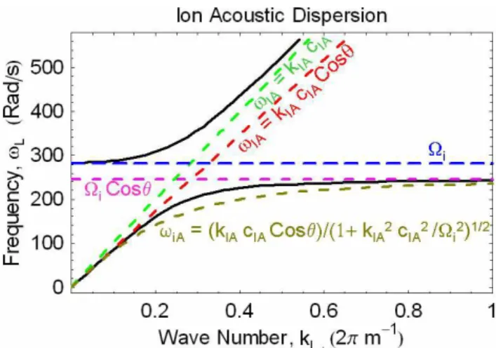
Fig. 6.Zeros, poles and limiting forms for the ion acoustic disper-sion Eq. (6) near the ion gyro frequency. The black curve repre-sents the most exact form used to compute the SBS matching con-ditions. Ion acoustic wave are found for frequencies belowiCosθ whereθis the wave normal angle relative to the magnetic field di-rection. Electrostatic ion cyclotron wave are found for frequencies just above thei.
zero atωL=i and a pole atωL=iCosθ. This dispersion
equation is illustrated in Fig. 6.
Two solutions to Eq. (6) are found forω2L assuming that |kL cIA<|i|. For frequencies abovei, the electrostatic
ion cyclotron (EIC) wave (Stix, 1992) is found with the fre-quency determined from
ω2EIC=
2i+kEIC2 c2IA+ q
(2i−kEIC2 c2IA)2+4k2
EICc2IA2iSin2θ
2 ∼
=2i+ k 2
EICc2IASin2θ
1−kEIC2 c2IA/ 2i ifk 2
EICc2IA≪2i (7)
The second low-frequency mode is the ion acoustic (IA) wave with the negative sign before the radical
ω2IA=
2i+k2IAc2IA− q
(2i+k2IAcIA2 )2−4k2
IAcIA2 2iCos2θ
2 (8)
To second order in|kIAcIA|/|i|, the ion acoustic wave
dis-persion is given as ω2IA=k
2
IAc2IA2iCos2θ
(2i+kIA2 c2IA) (9) This equation was used by Norin et al. (2009).
For ion acoustic frequencies much larger than the ion cy-clotron frequency (i.e.,ωIA≫2ci), Eq. (6) becomes
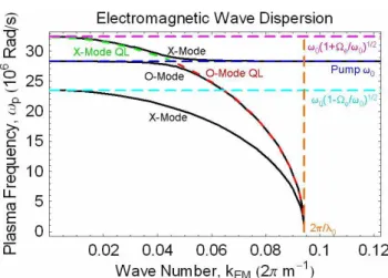
Fig. 7. Ionospheric plasma frequency for a 4.5 MHz electromag-netic wave with a range of wave numbers extending past the free-space wave number.
acoustic wave for either a pump wave that is much larger than the plasma frequency (Fejer, 1979) or a plasma with zero magnetic field (Kruer, 1988).
Since neither Eq. (9) nor Eq. (10) are valid for low-frequency modes near the ion gyro low-frequency, they will not be used here. The full dispersion Eq. (6) will be employed to determine the SBS matching conditions. Both ion acous-tic waves and electrostaacous-tic ion-cyclotron waves are included in this dispersion equation. The full dispersion equation along with the approximate forms are illustrated by Fig. 6 forcIA=1000 m/s,θ=15◦, andi=283 rad/s (45 Hz).
SBS involves two electromagnetic waves, one pump wave with subscript “0” and one scattered wave with subscript “s”, that satisfy the Appleton-Hartree (A-H) equation. These waves can have O-Mode or X-Mode polarization as indicated by superscript “O” or “X”, respectively. With Cartesian co-ordinates defined by Yeh and Liu (1972) such that the prop-agation vector is in the z-direction and the magnetic field vector is in the yz-plane, the transverse polarization is de-fined asR(z)=Ex/Ey=−Hy/Hx for the transverse fields of
each mode. The refractive index for these modes is given by Eq. (4.14.19) by Yeh and Liu (1972)
n(O,X)= s
1− X
U+iY RO,XCosθ
(11)
wheren(O,X)=k(O,X)c/ωis the O-Mode and X-Mode refrac-tive index,R(O,X)is the wave polarization given by
R(O,X)(z)= i Cosθ
YSin2θ 2(U−X)∓
s
Y2Sin4θ 4(U−X)2+Cos
2θ
,(12)
the magnetoionic parameter definitions similar to those given in Eq. (5) with electromagnetic frequencyωandU=1−iνen
ω
represents collisional loss between electrons and ions at rate
νen. In terms of frequencies and wave numbers the
electro-magnetic wave dispersion equationk2c2=n2ω2 for electro-magnetic propagation in a magneto-ionic plasma is
2(ω20,S−ωp2)ω2p ω20,S−k02,Sc2 =
2(ω20,s−ω2p)−2eSin2θ (13)
± v u u t
4(ω20,S−ω2
p)22eCos2θ
ω20,S + 4
eSin4θ
where the form is chosen so the + sign is used for the ordi-nary (O-Mode) propagation and the−sign for the extraor-dinary (X-Mode) propagation and the collisional loss term has been neglected. The low collision frequencies (Fig. 5b) have a negligible effect on the matching conditions but they will be re-introduced with computations of the amplitudes for the high power pump wave in the next section. For propaga-tion approximately alongBwithθ≪1, the quasi-longitudinal (QL) approximation of Eq. (13) is given by
ω2p=ω02,S−k20,Sc2
1±Sign[ω0,S−ωp]
eCosθ
ω0,S
(14) but this equation is only valid if
Cos2θ≫ ω 2
0,S2eSin4θ
4(ω2
p−ω20,S)2
. (15)
Near the plasma resonance region where the plasma fre-quency is close to the wave frefre-quency the condition in Eq. (15) will break down. The relationship between the ionospheric plasma frequency and the electromagnetic wave number for propagation atω0=4.5 MHz is shown in Fig. 7. The magneto-ion conditions are the same as for Fig. 6. The QL solutions are given by the red and green curves, respec-tively, for O-mode and X-mode propagation.
Since the SBS is expected to occur near to where the elec-tromagnetic wave amplitude swells to a maximum at the crit-ical layer near whereωp∼ω0,S, the complete A-H
formula-tion (Eq. 13) will be used for the full theoretical descripformula-tion. As illustrated in Fig. 7, the only mode that will propagate from the ground to the resonance region is the O-mode so the + sign in Eq. (13) is the most relevant to the model of the SBS matching conditions. The X-mode with the−sign in Eq. (13) also will be considered in the analysis for complete-ness because if the plasma layer is steep on the bottom side, some X-mode energy may tunnel across the gap between the X-mode cutoff atωp=ω0(1–e/ω0)1/2and the Z-mode
res-onance atωp=ω0(ω20−2e)1/2/(ω02−2e Cos2θ )1/2(Yeh and
Liu, 1972).
Relations (3), (6), and (13) provide five equations for the five unknownscIA,k0,kS,ωL, andkLgiven the known
quan-tities of pump wave frequencyω0, local plasma frequency ωp, electron and ion gyro frequencye andi, and
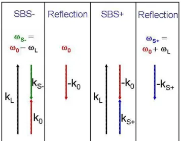
Fig. 8. Frequency and wave-number matching for generation of backscatter sidebands by stimulated Brillouin scattering (SBS). The direction of pump and upward scattered electromagnetic waves are reversed by ionospheric reflection for reception on the ground.
parameters in dispersion Eqs. (6) and (13), the signs are cho-sen to be opposite fork0 andkS to yield a low frequency
wave numberkL that has a magnitude equal to|k0−kS| in
agreement with Eq. (3).
Strictly speaking, stimulated Brillouin Scatter (SBS) is only the decay of electromagnetic waves into ion-acoustic waves and scattered electromagnetic waves. Classic treat-ments of SBS have only considered unmagnetized plasmas (Kruer, 1988). As mentioned in reference to Eq. (6), in the ionosphere when a magnetic field is imposed on the plasma the electrostatic ion cyclotron wave may also be excited by the SBS-like process. For the following discussions about Fig. 8, a generalized SBS is discussed in relation to excita-tion of the ion-acoustic wave found below the ion-cyclotron frequency and the electron ion cyclotron waves just above the ion-cyclotron frequency as shown in Fig. 6. Consequently, kLandωLare used to represent the wave number and
fre-quency of all low-frefre-quency decay products.
The wave number diagrams in Fig. 8 illustrate the SBS matching conditions. The pump frequency decay in Eq. (3) indicates a loss of EM energy from the pump to generate a low frequency ion acoustic wave. The low frequencyωL
is greater than zero and the downward scattered electro-magnetic waveωS−=ω0−ωLis downshifted from the pump
wave. The downshifted SBS- line is called the Stokes line that has a lower energy than the pump line. The resultant scattered electromagnetic wave vector is negative (or down-ward) with a value given bykS−=k0–kLsince bothk0 and
kLare upward vectors and|k0|<|kL|as shown in Fig. 8.
Af-ter reflection, downward pump wave (ω0,−k0)can split into
a down going ion acoustic away and an upward propagating scattered EM wave. After reflection, the upward EM wave is
transformed into a downshifted, down-going EM wave that adds to the scattered wave amplitude. Consequently, the wave vectors in the first panel of Fig. 8 could be reversed to represent the generation of SBS- by the reflected pump wave.
Next, the upshifted SBS+ emission is explained. The up-ward pump will reflect in the ionosphere near where refrac-tive index goes to zero yielding a downward pump wave with wave vector −k0. This reflected wave will scatter
from the ion-acoustic waves to yield an upward scattered electromagnetic wave with wave vectorkS+=k0+kL at
fre-quencyωS+=ω0+ωL. The scattered upshifted
electromag-netic wave will propagate upward until it reflects in the iono-sphere above the generation region. This wave with wave number−kS+ will propagate downward to be received on the ground as an upshifted anti-Stokes sideband of the pump wave. The SBS generation of both the Stokes and anti-Stokes lines is illustrated in Fig. 8. The anti-anti-Stokes line will have contributions from both the upgoing and downgoing, reflected pump wave.
Using Fig. 8, the Doppler shift of the anti-Stokes line (Fig. 3b) can be explained as a wave reflected by a moving reflector. For non-relativistic motion, the amount of Doppler shift (1f) for scatter from a body moving with velocity (v) is given by1f=f v?(ks
0–ki0)/cwheref is the incident
fre-quency,ks0, andki0are unit vectors in the direction of the scat-tered and incident waves, respectively (Ruck et al., 1970). As illustrated in Fig. 8, the pump wave generates the down-shifted SBS emissions without reflection and, consequently, any motion of the reflection altitude does not show up in the Stokes line. This constancy of the downshifted frequency is exactly what is shown by the blue line in Fig. 3b.
From Fig. 8, it is shown that the upshifted line is driven by the reflected pump wave. If the medium is moving downward with velocityV, the frequency of the Doppler-shifted reflected wave isω0+2V ω0/c. After scattering with
the ion acoustic waves at frequency ωIA, the
electromag-netic wave propagates upward and is reflected by the iono-sphere. The resulting upshifted wave has a frequency of ω0+ωIA+4V ω0/c. Note that the Doppler shift of the
re-flected pump wave is one-half that of the upshifted SBS line. The initially measured 5 Hz frequency offset corresponds to a Doppler motion of about 80 m/s in the HF reflection alti-tude. When the pump wave is first turned on, electron heat-ing seems to yield a lowerheat-ing in the HF reflection altitude. The positive Doppler shift from this reduction in the altitude of reflection is consistent with an initial enhancement in the plasma density near the reflection altitude. As the plasma ap-proaches thermal equilibrium, this Doppler shift in the SBS+ line is reduced to nearly zero.
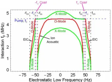
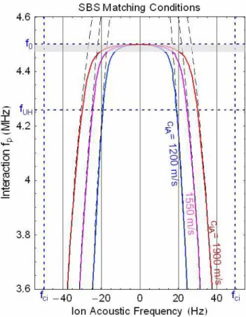
Fig. 9. Generalized SBS matching conditions for O-Mode and X-Mode electromagnetic waves at 4.5 MHz for an ionosphere with an ion sound speed of 1600 m/s and an ion gyro frequencyfci=49.6 Hz
propagating at an angle of 14.5◦with respect to magnetic field di-rection.
so kL∼=2k0. This is substituted into Eq. (6) and solved to
yield either an equation for the ion sound frequency ω2L=1
2(4c
2
IAk02+2i±
q
16c4IAk04+4i−8c2IAk022iCos2θ )(16) where the + sign represents the EIC wave and the −sign denotes the IA wave. In either case the ion sound speed is cIA2 =ω
2
L
4k02
2i−ωL2
2iCos2θ−ω2L (17) wherek02 is given by Eq. (13). With prescribed values of wave frequency, propagation angle, plasma frequency, elec-tron and ion cycloelec-tron frequencies in the interaction region, Eqs. (13) and (16) provides an accurate description of the re-lation between the ion sound speed and two possible values of low frequency waves excited by generalized SBS process. The limits to the ion sound speeds are found by substituting the free space valueω0/cfork0in Eq. (16). Those
frequen-cies are ω2M±=1
2( 4c2IAω20
c2 + 2
i
± s
16c4IAω04 c4 +
4
i−
8c2IAω022iCos2θ
c2 ) . (18)
An analytic solution to the matching equations is derived to yield insight into the SBS interactions in magnetized plasmas. The quasi-longitudinal (QL) approximations to the electromagnetic wave dispersion equations are given by Eq. (14). This is combined with Eqs. (16) and (3) to give the plasma frequency at the SBS interaction altitude
ω2p=ω0(ω0±eCosθSign[ω02−ω2p])
1− c
2ω2 IA
4c2IAω20
(2i−ω20) 2iCos2θ−ω20
!
(19)
remembering that this equation is only valid if the QL condi-tions (Eq. 15) are satisfied.
The matching conditions depend on the wave frequency, the plasma frequency and the ion-sound speed at the interac-tion region. In the ionosphere, the generalized SBS can occur at a range of electron densities corresponding to the match-ing condition plasma frequency. The ion-sound speed will be determined by the electron and ion temperatures that are elevated above ambient conditions by the electromagnetic pump wave. For electron temperatures in the range of 1000 to 4000 K and ion temperatures between 600 and 1000 K the ion-sound speedcIAtakes values from 1200 to 1900 m/s. For fixed ion-sound speeds, Eqs. (12) and (16) are used to nu-merically compute the matching plasma frequencyfpe as a
function of the matching electrostatic low frequencyfL. For
the same parameters, if the QL approximation is satisfied, Eq. (19) will provide an analytic expression of the plasma frequency corresponding to the local plasma density in the interaction region.
The computed matching conditions for the HAARP exper-imental parameters are graphed in Fig. 9 based on numerical computations with Eqs. (13) and (16). Electrostatic ion cy-clotron solutions are found for frequencies just above the ion cyclotron frequencyfci. The ion acoustic wave solution is
limited to frequencies less than the longitudinal component (fciCosθ )of the ion cyclotron frequency. The plasma
fre-quency of the SBS interaction is determined by the electron density profile. Figure 9 illustrates that both O-mode and X-mode pump waves can excite the SBS instability. For each ion sound speed there are three values of plasma frequency that provide matching, one below the pump frequency for O-mode, one below the pump frequency for X-Mode, and one above the pump frequency for X-mode. The QL approxima-tion expression (18) does not include this effect but passes through thef0=fp boundary as the sign is changed from +
for O-Mode to−for X-mode. This paper only presents data for O-Mode excitation but future experiments at HAARP will attempt to excite SBS by X-Mode waves.
To generate Fig. 9, the vertical pump wave at 4.5 MHz is assumed to propagate with an angle of 14.46 degrees with the background magnetic field. The electron and ion gyro frequencies are given by the IGRF magnetic field for the Oc-tober 2008 time period. The values representative of the con-ditions over HAARP at 178 km altitude arefce=1.457 MHz
andfci=49.6 Hz, respectively. The SBS matching conditions
are computed for a warm ionosphere with an ion sound speed of 1600 m/s. The QL-approximation to the matching condi-tions works well except where the wave frequency f0
be-comes close to the local plasma frequencyfp. The results
The low frequency solutions from O-mode interactions are restricted to the ranges 0<fIA<fM− and fci<fEIC<fM+ where fM−=45.2 Hz and fM+=60.6 Hz in this example. Only stimulated electromagnetic emissions in the ion-acoustic frequency range have been measured. With these frequency limits, the low-frequency continuum that extends out to 200 Hz in Fig. 2 cannot be produced by SBS. The next step in the theory is to determine the plasma frequencies of the regions where the electromagnetic pump interacts with the plasma.
5 The electromagnetic pump wave in the ionosphere
The HAARP HF transmissions are generated with a ground based phased array which employ 360×10 kW transmitters operating continuously. The pump signal at 4.5 MHz had an effective radiated power ofPEff=1 GW. The electric fields in the ionosphere are a standing wave composed of the up-ward wave from the transmitter and the reflected down-going wave. The electric field of the upward wave is related to the time averaged Poynting vector as
PEff
4π z2= |E|2n
η0
(20) wherezis the altitude in meters, n is the refractive index, and η0=377 ˙Ohms is the impedance of free space.
The structure of the standing wave in the ionosphere is de-termined by the background electron density profile. From the profiles in Fig. 5 for the electron densities for 19:58 UT on 24 October 2008, it was determined that the 4.5 MHz pump wave reflected in the ionosphere at the critical density of 2.51×105cm−3at an altitude (z
0)of 177.74 km.
The amplitudes of the high power electric fields are com-puted using the wave equations for vertical propagation in a horizontally-stratified, fluid plasma with a steady mag-netic field. These equations were first derived by F¨orsterling (1942) and described in great detail by Budden (1969, 1985), Yeh and Liu (1972), and Lundborg and Thid´e (1985, 1986). The second order differential equation for O-mode propaga-tion is given as
∂2F(O)(z) ∂z2 +k
(O)(z)2F(O)(z)
=0 (21)
wherek0is found from Eq. (11) including the collisional
ab-sorption terms. Coupling to a similar equation for the ex-traordinary X-mode is neglected with the smooth gradients in the F-layer profile (Yeh and Liu, 1972; Lundborg and Thid´e, 1985, 1986). The electron density profile is used to compute ak02with transition from positive to negative val-ues across the resonance altitudez0. Below this altitude, the
pump wave propagates upward and then reflects atz0to
pro-duce the down-going wave. Above the plasma resonance al-titude, the O-mode wave becomes evanescent and quickly decays. Both numerical solutions (e.g., Budden, 1969) and
approximate analytical solutions (see Lundborg and Thid´e, 1985, 1986) have been used to compute solutions to Eq. (21). In this paper, the finite difference approximations to the sec-ond derivative in Eq. (21) provide the basis for the numerical solutions.
The boundary conditions above and below the resonance altitude are specified by WKB solutions of the form
FWKB(O) (z)=F(O)(z1) s
k(O)(z
1) k(O)(z) exp
−i
z
Z
z1
k(O)(z′)dz′
(22)
wherez1is a reference altitude where the electric field
ampli-tude is specified (Yeh and Liu, 1972). The three electric field components of the wave are related to the functionF(O)(z) by the equations
{Ex(z),Ey(z),Ez(z)}
= {1,R(O)(z)−1,RL(O)} F
(O)(z)
p
R(O)(z)−2−1 (23)
where the subscripts x, y and zdenote the magnetic east, north and up directions,R(O)(z)is the O-mode polarization in Eq. (12) andPL(O)(z)is the O-mode longitudinal polariza-tion given by Eq. (4.14.22) of Yeh and Liu (1972) as RL(O)(z)= iYSinθ
(U−X)[1−n
(O)(z)2
] (24)
The transverse polarization (R(X,O)) is the ratio Ex/Ey of
the transverse electric fields. The longitudinal polarization RL(O)(z) is the ratio Ez/Ex of the longitudinal to
north-ward fields. The O-Mode and X-Mode polarizations range from circular (R(X,O)=±i) near the reflection point to linear (R(X,O)=∞or 0) near the reflection point. The longitudi-nal polarization is only large near the reflection point. The electric field component along the direction of the magnetic field is give by E||(z)=Ez(z)Cosθ−Ey(z)Sinθ whereθ is
again the complement of the magnetic dip angle. Excellent descriptions of these features are provided by Budden (1966, 1985), Yeh and Liu (1972), and Lundborg and Thid´e (1985, 1986).
The numerical solution to Eq. (21) starts at altitude z1=0.97z0=172.4 km with an upward propagating wave with a transverse electric field of 1.29 V/m corresponding to 1 GW ERP at 4.5 MHz in the ionosphere neglecting any D-region absorption. The computation is terminated at the altitude z2=1.01z0=179.5 km where the wave is strongly damped in
the overdense plasma layer. Pump wave reduction by mode conversion on field aligned irregularities at the UH resonance altitude is not included in the computation. The plasma fre-quency profile and the computed horizontal/transverse (Ex,
Ey)and vertical/logitudinal (Ez)electric fields are illustrated
in Fig. 10.
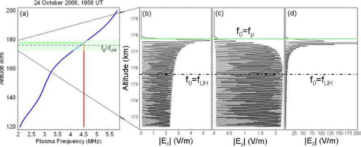
Fig. 10. Plasma frequency profile(a)and computed transverse (b, c) and longitudinal(d)electric fields produced by the 4.5 MHz HAARP transmitter. The maximum electric field is found in the longitudinal componentEz=671 V/m just below the plasma resonance at 177.74 km
altitude where the local plasma frequency is 4.48 MHz. For reference, the altitude where the wave frequency matches the upper hybrid frequency is shown with the horizontal dot-dashed line.
Similar effects have been computed by Lundborg and Thid´e (1985, 1986) using the uniform approximation technique. The peak transverse field is 5.5 V/m at 177.7 km altitude, 0.04 km below the plasma resonance altitude. The peak vertical/longitudinal electric field is 671 V/m at 177.55 km, 0.19 km below the plasma resonance altitude. For such large field strengths, the plasma will be strongly modified and the linear dispersion equations used to describe the matching conditions will no longer be valid. Outside this narrow re-gion, the electric fields are on the order of a few V/m and the matching equations remain valid. The computation used 10 000 points along the vertical axis and the simulation code was checked using know analytic Airy function solutions to linear variations ink02.
The details of the three electric field components near the reflection altitude are given in Fig. 10b, c, and d. The mag-netic east componentExand the magnetic north component
Ey are transverse to the direction of propagation. Their
am-plitudes increase as the reflection altitude is approached but the upward longitudinal component along the direction of propagation has the largest electric field (Fig. 10d). This extremely large longitudinal field could easily couple into longitudinal ion sound waves and a down-going longitudinal component of an O-Mode electromagnetic wave.
The wave matching conditions used in the previous section use both frequency and wave number matching. The stand-ing wave ripples illustrated by Fig. 10 shows that at the upper hybrid resonance level the wave number (or inverse wave-length) is well defined with upgoing and downgoing waves producing electric field pattern. Near the reflection height were the pump wave grows to over 670 V/m, the single peak is not well represented by a wave number. In this region, a full nonlocal treatment is needed to determine the coupling between high frequency EM waves and the low frequency
electrostatic wave. A full wave treatment of this process will be explored in a future paper.
Soon after the pump wave is turned on, field aligned regularities form in the F-layer and interactions at these ir-regularities absorb the wave energy to prevent pump EM wave from reaching the reflection altitude. Many of the SEE observations have led to the interpretation that much of the EM pump wave energy is deposited near the upper hybrid level where the wave frequency is equal to the up-per hybrid frequency (Leyser, 2001). The horizontal dashed line in Fig. 10 provides the location of the upper hybrid altitude (zUH=174.6 km) where ω20=ωUH2 =ω2p+2 using a
pump frequency of 4.5 MHz and an electron gyro frequency of 1.457 MHz. This value offce was based on the magnetic
field from the IGRF model. At the upper hybrid altitude, the pump wave has both transverse and longitudinal components of comparable amplitudes. For the simulation illustrated in Fig. 10, the peak electric fields near the UH resonance al-titude are (Ex, Ey, Ez)=(2.22, 2.49, 2.33) V/m. The next
section examines whether interactions near the plasma wave reflection altitude or near the upper hybrid resonance altitude produce the SBS emission lines.
6 Altitude profiles of the scattered electromagnetic waves for vertical beams
In this section, the ion-acoustic SBS matching conditions will be used to determine the altitude of the observed scat-tered EM waves for vertical propagation in a horizontally stratified ionosphere. It will be shown that the fields driving the instability can be the large longitudinal electric fields near the plasma frequency resonance altitude or the transverse and longitudinal electric field components near the upper hybrid resonance altitude. Since all the observed frequency offsets of the scatter electromagnetic waves are less than the ion cy-clotron frequency, the possible presence of electrostatic ion cyclotron waves will not be considered in this section. Con-sequently, the subscript IA will be used in place of the sub-scriptLto designate ion acoustic frequencies and wave num-bers.
The scattered EM wave is offset by the pump wave by the ion acoustic frequency according to Eq. (3). All of the ion-acoustic offsets for the scattered EM wave illustrated in Figs. 2 and 4 are less than the ion cyclotron frequency of 49.6 Hz at the reflection altitude. To map the ion acoustic frequencies determined by subtracting the pump frequency from the scattered frequency, then Eq. (17) is rearranged to give the electromagnetic wave number
k20= ω 2 IA
4cIA2
2i−ωIA2 2iCos2θ−ω2
IA
(25)
and that wave number is used in Eq. (13) to give the plasma frequency at the SBS interaction region. The map-ping curves between the ion acoustic frequencies and the ionospheric plasma frequency are given in Fig. 11 for the HAARP experiment parameters using a range of ion-sound speeds. Since the ion acoustic frequencies for interactions at the UH levels from the HAARP SEE data are between 27 and 32 Hz, the solutions with temperatures correspond-ing to an ion sound speed less than 1500 m/s are ruled out. The two interaction levels where (1) the wave frequency is slightly less than the local plasma frequency orω0=ωp and
(2) the wave frequency equals the local upper hybrid fre-quency areω20=ω2UH=ω2p+2 are indicated on Fig. 11 by horizontal dashed lines. The upper hybrid level is given by ωp=(ω20−2)1/2=26.75×106rad/s or 4.26 MHz. The upper hybrid matching level is important because the pump wave strongly interacts with the plasma at this level in conjunction with field aligned irregularities produced by the HF beam (Leyser, 2001).
The black dashed curves in Fig. 11 show the QL solu-tion (19) for the same condisolu-tions. The QL approximasolu-tion to the O-mode matching conditions for SBS is usable near the point (fUH)where the wave frequency is equal to the
lo-cal value of the upper hybrid frequency. The QL curves are asymptotic to the full solution for each ion-acoustic speed in regions below the reflection height wheref0=fp.
Fig. 11. SBS matching conditions for the O-mode pump at 4.5 MHz. The measured SBS lines with 29 Hz ion-acoustic offsets (Fig. 2) are consistent with an ion acoustic speed of 1900 m/s. The black dashed lines are the QL solution for the matching conditions for both O-mode and X-mode. The shaded portion of the figure shows where the strongest longitudinal wave can excite ion acous-tic waves by SBS. The frequencyfUH denotes plasma frequency were the wave frequency is equal to the upper hybrid frequency.
Figure 11 shows that if the SBS excitation of the scat-tered EM waves occurs close to but just below the plasma frequency resonance atf0, the ion acoustic frequency will be
Fig. 12. Reconstructed profiles of scattered O-mode waves in the ionosphere. The upshifted and downshifted SBS ion-acoustic lines from Fig. 2c are first mapped to(a)the plasma frequency using the matching conditions for SBS with the assumption of a 1900 m/s ion sound speed. The measured electron density profiles in Fig. 5 relate the local plasma frequency to the altitude yielding(b)the altitude profile of scattered EM wave power. The maximum scattered wave coincides with the location of the upper hybrid resonance.
temperature of 11 500 K. Any changes in the ion-acoustic speed at the UH level become manifested as changes in the ion-acoustic frequency offset of the SBS EM wave.
The next step is to use the map between ion acoustic fre-quency and interaction plasma frefre-quency to produce a pro-file of the scattered wave power in the ionosphere. For downshifted and upshifted SBS lines shown in Fig. 2a, the matching conditions yield the scattered wave power profiles shown in Fig. 12. The plasma frequency profile is determined using the mapping function withcIA=1900 m/s. This
ion-acoustic speed provides a good match between the measured ion-acoustic peak frequency and the SBS matching condition curve. The altitude profile is obtained with electron density profile at 19:48 UT from Fig. 5 where the electron density is converted to plasma frequency. This plasma-frequency pro-file determination depends on the assumptions that (a) the heated electron and ion temperatures give an ion sound speed of 1900 m/s and (b) that the electron density profile has not been modified by the HF facility to significantly distort the values given in Fig. 5.
The top of Fig. 12 is just below the reflection altitude where the pump wave fields shown in Fig. 10 reach their maximum. With the assumed 1900 m/s ion-sound speed, the peak scattered fields are very close to the altitude of the upper hybrid wave resonance with the pump wave. This mapping shows a broad region around the UH altitude for scattering of the EM pump wave by SBS. The concept is that the EM pump amplitude is depleted over the large a 6-km region near the UH resonance altitude before approaching the reflection altitude. The ion acoustic speed parameter,cIA, can be
ad-justed to place the scattered wave peak at the UH altitude. Similarly, lowering the sound speed to 1887 m/s brings the peak of the downshifted SBS profile to the UH level. Near the UH level, the matching curves in Fig. 11 are more vertical than near the reflection altitude. The estimated value for ion-sound speed is insensitive to variation in altitude around the UH level. The SBS instability seems to be occurring near the UH altitude (zUH)were the wave frequency is equal to the lo-cal upper hybrid frequency. At this altitude, it has been pos-tulated that the electromagnetic pump wave decays into up-per hybrid and lower hybrid waves and that the upup-per hybrid waves mode converts to an electromagnetic wave to be re-ceived on the ground as the downshifted maximum (DM) in the spectrum of stimulated electromagnetic emissions (SEE) (e.g. Leyser, 2001). The results of Fig. 12 suggest that, for high enough power pump wave, the SBS instability is also excited around the UH level to produce the observed SBS spectral lines in the SEE.
If the SBS emissions come from the UH level, a simple ex-pression for the ion sound speed can be derived. The QL ap-proximation given by Eq. (19) is valid at the UH matching al-titude. The UH level is defined by the conditionω20−2e=ω2p. Substituting this into Eq. (19) for the O-mode and solving for cIAyields.
cIA= cωIA 2√eω0
v u u t
2i−ω20 2iCos2θ−ω20
s
ω0+eCosθ
ω0Cosθ+e
(26)
At 19:56 UT, the measured upshifted ion acoustic frequency is fIA=29.2 Hz or ωIA=183.5 rad/s. (Note: Frequency in Hz is only used for comparison to the measured frequency offsets in the scattered SBS lines). The computed elec-tron and ion cycloelec-tron frequencies are e=9.16×10⁶rad/s,
i=312 rad/s and magnetic field angle from verticalθ=14.5◦
based on the magnetic field components from the IGRF model at 175 km altitude. With these parameters and us-ing the pump frequencyf0=4.5 MHz orω0=28.3×10⁶rad/s,
Eq. (26) gives an ion sound speed ofcIA=1812 m/s. Similarly
the downshifted ion acoustic frequency of−30 Hz yields an ion sound speed of 1865 m/s. These values are both about 2.5% lower than those using the more accurate formulas (13) and (16).
Table 2. Electron temperatures determined from Stimulated Bril-louin Scattering for vertical heating of the ionosphere at 4.5 MHz.
Time (UT) 19:48 19:58 Line SBS− SBS+ SBS− SBS+ fIA(Hz) −30.6 30.6 −29.2 27.8 CIA(m/s) 1780 1780 1690 1580 Te(K) 3500 3500 3180 2870
Te=3Ti which is a sufficient condition for prevention of
Lan-dau damping of ion acoustic waves. Te=
mic2ω2IA
(γe+γi/3)4eω0
2i−ω02 2iCos2θ−ω02
ω0+eCosθ
ω0Cosθ+e
(27) Table 2 gives the values for ion-acoustic speed and elec-tron temperature obtained from Eqs. (26) and (27), respec-tively, using the ion acoustic frequency data of Table 1 and the other parameters previously given for the HAARP ex-periment. Only the vertical beam observations are used be-cause theory was developed for vertical incidence on a hor-izontally stratified layer. The changes in the electron tem-peratures show a drop of about 500 K for the 10 min interval between the two HF experiments. With an estimated accu-racy of 0.7 Hz for the SBS frequencies, the uncertainty for the recovered ion sound speed is1cIA=50 m/s and for
elec-tron temperature is1Te=200 K. The assumption ofTe=3Ti
makes the ions sound speed determination more reliable than the electron temperature measurements. ThisTe
determina-tion can be improved by considering the thermal coupling between the electrons and ions. The factors that cause the ap-parent electron temperature to drop over a period of 10 min are (1) change the coupling to the plasma by variations in the altitude profile of the F-layer or (2) change in the effective heating by increased D-region absorption. These processes that affectTe should be studied in the future with physics
based models.
The measurement technique embodied in Eqs. (26) and (27) should be robust against variations in the actual SBS production efficiency. Even if the ion-acoustic waves are heavily Landau damped (whenTe∼Ti)or damped by
ion-neutral collisions, the SBS instability can proceed if the scattered pump wave is not strongly damped (Kruer, 1988; Eliezer, 2002). With damped ion-acoustic waves, the SBS is local but growing. The threshold conditions for the SBS instability in a magnetized plasma needs to be developed to fully understand the pump wave fields needed to produce the low-frequency SEE observations.
7 SBS matching at the magnetic zenith
The examples considered thus far for SBS measurements were made with a vertical beam in a horizontally stratified
Fig. 13. Ion acoustic (IA) and Electrostatic Ion Cyclotron (EIC) wave matching frequencies(a)and ray paths(b)for the 5.6 MHz wave propagating to the vertical (red) and to the magnetic zenith. When the paths of either ray cross the upper hybrid resonance re-gion, nearly the same ion-acoustic frequency can be excited.
ionosphere. If the HF beam is tilted off vertical, the wave normal angle relative to the magnetic field direction will vary with altitude. Raytracing in the anisotropic plasma can pro-vide both the wave number magnitudek0and the wave
nor-mal angleθ. These quantities can be substituted in Eq. (17) to give the relationship between the ion sound speed and the ion acoustic frequency along the ray propagation path.
The Hamilton’s equations for ray paths using the refractive index in a magnetized plasma (Eq. 13) are given by Hazel-grove (1955), Yeh and Liu (1972) and Budden (1985). These equations were solved numerically for propagation in the measured ionosphere over the HAARP transmitter. The O-Mode raytrace results for 5.6 MHz are illustrated in Fig. 13. The electron density is given by the purple shading on the right. The vertical ray shown in red keeps the same wave normal angleθthroughout the propagation because the mag-netic field direction is nearly constant with altitude relative to the vertical wave-propagation direction. The physical path bends slightly to the north near the reflection altitude.
The finite width of the beam may allow scattering of dis-placed downward EM waves from the center by ion-acoustic waves excited by high power EM waves at the edge.
Two sets of matching conditions are illustrated in the left panel of Fig. 13. The electron ion cyclotron (EIC) wave can yield waves in the 50 to 70 Hz range. These waves have not been detected in the observations. The set of matching con-ditions for frequency offsets of 50 Hz or less come from the ion acoustic waves. These are the waves recorded by ground SEE measurements. At the upper hybrid altitude the SBS matching conditions (Eq. 17) are nearly identical for both the vertical and MZ ray paths along the upward trajectories (Fig. 13 left). For those rays and the same electron temper-atures or ion sound speeds, the ion acoustic frequencies for the SBS-2 lines should be nearly identical. This may account for the consistency in the downshifted SBS peak frequencies given by Table 1.
The upshifted SBS line for vertical pump waves shows ev-idence of Doppler motion of the ionospheric reflection sur-face. As illustrated by the temporal variations in Fig. 3 and discussed in Sect. 4, the reflected pump and scattered EM waves combine to produce upshifted SBS lines with slightly higher than the offsets of the downshifted SBS lines. A slight reduction of the ionosphere reflection level may occur just after the high power HF by a localized region of enhanced ionization. The reflected EM waves are then Doppler shifted by this lowering in the reflection altitude. Future experiments should investigate the initial shifts in the SBS lines to confirm this observation.
With the wave number and propagation angle provided by raytracing, the electron temperature measurement technique can be extended for use at regions where the SBS is excited just below the pump reflection altitude at the magnetic zenith. During the time period around 19:30 UT on 24 October 2008, the HAARP transmitter was operated at full power to provide 1.66 GW at 5.6 MHz. The measured SEE spectra during that time showed strong SBS-1 lines with an downshifted peak at−14.5 Hz and two upshifted SBS lines SBS+1 at 17.5 Hz and SBS+2 at 36.0 Hz as previously shown by Fig. 4. The downshifted SBS line from the UH altitude region is proba-bly masked by the strong downshifted SBS-1 emission.
To support the 5.6 MHz observations, rays were propa-gated with the measured electron density profile given in Fig. 5. With the raytracing solution, the values of O-Mode wave numberk0and the propagation angleθare used with
Eq. (16) to compute the ion acoustic frequency that satisfies the SBS matching conditions. As with 4.5 MHz, the 5.6 MHz pump wave provides nearly identical ion acoustic wave fre-quencies at the upper hybrid resonance altitude. Compared to the 4.5 MHz results, there is a larger band of ion-acoustic waves that satisfy the SBS matching conditions in a band be-tween−10 to−20 Hz. This may account for the large spread in the downshifted SBS line as illustrated in Fig. 4.
The wave-matching conditions for the 5.6 MHz pump were computed using the theory of the Sect. 3 neglecting the
Fig. 14.Transfer of the low-frequency emission peaks from stimu-lated Brillouin scatter to the plasma frequencies in the ionospheric interaction regions. The top matching curve is computed assuming the ion-sound speed has a constant value of 2050 m/s throughout the interaction region in the plasma.
tilt of the ray path. The results of this computation were com-pared to the measured SBS spectrum yielding an estimate of the plasma frequency at the interaction regions. The mapping between the ion-acoustic frequency offsets of the observed SBS spectra and the plasma frequency required for match-ing is illustrated in Fig. 14. The ion-sound speed (2050 m/s) was adjusted to match the measurements for the SBS+2 peak with the theoretical transfer-function at the upper-hybrid al-titude. The inflection in the downshifted side of the spectra near−30 Hz maps an SBS-2 region that is masked by the strong SBS-1 emission.
Fig. 15. Electromagnetic emission lines from the SBS spectrum mapped to the source altitudes for a magnetic zenith pump wave at 5.6 MHz. The two separate lines come from two distinct altitude regions. The peak strength is just below the reflection level and the dot-dash line is at the upper hybrid resonance altitude. The altitude determination is obtained from an assumed electron density profile.
are observed, the EIC portion of the matching curve is not shown. The SBS-1 and SBS+1 lines are much stronger than the corresponding lines (SBS-2 and SBS+2) from the UH level because the pump amplitude is much weaker at the UH level than near the reflection level where the plasma fre-quency is nearly equal to the 5.6 MHz pump frefre-quency.
Each feature of the SBS frequencies is transferred to the profile of the backscattered EM emission source region (Fig. 15). The maximum intensity of the SBS lines maps well to the altitude profiles of Sect. 5 where the strong max-imum EM wave is expected just below the reflection level. The much weaker scatter EM wave is expected at the UH level where the pump is much weaker. The UH resonance in-teractions occur when the ion sound speed is set to 2050 m/s. This corresponds to an electron temperature of 4000 K us-ing the assumptions for Eq. (27) along with the assump-tion that the elevated electron temperature is constant along a magnetic field line. With these measurements, it seems that the electron temperature at 19:38 using 5.6 MHz with 1.66 GW ERP produced a substantially larger electron tem-perature (∼4000 K) than was observed 10 and 20 min later with 4.5 MHz at 1.0 GW ERP (∼3000 to 3500 K).
8 Summary and conclusions
This paper has provided experimental measurements of stim-ulated Brillouin scatter supported by wave matching the-ory and ray tracing. The measurements of stimulated Bril-louin scattering have been made using a digital sampling
re-ceiver located near the HAARP high power HF transmitter in Alaska. The emissions seem to originate either from the upper hybrid level or from the pump-maximum altitude just below the O-mode reflection or plasma-resonance level. The SBS data taken over a 20 min period from 19:40 to 20:00 UT (11:20 to 12:00 Local Time in Alaska) only show both down-shifted (SBS-) and updown-shifted (SBS+) lines from near UH res-onance region with 30 Hz offsets from the pump wave. In all cases with a 4.5 MHz pump, the upshifted, anti-Stokes line is between 4 and 8 dB weaker than the downshifted, Stokes line. The positions of the lines do not show signifi-cant change either when the power of the pump is dropped for the vertical beam or when the full power pump is tilted toward the magnetic zenith.
The SBS data at 5.6 MHz show strong interactions near the reflection level for magnetic zenith heating. This effect lasted for 20 min between 19:20 and 19:40 UT. The Stokes line was 37 dB larger than the anti-Stokes emission. A weak upshifted SBS+2 line in the spectra is located at an ion-acoustic fre-quency that is consistent with SBS matching conditions at the UH resonance altitude.
All the spectra also show a low frequency continuum extending ±200 Hz from the pump frequency. The inten-sity of this low-frequency continuum is also larger on the downshifted side than the upshifted side of the pump wave. The low-frequency continuum cannot be produced by the SBS generation of either ion acoustic or electrostatic-ion cy-clotron waves because the matching conditions do not per-mit frequencies abovefM+=61 Hz. The source of this con-tinuum could be low-level spurious noise from the HAARP transmitter.
The theory for stimulated Brillouin scattering has been ap-plied to regions of the ionosphere where the electromagnetic pump frequency exceeds the local value of plasma frequency. During SBS, the pump wave decays into a backscattered EM photon and a low-frequency phonon. Energy and momentum conservation as represented by the wave-wave interactions define the properties of the scattered electromagnetic wave. The conservation laws (Eq. 3) and dispersion equations for the low-frequency electrostatic wave (Eq. 6) and the scat-tered electromagnetic wave (Eq. 13) are solved to give the relationship between the plasma frequency (or plasma den-sity) where the SBS interaction is occurring and the low fre-quency offset of the scatter EM wave. The matching condi-tions are dependent on (1) the ion sound speed in the plasma, (2) the electron and ion gyro frequencies, (3) the propagation angle relative to the magnetic field, and the EM pump fre-quency. For the generalized SBS in a magnetized plasma, low-frequency electrostatic wave can be either an electro-static ion cyclotron wave with a frequency just above the ion cyclotron frequency (i) or ion-acoustic wave with a
fre-quency belowi. Only SBS associated with ion acoustic