Coherent uncertainty analysis of aerosol measurements from multiple satellite sensors

(1)

www.atmos-chem-phys.net/13/6777/2013/ doi:10.5194/acp-13-6777-2013

Atmospheric

Chemistry

and Physics

Geoscientiic

Coherent uncertainty analysis of aerosol measurements from

multiple satellite sensors

M. Petrenko1,2and C. Ichoku2

1_{Earth System Science Interdisciplinary Center, University of Maryland, College Park, Maryland, USA} 2_{NASA Goddard Space Flight Center, Greenbelt, Maryland, USA}

Correspondence to:M. Petrenko (maksym.petrenko@nasa.gov)

Received: 31 January 2013 – Published in Atmos. Chem. Phys. Discuss.: 18 February 2013 Revised: 12 June 2013 – Accepted: 13 June 2013 – Published: 22 July 2013

Abstract.Aerosol retrievals from multiple spaceborne

sen-sors, including MODIS (on Terra and Aqua), MISR, OMI, POLDER, CALIOP, and SeaWiFS – altogether, a total of 11 different aerosol products – were comparatively analyzed us-ing data collocated with ground-based aerosol observations from the Aerosol Robotic Network (AERONET) stations within the Multi-sensor Aerosol Products Sampling Sys-tem (MAPSS, http://giovanni.gsfc.nasa.gov/mapss/ and http: //giovanni.gsfc.nasa.gov/aerostat/). The analysis was per-formed by comparing quality-screened satellite aerosol opti-cal depth or thickness (AOD or AOT) retrievals during 2006– 2010 to available collocated AERONET measurements glob-ally, regionglob-ally, and seasonglob-ally, and deriving a number of statistical measures of accuracy. We used a robust statisti-cal approach to detect and remove possible outliers in the collocated data that can bias the results of the analysis. Over-all, the proportion of outliers in each of the quality-screened AOD products was within 7 %. Squared correlation coeffi-cient (R2) values of the satellite AOD retrievals relative to AERONET exceeded 0.8 for many of the analyzed prod-ucts, while root mean square error (RMSE) values for most of the AOD products were within 0.15 over land and 0.07 over ocean. We have been able to generate global maps show-ing regions where the different products present advantages over the others, as well as the relative performance of each product over different land cover types. It was observed that while MODIS, MISR, and SeaWiFS provide accurate re-trievals over most of the land cover types, multi-angle capa-bilities make MISR the only sensor to retrieve reliable AOD over barren and snow/ice surfaces. Likewise, active sensing enables CALIOP to retrieve aerosol properties over bright-surface closed shrublands more accurately than the other

sensors, while POLDER, which is the only one of the sen-sors capable of measuring polarized aerosols, outperforms other sensors in certain smoke-dominated regions, including broadleaf evergreens in Brazil and South-East Asia.

1 Introduction

(2)

un-der what circumstances each of these products provides the greatest accuracy.

The unique attributes of a particular sensor may be ad-vantageous for aerosol retrievals, depending on the parame-ter(s) being retrieved, especially under favorable atmospheric conditions. However, aerosol retrieval accuracy can also be affected by numerous other factors, including the retrieval algorithm’s assumptions and parameterizations, the instru-ment characteristics (intrinsic design, calibration, and time-dependent degradation), the measurement configurations (so-lar and view geometry), the atmospheric conditions (cloudi-ness, aerosol mixing, layer height, and humidity), the sur-face background (vegetated, bare, snow-covered, inundated, or simply just dark or bright land surface or ocean), and oth-ers (Kokhanovsky et al., 2007).

Since the accuracy of aerosol retrieval from a sensor may be affected positively or negatively by these factors and con-ditions in different ways and to varying degrees, a syner-getic use of similar aerosol parameters across the sensors is non-trivial, and the data synergy research is instead focused on combining orthogonal (i.e., non-conflicting) aerosol mea-surements. For example, the aerosol layer height informa-tion from the Cloud-Aerosol Lidar with Orthogonal Polariza-tion (CALIOP) has been used to enhance aerosol retrievals from other sensors (Oo and Holz, 2011; Torres et al., 2012; Zhang et al., 2011), while the geometry information from the Advanced Along Track Scanning Radiometer (AATSR) was used to initialize the Moderate Resolution Imaging Spec-troradiometer (MODIS) bidirectional reflection distribution function (BRDF) in order to derive AATSR AOD (Guo et al., 2009).

To characterize better the differences and uncertainties that exist between the aerosol retrievals from different sensors, several studies compared a limited number of sensors. For example, AOD retrievals from MODIS were separately com-pared to retrievals from the MISR Multi-angle Imaging Spec-troradiometer (Kahn et al., 2007, 2011; Mishchenko et al., 2010; Zhang and Reid, 2010), the POLDER – POLarization and Directionality of the Earth’s Reflectances sensor (Gérard et al., 2005), and CALIOP(Kittaka et al., 2011; Redemann et al., 2012). A larger set of sensors was intercompared using a synthetic benchmark (Kokhanovsky et al., 2010), and also based on detailed analysis of data from limited geographi-cal regions (Cheng et al., 2012; Yu et al., 2012). In addi-tion, a set of 9 aerosol products was evaluated over ocean and coastal AERONET (Aerosol Robotic Network) sites dur-ing the period of 1997–2000, highlightdur-ing regions of high retrieval agreement and disagreement (Myhre et al., 2005). However, all the satellite data used in that study had already undergone post-retrieval spatiotemporal aggregation at 1×1

degree grid resolution on a monthly mean basis (so-called Level 3 products) before they were used in the comparisons. Finally, a recent study compared AERONET retrievals with a set of 5 spaceborne aerosol products archived at the ICARE Data and Services Center, including POLDER,

MODIS-Aqua (Dark Target retrievals), MERIS, SEVIRI, and CALIOP (Bréon et al., 2011). Although that study was based on a similar collocation framework as that used in the cur-rent study, our study focuses on a diffecur-rent set of sensors that provides a more extensive set of over-land spaceborne aerosol products. Furthermore, the presented study is based on the analysis of the spatiotemporally averaged and outlier-screened data, whereas that of Bréon et al. (2011) is predomi-nantly based on the analysis of individually collocated space-borne and ground-based data points that are the closest in space and time that would correspond to the central values in our collocated data subsets (we report a similar analysis in the Supplement to this paper).

In this work, 11 retrieval-scale (Level 2) aerosol products from multiple spaceborne sensors are intercompared dur-ing the recent “golden” period of 2006–2010 (see Fig. 1), when as many as seven major sensors were in operation and measuring aerosols concurrently. Specifically, we focus on aerosol products retrieved over land and ocean from MODIS on Terra and Aqua, MISR on Terra, the Ozone Monitor-ing Instrument (OMI) on Aura, POLDER on PARASOL, CALIOP on CALIPSO, and the Sea-viewing Wide Field of view Sensor (SeaWiFS) aboard the SeaStar spacecraft. At the time of this study (January 2013), all of the stud-ied sensors were still active, with the exception of SeaW-iFS, whose operation ended in December 2010. The analy-sis is based on the collocation of the satellite data products using the Multi-sensor Aerosol Products Sampling System (MAPSS) framework (Petrenko et al., 2012), which samples these satellite products relatively uniformly over the global AERosol Robotic NETwork (AERONET) of sun photome-ters and other important ground-based stations both over land and ocean.

The details of the MAPSS sampling approach are ex-plained in Sect. 2, while the relevant characteristics of the aerosol data products from the different sensors and the cor-responding data quality screening techniques are described in Sect. 3 and Sect. 4. Section 5 describes a novel statistical ap-proach for detecting and removing possible data outliers that can exist in the collocated data and, as a result, bias the sta-tistical analysis of these data. Section 6 presents the detailed analysis of the compared aerosol products, while Sect. 7 ex-amines the accuracy of these products based on land cover type. Conclusions are presented in Sect. 8.

2 Sampling method

(3)

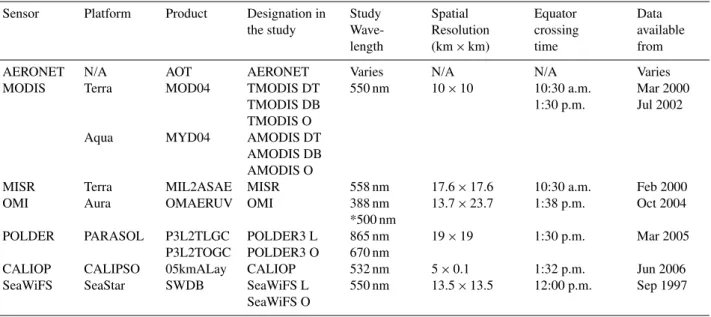
Table 1.Ground-based and spaceborne atmospheric aerosol products analyzed in the study. In the product designation titles, “O” at the end

of the title of a product signifies ocean retrievals, “L” – land retrievals, “DT” – land retrievals using the MODIS Dark Target algorithm, and “DB” – land retrievals using the MODIS Deep Blue algorithm. The AERONET AOD retrievals were interpolated to the studied wavelengths of the spaceborne sensors. The indicated local equatorial crossing times (LT) are based on the original orbital designs, and can change during the lifetimes of the satellites. SeaWiFS mission has ended in December 2010. * While 388 nm was the main observational wavelength used in the study for OMI, 500 nm was used where the collocated AERONET data were not available in the UV range.

Sensor Platform Product Designation in the study Study Wave-length Spatial Resolution (km×km)

Equator crossing time Data available from

AERONET N/A AOT AERONET Varies N/A N/A Varies

MODIS Terra MOD04 TMODIS DT 550 nm 10×10 10:30 a.m. Mar 2000

TMODIS DB 1:30 p.m. Jul 2002

TMODIS O

Aqua MYD04 AMODIS DT

AMODIS DB AMODIS O

MISR Terra MIL2ASAE MISR 558 nm 17.6×17.6 10:30 a.m. Feb 2000

OMI Aura OMAERUV OMI 388 nm

*500 nm

13.7×23.7 1:38 p.m. Oct 2004

POLDER PARASOL P3L2TLGC P3L2TOGC

POLDER3 L POLDER3 O

865 nm 670 nm

19×19 1:30 p.m. Mar 2005

CALIOP CALIPSO 05kmALay CALIOP 532 nm 5×0.1 1:32 p.m. Jun 2006

SeaWiFS SeaStar SWDB SeaWiFS L SeaWiFS O

550 nm 13.5×13.5 12:00 p.m. Sep 1997

1996 1998 2000 2002 2004 2006 2008 2010 2012 MISR MODIS Terra MODIS Aqua OMI POLDER 3 CALIOP SeaWiFS POLDER 1 POLDER 2

Fig. 1. Periods of operation of major past and current

aerosol-measuring satellite sensors. The pair of dotted vertical lines marks the “golden” period (between the start of CALIOP in July 2006 and the end of SeaWiFS in December 2010) when as many as seven of these sensors were measuring aerosols concurrently. The golden pe-riod was used as the base for the studies reported in the rest of this paper.

AERONET and for comparison with one another, we used the framework of Multi-sensor Aerosol Products Sampling System (MAPSS) that was originally developed by Ichoku et al. (2002) for validation and analysis of MODIS aerosol products (Chu et al., 2002; Ichoku et al., 2003, 2005; Levy et al., 2010; Remer, 2002) and later expanded to support aerosol products retrieved by other spaceborne sensors (Petrenko et al., 2012). MAPSS subsets the aerosol products by extracting pixels covering approximately the same area on the ground centered over AERONET sun photometer measurement sites and over certain other point locations that are not addressed in this study.

Assuming an imaginary circle of 55 km diameter whose center coincides with each AERONET station, all space-borne aerosol product pixels falling within the circle are ex-tracted. An aerosol pixel is regarded as being within the circle if the coordinates of the pixel center fall within 27.5 km from the coordinates of the circle center, where the distance be-tween the coordinates of the two points is determined using the Haversine formula (Sinnott, 1984). Based on the nomi-nal spatial resolution of the sensors in Table 1, the approxi-mate maximum number of pixels within the 55 km diameter sample space at nadir for the different sensors is as follows: MODIS – 25, MISR – 9, OMI – 8, POLDER – 9, CALIOP – 11, and SeaWiFS – 16. The actual number of pixels within the sampling circle decreases for the aerosol retrievals away from the nadir of the satellite scene, and can be further duced in the presence of clouds or other factors preventing re-trieval of aerosol parameters. Based on the extracted sample, statistics of each aerosol parameter retrieved within the sam-pling areas are calculated and include mean, median, stan-dard deviation, as well as the value of the central point in the sample, i.e., the pixel in the spaceborne subset that is the clos-est (i.e., whose center has the smallclos-est distance) to the ground station, or the individual data point in the ground-based sub-set that is measured the closest in time to the overpass of the satellite.

(4)

Supplement to this paper. It is appropriate to use the mean values in this paper, so as to maintain the uniform sampling criterion across the different sensors and their respective re-trieval pixel sizes to facilitate a fair intercomparison. On the other hand, an analysis based on the central pixel values such as that reported in the Supplement can provide further details on the effect of difference in sampling aerosol products from individual sensors, as well as more accurately characterize the performance of the sensors in the presence of a strong point source of pollutant particles. Additionally, it should be noted that since the mean value of a sample can be computed even if its central value is missing, the reported analysis of the central values is based on a somewhat reduced volume of the collocated data points when compared to the reported analysis based on the mean values.

To collocate AERONET data in time and space with the satellite data, AERONET measurements acquired within

±30 min of each satellite sensor overpass are also extracted

and the corresponding statistics are derived. Additionally, for the convenience of aerosol data intercomparison and valida-tion, AERONET AODs are interpolated to the wavelengths of spaceborne sensors in Table 1 based on the established wavelength dependence of AOD (Eck et al., 1999). It is per-tinent to note that this interpolation process might introduce an additional source of uncertainty when intercomparing the aerosol products. Also, because of the wavelength depen-dence of AOD, the difference in the compared wavelengths of the spaceborne products should be considered when in-tercomparing the relative performance of the products. Fur-thermore, although many AERONET stations provide obser-vations in the range of 340–1020 nm, certain stations report AOD in the range of 440–1200 nm. For such stations that have no measurements in the UV region, we have evaluated OMI AOD at 500 nm instead of AOD at 388 nm, in order to avoid additional extrapolation biases.

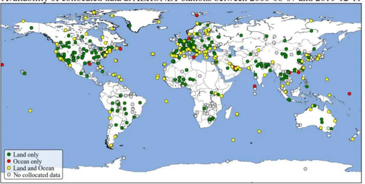
Each AERONET station has a different period of opera-tion, and the quantity of available AOD data points is not uniform across all stations; while many stations are still ac-tive, certain stations were active in the past and only for a short period of time. The overall availability of the col-located data during the analysis period of 2006-06-07 to 2010-12-11 is shown in Fig. 2, where for the purposes of this study the stations are classified as land-only, oceonly, or land-and-ocean. This classification is based on an-alyzing collocated data of separate aerosol retrievals over land and ocean from the MODIS, SeaWiFS, and POLDER sensors and identifying stations that have AOD data points from the land datasets, ocean datasets, or both; note that the MISR, OMI, and CALIOP sensors provide only joint land-and-ocean datasets.

3 Aerosol products

The key properties of the 11 analyzed aerosol products are summarized in Table 1, while the original science dataset (SDS) names of the spaceborne aerosol products are out-lined in the first column of Table 2, except for the POLDER products that do not have an established SDS product nam-ing convention. The sampled satellite data products are de-rived directly from the retrieval level aerosol products (Level 2) that represent the highest available spatial resolution for each product/sensor combination and are free of aggregation artifacts that can be present in data at Level 3 (Hyer et al., 2011; Levy et al., 2009; Zhang and Reid, 2010).

Of the 11 sampled products, 3 are combined land-and-ocean products, 6 land-only products, and 4 land-and-ocean-only prod-ucts. Furthermore, 6 aerosol products are retrieved from the twin MODIS-Terra and MODIS-Aqua sensors using the same set of 3 algorithms: the ocean algorithm is used for the retrievals over oceans and other large bodies of water; the land Dark Target (DT) algorithm is used over vegetated re-gions and other dark surfaces (Remer et al., 2005); and the land Deep Blue (DB) algorithm is used for deserts and bar-ren lands (Hsu et al., 2004). Although the results between the two MODIS sensors are expected to be very close, they might still differ due to the different times of scene observa-tion during the day and other factors summarized in Ichoku et al. (2005) and Remer et al. (2008).

The remainder of this section provides a brief description of the analyzed products and highlights some of the unique aerosol properties reported in these products. A more de-tailed overview can be found in the theoretical and valida-tion works of the respective science teams of the products as cited below, while a general comparative overview of multi-ple products and retrieval algorithms are in Kokhanovsky et al. (2007), Lee et al. (2009), Li et al. (2009), and Yu et al. (2006).

(5)

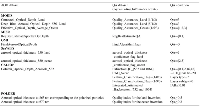
Table 2.Studied aerosol datasets, the matching data quality (QA) datasets, and the corresponding QA data screening criteria. Where provided,

numbers in parentheses in the middle column indicate the base-1 layer index, base-0 bit number, and number of bits extracted from this QA dataset. For MODIS, MISR, OMI, and SeaWiFS, the QA values are integer numbers between 0 and 3, whereas for MODIS and SeaWiFS larger numbers indicate a better retrieval quality, and for OMI and MISR the opposite is true. For POLDER, QA is a real number between 0 (worst) and 1 (best). For CALIOP, a column is accepted only if all layers found in this column meet all listed QA conditions. The listed extinction QC values indicate retrievals that are unconstrained, constrained, have a reduced lidar ratio, or detected an opaque aerosol layer. CAD score and layer type and subtype flags indicate retrievals that classified a layer with a high confidence as containing aerosol and were able to determine the aerosol type. IAB condition is set to prevent the retrieval anomaly of overcorrecting the attenuation of overlying layers (Kittaka et al., 2011).

AOD dataset QA dataset

(layer/starting bit/number of bits)

QA condition

MODIS

Corrected_Optical_Depth_Land Quality_Assurance_Land (1/1/3) QA=3

Deep_Blue_Aerosol_Optical_Depth_550_Land Quality_Assurance_Land (5/1/2) QA=3

Effective_Optical_Depth_Average_Ocean Quality_Assurance_Ocean (1/5/3) QA=[1,2,3]

MISR

RegBestEstimateSpectralOptDepth RegBestEstimateQA QA=[0,1]

OMI

FinalAerosolOpticalDepth FinalAlgorithmFlags QA=0

SeaWiFS

aerosol_optical_thickness_550_land aerosol_optical_thickness

_confidence_flag_land

QA=3

aerosol_optical_thickness_550_ocean CALIOP

aerosol_optical_thickness _confidence_flag_ocean

QA=[2,3]

Column_Optical_Depth_Aerosols_532 ExtinctionQC_[532 and 1064] QA=[0,1,2,16,18]

CAD_Score −100≤CAD<−20

Feature_Classification_Flags (1/0/3) Feature_Classification_Flags (1/9/3)

Layer type=3

Layer subtype>0 Integrated_Attenuated

_Backscatter_[532 and 1064]

IAB≤0.01

POLDER

Aerosol optical thickness at 865 nm corresponding to the polarized particles Quality index for the land inversion QA≥0.5

Aerosol optical thickness at 670 nm Quality index for the ocean inversion QA≥0.2

The MODIS (http://modis.gsfc.nasa.gov) aerosol product (MOD04 and MYD04) comprises the column aerosol optical thickness and other physical properties of aerosols retrieved globally over land and ocean (Chu et al., 2002; Hsu et al., 2004; Ichoku et al., 2005; Levy et al., 2010; Remer, 2002; Remer et al., 2005). MODIS has a swath of 2300 km.

The MISR (http://www-misr.jpl.nasa.gov) aerosol product (MIL2ASAE) features aerosol retrievals based on observa-tions from 9 independent camera angles. Though limited to a swath of 563 km, its multiple viewing angles allow MISR to measure certain aerosol properties that are not available from the other instruments (e.g., aerosol particle size). Further-more, MISR multiple cameras enable retrievals under con-ditions that are unfavorable to single-view (e.g., nadir) in-struments, such as over bright surfaces or sun glint, where the other instruments are unable to make reliable retrievals in the visible wavelengths (Kahn, 2005; Kahn et al., 2010; Martonchik et al., 2009).

The OMI (http://www.knmi.nl/omi/research/instrument/ index.php) aerosol product (OMAERUV) measures the near-UV (near ultraviolet) aerosol absorption and extinction opti-cal depth, as well as single scattering albedo, among other aerosol properties (Torres et al., 1998, 2007). In addition to offering a generous swath of 2800 km, OMI is capable of retrieving absorption optical depth in partially cloudy

con-ditions that usually pose a challenge to other aerosol instru-ments.

(6)

1

Fig. 2.Distribution of AERONET stations used in the study. Green, red, and yellow colors indicate stations that can be classified as

land-only (233 sites), ocean-land-only (11 sites), or both land-and-ocean (149 sites), respectively. The classification was established based on data availability in separate over-land and over-ocean datasets in MODIS, SeaWiFS, and POLDER aerosol products. Gray color indicates stations that do not have any collocated data for the studied period of time.

The SeaWiFS (http://disc.sci.gsfc.nasa.gov/dust/) aerosol product (SWDB) uses the Deep Blue algorithm to derive aerosol optical thickness and Ångström exponent. Also based on an orbital ground-coverage swath of 2800 km, the key fea-tures of this product are the retrievals of aerosol properties over both bright desert and vegetated surfaces, avoidance of sun glint that improves aerosol retrievals over ocean, and a highly precise calibration of the SeaWiFS sensor (Hsu et al., 2004, 2012).

The CALIOP (http://www-calipso.larc.nasa.gov) aerosol product (05kmALay) represents atmospheric curtain slices portraying the vertical distribution of aerosols and clouds in the atmosphere, including the density and certain properties of individual aerosol layers (Omar et al., 2009; Winker et al., 2007). Since CALIOP is an active lidar sensor, it can provide both daytime and nighttime retrievals within a narrow swath of about 70 m. Although the lack of the daytime background solar illumination makes nighttime CALIOP retrievals more accurate, they are not used in this study because they cannot be intercompared with the AERONET retrievals, which are available only during the daytime.

Since each of the foregoing datasets has a few versions be-cause of the periodic revisions and updates of their retrieval algorithms over time, the data versions that were current at the time of writing this paper (January 2013) were sampled, although the study has been designed in a highly flexible

way to enable rapid re-analysis as the new versions become available. The respective data versions used in this paper are AERONET AOD (Version 2), Terra and Aqua MODIS (Collection 051), MISR (Version 002), OMI (Version 003), POLDER (Versions L and K), SeaWiFS (Version 004), and CALIOP (Version 3-01). Therefore, all of the illustrations and analyses shown in this paper are based on these data ver-sions for the respective aerosol sensors.

4 Data quality screening

(7)

are identified as “bad quality” and are considered to be not trustworthy enough for certain analyses. Therefore, users of these aerosol products have been advised to choose data cor-responding to a range of QA values that is most appropriate for their specific needs.

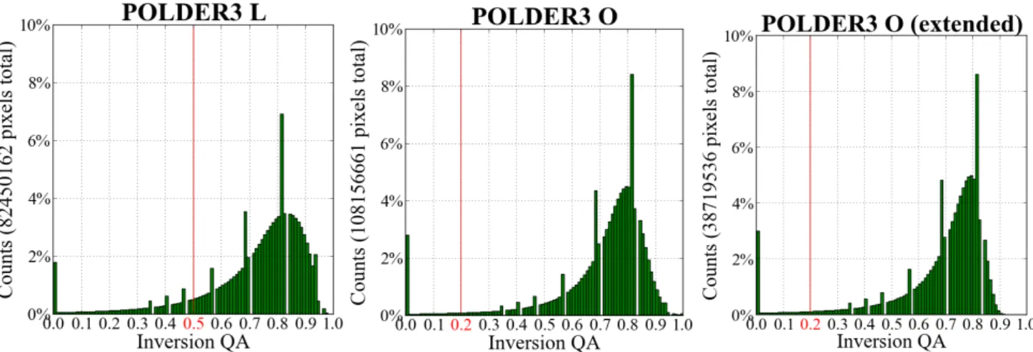
To establish similar yet valid QA thresholds for the ana-lyzed products, we consulted science teams of the anaana-lyzed products as well as data product validation results reported by these teams and other research groups. Based on this in-quiry, we chose the acceptable QA values as described in Ta-ble 2. For the majority of the products, the thresholds are set based on selecting a limited subset of the possible QA values. An important exception is the POLDER aerosol products, where the QA flags are expressed as real numbers between 0 (“bad”) and 1 (“excellent”). Since there are no formal rec-ommendations on the acceptable range of these flag values, we have adopted thresholds suggested for the “quality of in-version” flag in Bréon et al. (2011), specifically 0.5 for land retrievals and 0.2 for ocean retrievals. It is also important to note that since the primary designation of this flag is to in-dicate the success of the retrieval algorithm, this flag does not always reflect the actual quality of the retrieved aerosol parameters, especially under certain less than favorable con-ditions (Fig. 3).

The original MAPSS framework was designed to facili-tate data analysis experiments based on different values of QA flags. For this, MAPSS extracts QA flags over the sam-pling area and computes the statistical mode for integer QA flags and mean for real QA flags. These statistical modes of the integer QA flags and means of the real QA flags provide a single number for the quality assessment of each sample set, and can be used to screen the corresponding subset statistics while providing a convenient alternative compared to screen-ing individual pixels (e.g., see Levy et al., 2010; Remer et al., 2008). However, it was observed that this approach has an unequal impact on the statistical properties of the different aerosol products (Petrenko et al., 2012).

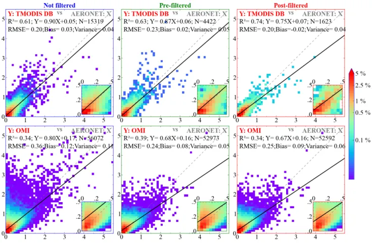
As an example, consider Fig. 4, where the global collo-cated subset mean AOD values from OMI and Terra MODIS Deep Blue (TMODIS DB) are compared to the correspond-ing subset mean AOD values from AERONET. It can be ob-served that while filtering the mean TMODIS DB AOD val-ues by the mode of QA flags improves the R2and RMSE statistics, when compared to computing the mean values based on individually screened TMODIS DB AOD pixels, this filtering significantly changes the distribution of the col-located data. Specifically, compared to screening individual pixels, QA mode filtering removes 50 % more of the collo-cated data points and degrades the slope of the fitted regres-sion line as a result of removing certain high-biased points. The opposite behavior can be observed in the collocated OMI AOD and AERONET AOD datasets, where screening by QA mode degradesR2of the collocated data when compared to screening individual pixels, although RMSE is still improved and the slope of the fitted regression line remains the same,

since both screening approaches produce approximately the same number of the OMI subset data points.

This observation indicates a certain inhomogeneity in the uncertainties that are present in the aerosol products, as in some cases high biases in individual pixels might overwhelm the statistics derived from the sample set. Therefore, to avoid such biases and ensure a fair comparison between the an-alyzed aerosol products, the rest of this study is based on the QA “pre-filtering” approach, where individual pixels in a spatial sample are screened by their QA values before com-puting the statistics of this sample. This approach also closely models a typical use of the spaceborne aerosol data, where data users screen each pixel individually and do not consider QA values of its neighboring pixels. The data quantity impact of the described QA screening approach can be observed in Table 3, which provides the sizes of the analyzed datasets before and after the screening. It is noticeable that, depend-ing on the product, the impact is quite different, with the two MODIS ocean AOD datasets and the MISR AOD dataset re-taining almost all of their available datasets, whereas the two MODIS DT datasets retained only one-fourth of the complete collocated datasets.

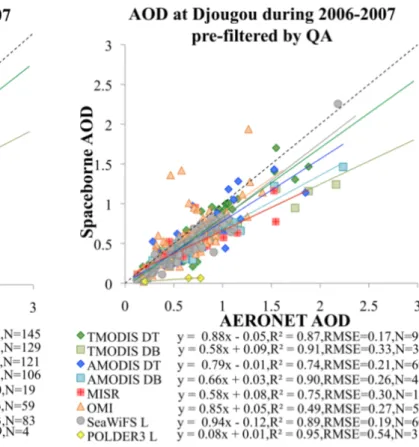
It is important however to keep in mind that the QA values reported by the retrieval algorithms are to a large degree sub-jective to these algorithms and do not always reflect the ac-tual quality of the retrievals. For example, in the absence of a proper aerosol or surface model, an algorithm can in certain cases use a wrong model to retrieve aerosol properties and mistakenly assign this retrieval a “good” QA flag (e.g., Kahn et al., 2010; Levy et al., 2010). Furthermore, a retrieval algo-rithm used might not have enough skill or even the possibility to recognize correctly certain conditions that are unfavorable for aerosol retrieval, e.g., sub-pixel cloud contamination in OMI retrievals (Torres et al., 1998). In yet another situation, an aerosol scene can be observed in only a portion of the available observation modes of a sensor, e.g., in only a few of the available observation directions in POLDER (Herman et al., 1997), which can lead to more confident yet less reli-able results. The opposite case can also be true where an al-gorithm correctly retrieves aerosol properties but is not con-fident about the retrieval. As an example, consider Fig. 5, which explores how QA screening degrades the statistics of OMI AOD and Aqua MODIS Deep Blue AOD datasets when compared to AERONET AOD over Djougou, Benin, as a sult of assigning a “bad” QA flag to sufficiently “good” re-trievals.

5 Possible data outliers

(8)

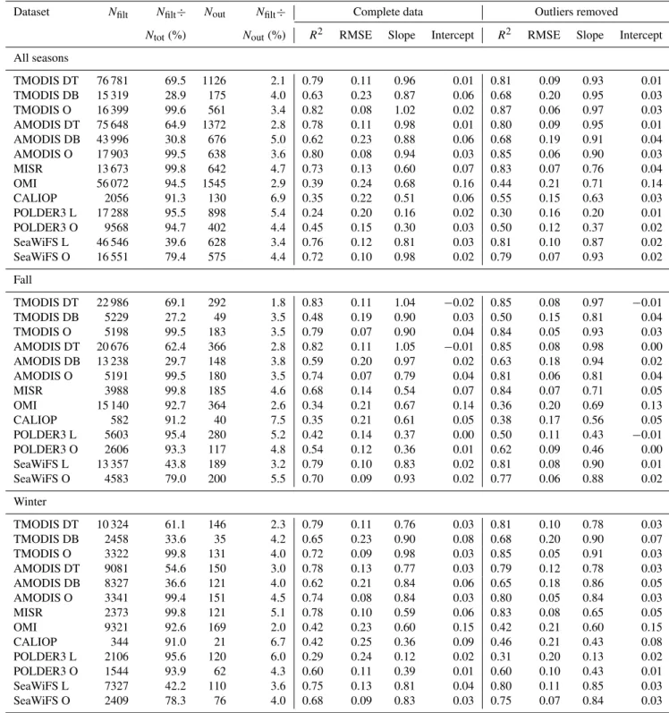
Table 3.Statistics of the studied aerosol datasets based on all AERONET stations during the period of 2006-06-07 and 2010-12-11. “Ntot”

indicates the total number of the collocated spaceborne AOD – AERONET AOD data points, while “Nfilt” indicates the number of data

points after filtering (screening) the spaceborne data by QA as described in Sect. 4 and Table 2. “Nout” is the total number of the possible

data outliers determined as explained in Sect. 5. The last 8 columns present the statistics on the collocated data based on regression fits also plotted in Fig. 6. Please see the Supplement for a breakdown of the listed statistics based on nominal ranges of AOD loading.

Dataset Nfilt Nfilt÷ Nout Nfilt÷ Complete data Outliers removed Ntot(%) Nout(%) R2 RMSE Slope Intercept R2 RMSE Slope Intercept

All seasons

TMODIS DT 76 781 69.5 1126 2.1 0.79 0.11 0.96 0.01 0.81 0.09 0.93 0.01 TMODIS DB 15 319 28.9 175 4.0 0.63 0.23 0.87 0.06 0.68 0.20 0.95 0.03 TMODIS O 16 399 99.6 561 3.4 0.82 0.08 1.02 0.02 0.87 0.06 0.97 0.03 AMODIS DT 75 648 64.9 1372 2.8 0.78 0.11 0.98 0.01 0.80 0.09 0.95 0.01 AMODIS DB 43 996 30.8 676 5.0 0.62 0.23 0.88 0.06 0.68 0.19 0.91 0.04 AMODIS O 17 903 99.5 638 3.6 0.80 0.08 0.94 0.03 0.85 0.06 0.90 0.03 MISR 13 673 99.8 642 4.7 0.73 0.13 0.60 0.07 0.83 0.07 0.76 0.04 OMI 56 072 94.5 1545 2.9 0.39 0.24 0.68 0.16 0.44 0.21 0.71 0.14 CALIOP 2056 91.3 130 6.9 0.35 0.22 0.51 0.06 0.55 0.15 0.63 0.03 POLDER3 L 17 288 95.5 898 5.4 0.24 0.20 0.16 0.02 0.30 0.16 0.20 0.01 POLDER3 O 9568 94.7 402 4.4 0.45 0.15 0.30 0.03 0.50 0.12 0.37 0.02 SeaWiFS L 46 546 39.6 628 3.4 0.76 0.12 0.81 0.03 0.81 0.10 0.87 0.02 SeaWiFS O 16 551 79.4 575 4.4 0.72 0.10 0.98 0.02 0.79 0.07 0.93 0.02 Fall

TMODIS DT 22 986 69.1 292 1.8 0.83 0.11 1.04 −0.02 0.85 0.08 0.97 −0.01

TMODIS DB 5229 27.2 49 3.5 0.48 0.19 0.90 0.03 0.50 0.15 0.81 0.04 TMODIS O 5198 99.5 183 3.5 0.79 0.07 0.90 0.04 0.84 0.05 0.93 0.03 AMODIS DT 20 676 62.4 366 2.8 0.82 0.11 1.05 −0.01 0.85 0.08 0.98 0.00

AMODIS DB 13 238 29.7 148 3.8 0.59 0.20 0.97 0.02 0.63 0.18 0.94 0.02 AMODIS O 5191 99.5 180 3.5 0.74 0.07 0.79 0.04 0.81 0.06 0.81 0.04

MISR 3988 99.8 185 4.6 0.68 0.14 0.54 0.07 0.84 0.07 0.71 0.05

OMI 15 140 92.7 364 2.6 0.34 0.21 0.67 0.14 0.36 0.20 0.69 0.13

CALIOP 582 91.2 40 7.5 0.35 0.21 0.61 0.05 0.38 0.17 0.56 0.05

POLDER3 L 5603 95.4 280 5.2 0.42 0.14 0.37 0.00 0.50 0.11 0.43 −0.01

POLDER3 O 2606 93.3 117 4.8 0.54 0.12 0.36 0.01 0.62 0.09 0.46 0.00 SeaWiFS L 13 357 43.8 189 3.2 0.79 0.10 0.83 0.02 0.81 0.08 0.90 0.01 SeaWiFS O 4583 79.0 200 5.5 0.70 0.09 0.93 0.02 0.77 0.06 0.88 0.02 Winter

TMODIS DT 10 324 61.1 146 2.3 0.79 0.11 0.76 0.03 0.81 0.10 0.78 0.03 TMODIS DB 2458 33.6 35 4.2 0.65 0.23 0.90 0.08 0.68 0.20 0.90 0.07 TMODIS O 3322 99.8 131 4.0 0.72 0.09 0.98 0.03 0.85 0.05 0.91 0.03 AMODIS DT 9081 54.6 150 3.0 0.78 0.13 0.77 0.03 0.79 0.12 0.78 0.03 AMODIS DB 8327 36.6 121 4.0 0.62 0.21 0.84 0.06 0.65 0.18 0.86 0.05 AMODIS O 3341 99.4 151 4.5 0.74 0.08 0.84 0.03 0.80 0.05 0.84 0.03

MISR 2373 99.8 121 5.1 0.78 0.10 0.59 0.06 0.83 0.08 0.65 0.05

OMI 9321 92.6 169 2.0 0.42 0.23 0.60 0.15 0.42 0.21 0.60 0.15

CALIOP 344 91.0 21 6.7 0.42 0.25 0.36 0.09 0.46 0.21 0.43 0.08

(9)

Table 3.Continued.

Dataset N_filt N_filt÷ Nout N_filt÷ Complete data Outliers removed Ntot(%) Nout(%) R2 RMSE Slope Intercept R2 RMSE Slope Intercept

Spring

TMODIS DT 15 094 70.6 207 1.9 0.80 0.11 0.92 0.03 0.81 0.10 0.94 0.02 TMODIS DB 2465 30.2 26 3.5 0.65 0.30 0.78 0.12 0.66 0.27 0.88 0.08 TMODIS O 2882 99.8 95 3.3 0.86 0.10 1.07 0.03 0.88 0.08 1.02 0.03 AMODIS DT 16 978 67.3 279 2.4 0.78 0.12 0.96 0.03 0.80 0.11 0.98 0.02 AMODIS DB 9633 32.0 88 2.9 0.63 0.27 0.83 0.09 0.66 0.25 0.89 0.07 AMODIS O 3632 99.8 142 3.9 0.81 0.09 0.99 0.03 0.86 0.07 0.94 0.04

MISR 2916 99.9 153 5.3 0.76 0.14 0.63 0.08 0.83 0.09 0.74 0.05

OMI 12 858 95.6 367 3.0 0.41 0.27 0.66 0.18 0.46 0.25 0.69 0.16

CALIOP 474 92.6 28 6.4 0.37 0.25 0.56 0.05 0.43 0.23 0.62 0.03

POLDER3 L 3766 96.3 193 5.3 0.20 0.28 0.10 0.02 0.23 0.21 0.13 0.02 POLDER3 O 2422 95.7 99 4.3 0.41 0.19 0.26 0.03 0.42 0.16 0.29 0.03 SeaWiFS L 10 512 41.7 135 3.1 0.79 0.15 0.80 0.05 0.82 0.12 0.85 0.04 SeaWiFS O 3749 79.4 118 4.0 0.73 0.12 1.04 0.01 0.78 0.08 0.97 0.02 Summer

TMODIS DT 28 377 72.3 373 1.8 0.77 0.10 1.01 0.00 0.78 0.09 1.01 0.00 TMODIS DB 5167 27.7 41 2.9 0.66 0.24 0.91 0.04 0.69 0.21 0.98 0.02 TMODIS O 4997 99.6 169 3.4 0.84 0.09 1.06 0.02 0.88 0.07 1.02 0.02 AMODIS DT 28 913 68.6 487 2.5 0.76 0.11 1.05 0.01 0.77 0.09 1.03 0.01 AMODIS DB 12 798 27.1 125 3.6 0.62 0.24 0.89 0.07 0.66 0.22 0.98 0.05 AMODIS O 5739 99.4 205 3.6 0.84 0.08 1.00 0.02 0.89 0.06 0.98 0.02

MISR 4396 99.9 219 5.0 0.72 0.13 0.62 0.08 0.82 0.08 0.79 0.04

OMI 18 753 96.1 492 2.7 0.35 0.24 0.72 0.16 0.39 0.22 0.75 0.14

CALIOP 656 90.7 30 5.0 0.34 0.18 0.54 0.05 0.49 0.14 0.64 0.02

POLDER3 L 5813 94.9 337 6.1 0.24 0.18 0.15 0.01 0.24 0.15 0.15 0.01 POLDER3 O 2996 95.5 115 4.0 0.39 0.16 0.27 0.04 0.40 0.14 0.30 0.03 SeaWiFS L 15 350 33.2 185 3.6 0.69 0.12 0.76 0.03 0.74 0.10 0.85 0.01 SeaWiFS O 5810 80.1 189 4.1 0.74 0.10 1.01 0.01 0.81 0.07 1.02 0.01

to, such factors as the lack of a proper aerosol model, in-correct assumptions about boundary conditions, cloud con-tamination, and several other factors. In Fig. 6, the possible abnormal retrievals can be visually identified by observing points that have a minimal data density and lie abnormally far from the fitted regression lines. Even though an actual fraction of such data points in a complete collocated dataset can be relatively minor, the extreme deviations of such points from the overall trend might significantly bias and misrepre-sent the overall statistics of the data. Therefore, when com-puting the overall statistics and inter-comparing the aerosol products, such data points should be treated as possible out-liers and analyzed separately from the rest of the data.

In order to identify and separate the possible data out-liers, we analyzed AOD residuals, i.e., the difference between spaceborne AOD and AERONET AOD observations, using the modified Z-score test (Iglewicz and Hoaglin, 1993; Na-tional Institute of Standards and Technology, 2012). This test is designed for testing data for multiple outliers in approxi-mately normal datasets and works by finding data points that

(10)

Fig. 3.The total quantities of POLDER3 land (“L”) and ocean (“O”) pixels based on different values of “quality of inversion” flag during

the analyzed period of July 2006–December 2010. The “POLDER3 O (extended)” histogram is based on those pixels in ocean retrievals, where the retrieval algorithm considered the sensor viewing geometry conditions to be especially “favorable” and produced a set of additional aerosol parameters, such as spherical large-mode AOD, refractive index of fine mode, and others. The quality flag values are binned into 0.01 intervals, and the red lines indicate the 0.5 (land) and 0.2 (ocean) QA thresholds used in this study. Please note that even though certain retrievals can have a very high value of inversion QA (e.g., QA > 0.9 in ocean retrievals), if they were retrieved under less than favorable conditions, they may not necessarily be high-quality aerosol data, as there are almost no extended ocean retrievals with QA > 0.9.

mostly underestimate AOD, because their retrievals focus on anthropogenic fine-mode aerosols, and thus represent only the negative portion of the distribution. In the figures, it can be seen that the distributions have long tails, strongly indicat-ing the presence of outliers. Furthermore, it can be observed that the slopes of the fitted lines are different from the slope of the 1:1 line. This indicates that the standard deviation of

the analyzed residuals is different from 1, showing that these data do not follow the standard normal distribution, although this difference does not affect the test since the modified Z-score test normalizes residuals by the median absolute devi-ation of the data.

The overall effect of removing the possible outliers can be observed in the bottom-right sub-plots of Fig. 6, Fig. 7, and Fig. 8, as highlighted by the green frames, showing that 575 (4.4 %) outliers are removed from the SeaWiFS ocean AOD dataset. The total numbers of the removed outliers are provided in Table 3 and do not exceed 7 % of the total QA-screened data for any of the datasets when considering the all-season data. The global distribution of the possible data outliers is depicted in Fig. 9 and generally corresponds to the outlier locations reported by the science teams of the aerosol products, e.g., outliers around the coastal areas where the significant subpixel surface variations, shallow waters, sed-iments, and complex marine/inland aerosol mixtures com-plicate the retrievals, and also data outliers associated with uncertain retrievals by the MODIS and MISR algorithms in Amazon Basin and near the Sahara desert (Kahn et al., 2010; Levy et al., 2010), although a more detailed study is needed to determine the specific factors that lead to these outliers and their spatiotemporal distributions. Since the Z-score test

requires the use of a reference dataset (i.e., AERONET in our case), it cannot be directly applied to remove outliers in spaceborne data in an independent and systematic fashion. However, the results of this study could possibly be used to develop appropriate mitigation measures in the retrieval al-gorithms or to design specific data screening strategies for each of the products.

In the remainder of this paper, the reported results are based on the QA-screened data with the outliers removed.

6 Analysis

The overall data distribution for the analyzed spaceborne aerosol products is presented in Fig. 6, whereas the detailed linear regression fit statistics (Fox, 1997) for the products based on the treatment of the possible data outliers and the nominal delimiters of the four boreal seasons, namely, spring (March–May), summer (June–August), autumn (September– November), and winter (December to February), are listed in Table 3. The statistics are presented based on seasonal time frames rather than monthly or shorter time periods because there may not be sufficient coincident data for a scatterplot over such shorter time periods, due to the infre-quency of satellite aerosol retrieval caused by cloud cover and other issues. Fortunately, many climatic events that are relevant to aerosol emission, transport, and distribution are often roughly aligned with these seasons.

The second column of Table 3 (Nfilt) outlines the total

(11)

1

Fig. 4.Effects of two different data QA filtering schemes on the accuracy of the global collocated spaceborne AOD, as discussed in Sect. 4.

AERONET AOD data are shown on thexaxes, while AODs measured by spaceborne sensors are on theyaxes. Density plots bin data into

0.1 AOD (0.05 AOD in magnified insets) intervals, where the color of each bin indicates the percentage of all data points that fall into this bin. Left column displays the original unfiltered data with all QA values. Middle column displays the datapre-filteredby QA, where individual

pixels in each data sample were filtered based on their QA valuesbeforecalculating the mean value of the sample. Right column shows the

datapost-filteredby QA, where the mean of each sample was calculated based on all pixels in the sample;afterthis, the whole sample was

rejected if at least half of the pixels in the sample had QA values below the specified threshold. Note that OMI data have somewhat better properties when pre-filtered, while Terra MODIS–Deep Blue data are in a better agreement with AERONET AOD when post-filtered. The insets (0–0.5 AOD range magnified) are intended to enhance the visualization of the linear regression fits near the origin.

among the main factors that determine the available vol-ume of the data (e.g., MODIS has approximately 4 times the swath width and 4 times the data volume of MISR), it can be seen that the seasonal changes in retrieval conditions also have a very considerable impact on the data. Thus, sum-mer retrievals can have 2–4 times as much collocated data points as winter retrievals. The relative data volume differ-ences between the studied data products should be carefully considered when interpreting the statistics discussed in the remainder of this paper.

In the presented statistics of Table 3, the slope value in-dicates by how much the satellite retrieval for the parameter under consideration is relatively underestimated or overes-timated across different magnitudes, depending on whether the slope value is less than or greater than unity. The offset parameter indicates the extent to which the satellite retrieval

is biased. The squared linear correlation coefficient (R2) in-dicates how consistent the parameter retrieval is across its magnitude range, that is how tightly the points are aligned close to the 1-to-1 line. Finally, the root mean square error (RMSE) indicates the accuracy of the retrievals measured as the average error in the spaceborne retrievals as compared to the ground-based AERONET retrievals.

(12)

igure 5. Impact of QA screening on the statistical properties of A

Fig. 5.Impact of QA screening on the statistical properties of AOD retrieved by the different sensors over Djougou, Benin. The top part of the

(13)

1 Figure 6. Regression fits of AERONET AOD (x-axes) to AOD

2

Fig. 6.Regression fits of AERONET AOD (xaxes) to AOD measured by spaceborne sensors (y axes). Satellite data were pre-screened

(14)

1

Fig. 7.Distribution of the difference (residuals) between spaceborne AOD and AERONET AOD. Satellite data were pre-screened by QA as

explained in Sect. 4. In each histogram, the data are split into equal-length bins of 0.05 AOD. The red vertical line indicates the residual of 0 AOD, while the blue lines mark minimum and maximum residuals of each distribution. Histogram in the green frame demonstrates the results of the possible data outlier detection and removal procedure described in Sect. 5.

same units as AOD), with the exception of MODIS Deep Blue products that have RMSE of 0.23. Removing possible outliers improves (reduces) the RMSE of all products by 13– 50 %. This indicates an opportunity for improvement of the aerosol data products by adjusting the retrieval algorithms in

the areas with the highest concentrations of the possible out-liers.

(15)

1

Fig. 8.Normality of the difference between spaceborne AOD and AERONET AOD. In each plot, points closely following the blue fitted line

indicate the data that are approximately normally distributed. Curvatures around the center of the straight line represent the departure from the normality and indicate a presence of possible outliers, particularly at the tails of the distributions. The difference in the slope and offset of the fitted blue line from the gray 1:1 line indicates a deviation from the standard location (i.e., mean=0) and scale (i.e., standard deviation =1) of the normal distribution. Satellite data were pre-screened by QA as explained in Sect. 4. Plot in the green frame demonstrates the

(16)

Fig. 9.Distribution of the possible data outliers for the studied spaceborne aerosol datasets. Displayed values are percentages from all outliers

detected for each of the datasets as listed in the fourth column of Table 3. Stations with less than 1 % from the total number of outliers are not shown. The statistical technique for detection and removal of the possible data outliers is described in Sect. 5.

the spaceborne retrieval algorithms that tend to (1) overes-timate low-AOD events when the AOD signal is very weak and almost indiscernible from the surface signal, resulting in a portion of the surface signal being mistaken for an AOD signal; and (2) underestimate high-AOD events because of the very weak surface signal, where a portion of the AOD signal might be mistaken for a surface signal. Furthermore, certain algorithms have pre-set limits on the highest possi-ble retrieved value of AOD (e.g., 3.0 in MISR), which may further affect the reported statistics. Finally, certain censors

(17)

over-0.2 0.3 0.4 0.5 0.6 0.7 0.8 0.9

Fall Winter Spring Summer

AOD R^2, based on all QA-screened data

TMODIS DT TMODIS DB TMODIS O AMODIS DT AMODIS DB AMODIS O MISR OMI CALIOP POLDER3 L POLDER3 O SeaWiFS L SeaWiFS O 0.2 0.3 0.4 0.5 0.6 0.7 0.8 0.9

AOD R^2, based on all QA-screened data with

outliers removed TMODIS DT TMODIS DB TMODIS O AMODIS DT AMODIS DB AMODIS O MISR OMI CALIOP POLDER3 L POLDER3 O SeaWiFS L SeaWiFS O 0 0.05 0.1 0.15 0.2 0.25 0.3

AOD RMSE, based on all QA-screened data TMODIS DT TMODIS DB TMODIS O AMODIS DT AMODIS DB AMODIS O MISR OMI CALIOP POLDER3 L POLDER3 O SeaWiFS L SeaWiFS O 0

0.05 0.1 0.15 0.2 0.25 0.3

Fall Winter Spring Summer AOD RMSE, based on all QA-screened data

with outliers removed

TMODIS DT TMODIS DB TMODIS O AMODIS DT AMODIS DB AMODIS O MISR OMI CALIOP POLDER3 L POLDER3 O SeaWiFS L SeaWiFS O

Fig. 10.Seasonal dependence of squared linear fit correlation coefficient (R2)and root mean square error (RMSE) statistics between the

collocated spaceborne and ground-based (AERONET) observations of AOD, based on the data in Table 3.

estimation of low-AOD events in the original Level 2 space-borne data, even when considering the associated QA infor-mation, it is especially important to explore the behavior of each product across the complete range of AOD values.

Figure 10 charts the seasonal dependence of R2 and RMSE of the spaceborne products based on the data in Ta-ble 3. While all of the products demonstrate the high seasonal variations in the statistical parameters, the OMI, CALIOP, POLDER, and MODIS Deep Blue are the most sensitive to the seasonal changes in the retrieval conditions, perhaps be-cause of the uncertainties associated with cloud screening (Li et al., 2009), although collocating spaceborne observa-tions with AERONET introduces certain bias towards cloud-free scenes because of the comprehensive AERONET cloud screening procedures (Smirnov et al., 2000). Furthermore, it can be seen that while removing the data outliers reduces the RMSE and sensitivity to the seasonal changes in the an-alyzed products, this reduction is not significant, indicating that the retrieval errors reflected by the RMSE of these prod-ucts likely stem from the regular retrievals rather than the anomalous retrievals.

The accuracy of the spaceborne aerosol products might vary with the location of the retrieval and, depending on the location, some products might be significantly more accurate than others. The spatial dependence of the accuracy of the analyzed products is explored in Fig. 11 and Fig. 12, where it can be observed that no single sensor provides the best re-trievals at all sites. Additionally, as indicated by the smaller relative sizes of certain markers in Fig. 11 and Fig. 12,

al-though some locations might be covered by highly accu-rate spaceborne retrievals from certain sensors, if such sen-sors offer limited coverage and data availability, their accu-racy advantage may ultimately produce only limited impact, highlighting the auxiliary but still important role of the less precise but more spatially extensive products. Furthermore, as depicted by the lighter shading in Fig. 11 (e.g., south-ern Australia) and also in the histogram ofR2 inset in this figure, some sites are not covered by high-correlation (i.e., R2≥0.75) retrievals at all or have no collocated retrievals from the most accurate of the products.

Moreover, it can be observed that the best-performing aerosol products differ between Fig. 11 and Fig. 12, and the products providing the best RMSE are oftentimes those with the lowerR2. Therefore, when choosing an aerosol product for a specific analysis goal and at a specific region, it is nec-essary to consider a balance between a variety of seasonal, statistical, and spatial factors.

7 Accuracy of aerosol data products based on land cover type

(18)

1

2

Fig. 11.Spaceborne datasets with the best correlation (R2)of the retrieved AOD with the AOD measured by each individual inland (top)

and coastal or island-based (bottom) AERONET site. The intensity of marker shading indicates the degree of correlation. Marker shape indicates the range of root mean square error (RMSE) associated with the displayed bestR2. Finally, marker size corresponds to the number

of collocated data points used to compute the displayed statistics. Histograms in the bottom insets highlight the distribution of these statistics over all sites based on bins of 0.05 AOD. The statistics were calculated based on the data that were pre-filtered by QA and screened of outliers as described in Sects. 4 and 5.

global dataset that is based on the International Geosphere-Biosphere Programme (IGBP) classification scheme and is available from the suite of MODIS products (Friedl et al., 2002). For each land cover type, we identified coincident AERONET stations and averaged their corresponding statis-tical results from Sect. 6. Tables 4 and 5 list the results of this aggregation, while Fig. 13 and Fig. 14 outline these results on a geographical map.

Generally, these aggregated results corroborate the find-ings of Sect. 6, and the aerosol products from MODIS and MISR sensors produce the most accurate results for the

ma-jority of the land cover types, although there are some pecu-liarities that should be discussed in greater detail in order to understand better the best areas of application of the analyzed aerosol products.

Specifically, IGBP water surface locations include 31 AERONET stations out of 160 stations with collocated ocean retrievals identified in Fig. 2. At these 31 locations, MODIS, MISR, and SeaWiFS demonstrate the best results withR2≈0.7. Furthermore, POLDER ocean dataset has a good RMSE=0.07 (Deuzé et al., 1999) that is

(19)

1

2

Fig. 12.Spaceborne datasets with the best root mean square error (RMSE) of the retrieved AOD to the AOD measured by each individual

inland (top) and coastal or island-based (bottom) AERONET site. The symbols used are the same as the symbols in Fig. 11. The statistics were calculated based on the data that were pre-filtered by QA and screened of outliers as described in Sects. 4 and 5.

has a somewhat lower squared correlation coefficient value of R2=0.62; note that these statistics are different from POLDER ocean statistics in Fig. 6, which analyzes a more complete set of AERONET stations. It is interesting to note that the correlation between AERONET and Aqua MODIS AOD withR2=0.8 is higher than the correlation between AERONET and Terra MODIS AOD withR2=0.72. A de-tailed inspection of the data showed that this difference stems from several AERONET sites with relatively small numbers of collocated data points (N <35) and the average AOD be-low 0.2. Under such be-low-AOD conditions, MODIS ocean al-gorithm has difficulty in retrieving the precise AOD values and, as a result, is subject to an increased rate of errors (Klei-dman et al., 2005; Remer, 2002).

Evergreen broadleaf forest regions provide conditions that are favorable for retrieving AOD, and multiple sensors demonstrate the high correlation with AERONET, including MODIS Dark Target withR2=0.84, MISR withR2=0.90, and POLDER withR2=0.98. However, since these regions are also susceptible to complex smoke events (e.g., Ji Parana, Brazil), sometimes combined with dust and pollution events (e.g., Anmyon, South Korea; Hong Kong, China), most of the sensors demonstrate a rather poor RMSE (Hyer et al., 2011). The important exception is POLDER dataset that has RMSE=0.07, possibly because POLDER is especially

(20)

1

Fig. 13.Land cover type dependence of squared linear fit correlation coefficient (R2) between the collocated spaceborne and ground-based

(AERONET) observations of AOD. Areas corresponding to each IGBP land cover type (bottom right inset) are colored based on the average of the data from those AERONET sites that reside in these areas. The statistics were calculated based on data that were pre-filtered by QA and screened of outliers as described in Sects. 4 and 5.

Lulin, Taiwan. It should be also noted that together with de-ciduous broadleaf forests and savannas, evergreen broadleaf forest is one of the three land cover types where POLDER demonstrates good results withR2≈0.98, indicating the ad-vantage of polarization measurements for aerosol retrievals over these regions.

Formixed forests, MODIS Dark Target products provide the highest retrieval accuracy withR2=0.78 for Terra and 0.82 for Aqua, while MISR data are somewhat less

ac-curate with R2=0.72 as a result of underestimating high AODs during summertime biomass burning events (Kahn et al., 2010), although RMSE=0.04 of MISR is better than

RMSE=0.05 of Terra MODIS and RMSE=0.06 of Aqua

MODIS. Sufficiently reliable aerosol data are also retrieved by SeaWiFS withR2=0.64, by POLDER withR2=0.62, and CALIOP withR2=0.61.

(21)

Fig. 14.Land cover type dependence of root mean square error (RMSE) between the collocated spaceborne and ground-based (AERONET)

observations of AOD. Areas corresponding to each IGBP land cover type (bottom right inset) are colored based on the average of the data from those AERONET sites that reside in these areas. The statistics were calculated based on the data that were pre-filtered by QA and screened of outliers as described in Sects. 4 and 5.

Terra andR2=0.84 for Aqua produce the best results. Al-though MODIS Deep Blue shows a better performance than MODIS Dark Target for this land cover type, the Deep Blue products are retrieved only over a single Lake Argyle AERONET site in northern Australia, whereas Dark Tar-get products are retrieved over 7 sites and have a signifi-cantly larger number of data points. Likewise, the good result demonstrated by CALIOP also originates exclusively from the Lake Argyle retrievals. The difference of 0.1 inR2 be-tween MODIS Terra Deep Blue and MODIS Aqua Deep

(22)

Fig. 15.Land cover type dependence of bias between the collocated spaceborne and ground-based (AERONET) observations of AOD. Areas

corresponding to each IGBP land cover type (bottom right inset) are colored based on the average of the data from those AERONET sites that reside in these areas. The statistics were calculated based on the data that were pre-filtered by QA and screened of outliers as described in Sects. 4 and 5.

possibly indicating the advantage of active aerosol sensing over this bright-surface region.

Overwooded savannas, both Dark Target and Deep Blue products from MODIS show very good results withR2 val-ues between 0.80 and 0.90. MISR withR2=0.79 and SeaW-iFS withR2=0.77 produce lower but still reasonably good results. The reduced performance of MISR in this region can be explained by the lack of region-specific aerosol mixtures in its retrieval algorithm, a situation that is expected to be im-proved in future revisions of the product (Kahn et al., 2009).

(23)

Fig. 16.Land cover type dependence of variance between the collocated spaceborne and ground-based (AERONET) observations of AOD.

Areas corresponding to each IGBP land cover type (bottom right inset) are colored based on the average of the data from those AERONET sites that reside in these areas. The statistics were calculated based on the data that were pre-filtered by QA and screened of outliers as described in Sects. 4 and 5.

for Terra andR2=0.61 for Aqua, MISR withR2=0.65, and MODIS Deep Blue withR2=0.52 for Terra andR2=

0.61 for Aqua, as well as CALIOP withR2=0.59.

Similar to open shrublands,grasslandswere challenging to all of the sensors, where Terra MODIS Deep Blue, Aqua MODIS Dark Target, and MISR demonstrated the best re-sults with R2 values between 0.65 and 0.67. Even more challenging weresnow and iceand alsobarren or sparsely vegetatedareas, where MISR was the only highly accurate

(24)

Table 4.Linear fit correlation coefficient (R2) between the collocated spaceborne and ground-based observations of AOD estimated at the

stations that coincide with different IGBP land cover types. Empty cells indicate no collocated data available from a specific sensor over a specific land cover type. No AERONET stations are available at the areas occupied by deciduous needleleaf forest. The statistics were calculated based on the data that were pre-filtered by QA and screened of outliers as described in Sects. 4 and 5. A graphical representation of this table is in Fig. 13. Please see the Supplement for a breakdown of the listed statistics based on the nominal boreal seasons.

TMODIS

DT

TMODIS

DB

TMODIS

O

AMODIS

DT

AMODIS

DB

AMODIS

O

MISR OMI CALIOP POLDER3

L

POLDER3

O

SeaW

iFS

L

SeaW

iFS

O

Water 0.72 0.80 0.78 0.41 0.59 0.62 0.72

Evergreen needleleaf forest 0.79 0.78 0.71 0.74 0.34 0.54 0.51 0.67 Evergreen broadleaf forest 0.84 1.00 0.84 0.90 0.60 0.14 0.98

Deciduous broadleaf forest 0.84 0.88 0.82 0.56 0.27 0.74 0.83

Mixed forests 0.78 0.82 0.72 0.39 0.61 0.62 0.64

Closed shrubland 0.51 0.74 0.64 0.84 0.90 0.50 0.88 0.55 0.60 Open shrublands 0.68 0.52 0.61 0.61 0.65 0.31 0.59 0.31 0.53 Woody savannas 0.80 0.91 0.85 0.86 0.79 0.59 0.34 0.42 0.77

Savannas 0.76 0.56 0.82 0.67 0.78 0.55 0.63 0.73 0.80

Grasslands 0.57 0.65 0.67 0.43 0.68 0.49 0.40 0.43 0.52

Permanent wetlands 0.75 0.76 0.77 0.32 0.62 0.54 0.02

Croplands 0.79 0.72 0.78 0.64 0.78 0.46 0.57 0.55 0.69

Urban and built-up 0.69 0.65 0.70 0.57 0.76 0.43 0.51 0.46 0.63 Cropland/natural veget. mosaic 0.75 0.79 0.50 0.72 0.54 0.46 0.52 0.72

Snow and ice 0.26 0.27 0.78 0.03 0.22

Barren or sparsely vegetated 0.60 0.56 0.62 0.34 0.78 0.30 0.58 0.22 0.37

Table 5.Root mean square error (RMSE) between the collocated spaceborne and ground-based observations of AOD estimated at the stations

that coincide with different IGBP land cover types. Empty cells indicate no collocated data available from a specific sensor over a specific land cover type. No AERONET stations are available at the areas occupied by deciduous needleleaf forest. The statistics were calculated based on the data that were pre-filtered by QA and screened of outliers as described in Sects. 4 and 5. A graphical representation of this table is in Fig. 14. Please see the Supplement for a breakdown of the listed statistics based on the nominal boreal seasons.

TMODIS

DT

TMODIS

DB

TMODIS

O

AMODIS

DT

AMODIS

DB

AMODIS

O

L

POLDER3

O

SeaW

iFS

L

SeaW

iFS

O

Water 0.06 0.05 0.06 0.14 0.11 0.07 0.07

Evergreen needleleaf forest 0.06 0.06 0.30 0.06 0.17 0.08 0.05 0.05 Evergreen broadleaf forest 0.09 0.80 0.08 0.10 0.28 0.59 0.07

Mixed forests 0.05 0.06 0.04 0.13 0.13 0.06 0.05

Closed shrubland 0.09 0.06 0.08 0.04 0.06 0.19 0.04 0.11 0.06 Open shrublands 0.10 0.10 0.10 0.13 0.08 0.22 0.06 0.13 0.09 Woody savannas 0.08 0.27 0.09 0.23 0.13 0.21 0.18 0.24 0.11

Savannas 0.10 0.15 0.09 0.14 0.07 0.22 0.11 0.13 0.09

Grasslands 0.09 0.18 0.09 0.16 0.05 0.19 0.11 0.13 0.08

Croplands 0.09 0.16 0.09 0.17 0.07 0.16 0.14 0.11 0.09

Urban and built-up 0.09 0.14 0.09 0.15 0.07 0.20 0.13 0.10 0.10 Cropland/natural veget. mosaic 0.07 0.08 0.13 0.06 0.15 0.22 0.08 0.11

Snow and ice 0.11 0.14 0.02 0.10 0.01

(25)

Table 6.Bias between the collocated spaceborne and ground-based observations of AOD estimated at the stations that coincide with different

IGBP land cover types. Empty cells indicate no collocated data available from a specific sensor over a specific land cover type. No AERONET stations are available at the areas occupied by Deciduous needleleaf forest. The statistics were calculated based on the data that were pre-filtered by QA and screened of outliers as described in Sects. 4 and 5. A graphical representation of this table is in Fig. 14. Please see the Supplement for a breakdown of the listed statistics based on the nominal boreal seasons.

TMODIS

DT

TMODIS

DB

TMODIS

O

AMODIS

DT

AMODIS

DB

AMODIS

O

L

POLDER3

O

SeaW

iFS

L

SeaW

iFS

O

Water 0.02 0.01 0.02 0.05 −0.04 −0.06 0.02

Evergreen needleleaf forest 0.00 0.01 0.01 0.00 0.06 −0.01 −0.05 −0.03

Evergreen broadleaf forest −0.03 0.73 0.02 −0.04 0.18 −0.47 −0.04

Deciduous broadleaf forest −0.03 −0.03 −0.01 0.02 −0.04 −0.05 −0.02

Mixed forests −0.02 0.00 0.01 0.06 0.03 −0.05 −0.02

Closed shrubland −0.01 0.00 0.02 0.02 0.03 0.11 −0.03 −0.09 −0.03

Open shrublands 0.05 0.02 0.05 0.01 0.03 0.14 −0.02 −0.11 −0.02

Woody savannas −0.04 −0.23 −0.03 −0.19 −0.08 0.03 −0.12 −0.20 −0.03

Savannas −0.05 −0.10 −0.04 −0.08 −0.02 0.08 −0.04 −0.11 −0.02

Grasslands 0.01 −0.02 0.02 0.03 0.01 0.11 −0.06 −0.11 −0.01

Permanent wetlands −0.02 0.01 0.01 0.05 −0.09 −0.05 −0.01

Croplands 0.00 0.04 0.01 −0.02 −0.03 −0.01 −0.07 −0.09 −0.04

Urban and built-up −0.01 −0.04 0.00 −0.02 −0.03 0.03 −0.05 −0.09 −0.03

Cropland/natural veget. mosaic −0.02 −0.03 0.00 −0.02 0.00 −0.02 −0.07 −0.07

Snow and ice 0.10 0.13 0.02 −0.07 0.00

Barren or sparsely vegetated 0.07 0.08 0.09 0.00 0.04 0.29 −0.01 −0.11 0.00

Table 7.Variance between the collocated spaceborne and ground-based observations of AOD estimated at the stations that coincide with

different IGBP land cover types. Empty cells indicate no collocated data available from a specific sensor over a specific land cover type. No AERONET stations are available at the areas occupied by Deciduous needleleaf forest. The statistics were calculated based on the data that were pre-filtered by QA and screened of outliers as described in Sects. 4 and 5. A graphical representation of this table is in Fig. 14. Please see the Supplement for a breakdown of the listed statistics based on the nominal boreal seasons.

TMODIS

DT

TMODIS

DB

TMODIS

O

AMODIS

DT

AMODIS

DB

AMODIS

O

L

POLDER3

O

SeaW

iFS

L

SeaW

iFS

O

Water 0.003 0.002 0.003 0.016 0.006 0.003 0.003

Evergreen needleleaf forest 0.003 0.003 0.088 0.001 0.021 0.004 0.001 0.002

Evergreen broadleaf forest 0.004 0.112 0.005 0.004 0.027 0.125 0.001

Mixed forests 0.002 0.003 0.001 0.013 0.022 0.002 0.002

Closed shrubland 0.005 0.003 0.003 0.001 0.002 0.022 0.001 0.005 0.002

Open shrublands 0.004 0.008 0.006 0.024 0.004 0.026 0.003 0.007 0.008

Woody savannas 0.004 0.020 0.004 0.014 0.019 0.024 0.017 0.027 0.014

Savannas 0.008 0.017 0.006 0.014 0.005 0.040 0.018 0.013 0.009

Grasslands 0.005 0.029 0.003 0.026 0.002 0.020 0.008 0.009 0.006

Croplands 0.006 0.027 0.007 0.028 0.005 0.021 0.022 0.005 0.006

Urban and built-up 0.006 0.015 0.007 0.016 0.004 0.030 0.011 0.004 0.007

Cropland/natural veget. mosaic 0.004 0.004 0.019 0.002 0.021 0.042 0.003 0.008

Snow and ice 0.002 0.003 0.000 0.005 0.000

(26)

8 Conclusions

In this paper, we analyzed and intercompared 11 space-borne aerosol products from MODIS, MISR, OMI, SeaW-iFS, POLDER, and CALIOP sensors, which were sampled fairly uniformly based on the MAPSS framework that was used to collocate these spaceborne observations with ground-based AERONET observations during the period of 2006-06-07 and 2010-12-11, when all the sensors were operational. Based on this analysis, for each of the AERONET stations, we identified products providing the best correlation coeffi-cient (R2)and root mean square error (RMSE). It was found that no single product provides the best retrieval over all sites, and certain sites are not covered by accurate retrievals at all. Furthermore, it was observed that a product providing the bestR2at a certain location does not always provide the best RMSE at the same location. Therefore, to facilitate the mul-tivariate analysis that is necessary when choosing the most suitable spaceborne aerosol product at a specific region, we plan to develop an interactive tool that would allow explo-ration of the multi-sensor collocated data on an interactive map.

Further, a statistical approach based on the statistical mod-ified Z-score test has been used to identify automatically pos-sible data outliers in the collocated datasets. The reported analysis shows that even though such atypical data points constitute a relatively minor portion (2–7 %) of the analyzed datasets, they can significantly bias the results of the statis-tical analysis. For this reason, it is suggested that such data points be set aside when analyzing collocated datasets and in-spected separately, in order to develop appropriate mitigation measures in the retrieval algorithms or to design specific data screening strategies that could be used to identify outliers in spaceborne datasets independently and systematically.

Finally, we assessed the accuracy of the spaceborne aerosol products based on their spatial distribution relative to different surface types derived from MODIS using the IGBP land cover classification scheme. This analysis identified sen-sors that retrieve the most accurate aerosol properties over each of the defined land cover types and highlighted the dif-ferences that exist between the sensors, providing an advan-tage or disadvanadvan-tage in retrieving AOD over a particular land cover type. Notably, some of the land cover types, including open shrublands and grasslands, had only moderately accu-rate retrievals, indicating the need for improved spaceborne aerosol remote sensing instrumentation/approaches and/or retrieval algorithms.

Supplementary material related to this article is

available online at: http://www.atmos-chem-phys.net/13/ 6777/2013/acp-13-6777-2013-supplement.pdf.

Acknowledgements. Support for the development of this project has

been provided by NASA HQ under grant number NNX08AN39A through the ROSES 2007 ACCESS Program based on a proposal entitled “Integrated validation, intercomparison, and analysis of aerosol products from multiple satellites” and also under grant NNH10ZDA001N-ESDRERR through the ROSES 2009 Earth System Data Records Uncertainty Analysis Program based on a proposal titled “Coherent uncertainty analysis of aerosol data products from multiple satellites”. We thank the science and support teams of MODIS, MISR, OMI, POLDER, CALIOP, SeaWiFS, and AERONET for retrieving and making available their respective aerosol products, as well as for providing as-sistance during the development of MAPSS sampling for these products. Specifically, we are grateful to certain individual members of the aerosol product teams for their insight and willingness to provide us answers to various questions related to their respective products, namely: AERONET (Brent Holben, Thomas Eck, Oleg Dubovik, Alexander Smirnov, David Giles), MODIS-DT (Lorraine Remer, Robert Levy, Shana Mattoo, Claire Salustro), MODIS-DB (Christina Hsu, Corey Bettenhausen, Jingfeng Huang), MISR (Ralph Kahn, Falguni Patadia, James Lim-bacher), OMI (Omar Torres, Changwoo Ahn, Suraiya Ahmad), CALIOP (David Winker, Ali Omar, Mark Vaughan), SeaWiFS (Christina Hsu, Andrew Sayer), and POLDER (Didier Tanre, Jacques Descloitres, Fabrice Ducos). We also give special thanks to the PIs of the global AERONET sites and their staff for establishing and maintaining these sites. Finally, we would like to honor the memory of our colleague, Gregory Leptoukh, who passed away suddenly in January 2012, as we had a long-term collaboration with him that resulted in the implementation of the MAPSS framework on the GIOVANNI data analysis system, and he was part of the initial discussions of the ideas that led to this study.

Edited by: M. King

References

Ahn, C., Torres, O., and Bhartia, P. K.: Comparison of Ozone Mon-itoring Instrument UV Aerosol Products with Aqua/Moderate Resolution Imaging Spectroradiometer and Multiangle Imaging Spectroradiometer observations in 2006, J. Geophys. Res., 113, D16S27, doi:10.1029/2007JD008832, 2008.

Bréon, F. M., Buriez, J. C., Couvert, P., Deschamps, P. Y., Deuzé, J. L., Herman, M., Goloub, P., Leroy, M., Lifermann, A., Moulin, C., Parol, F., Sèze, G., Tanré, D., Vanbauce, C., and Vesperini, M.: Scientific results from the Polarization and Directionality of the Earth’s Reflectances (POLDER), Adv. Space. Res., 30, 23832386, doi:10.1016/S0273-1177(02)80282-4, 2002. Bréon, F.-M., Vermeulen, A., and Descloitres, J.: An

eval-uation of satellite aerosol products against sunphotome-ter measurements, Remote Sens. Environ., 115, 3102–3111, doi:10.1016/j.rse.2011.06.017, 2011.

Cheng, T., Chen, H., Gu, X., Yu, T., Guo, J., and Guo, H.: The inter-comparison of MODIS, MISR and GOCART aerosol prod-ucts against AERONET data over China, Journal of Quan-titative Spectroscopy and Radiative Transfer, 113, 21352145, doi:10.1016/j.jqsrt.2012.06.016, 2012.