BAR, Rio de Janeiro, v. 9, n. 4, art. 3, pp. 421-440, Oct./Dec. 2012
Accrual Anomaly in the Brazilian Capital Market
César Medeiros Cupertino * E-mail address: cupertino.cmc@gmail.com Universidade Federal de Santa Catarina - UFSC
Florianópolis, SC, Brazil.
Antônio Lopo Martinez E-mail address: lopo@fucape.br Fucape Business School Vitória, ES, Brazil.
Newton Carneiro Affonso da Costa Jr. E-mail address: ncacjr@gmail.com Universidade Federal de Santa Catarina - UFSC
Florianópolis, SC, Brazil.
* Corresponding author: César Medeiros Cupertino
Abstract
This paper analyzes the phenomenon known as accrual anomaly in Brazil. In particular, we examine two hypotheses: (a) that the earnings expectation included in the stock price fails to reflect the difference in persistence of the earnings components (accruals and cash flows); and (b) that the construction of a hedge portfolio by taking a long (short) position in assets with low (high) accruals generates consistently abnormal returns. The data set includes nonfinancial firms listed on the BM&FBOVESPA between 1990 and 2008. The empirical tests required conducting panel data regressions to identify the persistence of earnings and their components; the Mishkin test to identify whether the market rationally prices earnings; and the composition of a zero-investment (hedge) portfolio to analyze whether a trading strategy based on accruals consistently provides abnormal positive returns. The results indicate that the accrual component is not mispriced by the Brazilian market, and that a trading strategy based on accruals does not provide consistently positive returns. Although this evidence does not encourage arbitrage, the results are relevant from various perspectives. The methodology applied permitted identifying the quality of earnings and of their components, as well as association between the components of earnings and returns.
Introduction
This article investigates the relationship between accruals and stock returns in the Brazilian capital market. This topic is relevant for various users of financial statements. Investment analysts follow the reported results to support their estimates or revise their forecasts. Executives often have bonuses tied to earnings, being rewarded when performance expectations are attained (executive equity compensation). Creditors use earnings as a parameter in contractual debt covenants and to monitor the borrower’s capacity to honor obligations (Smith & Warner, 1979). The focus on earnings is so intense that some authors believe the market neglects other performance measures (Chan, Chan, Jegadeesh, & Lakonishok, 2006). The fixation on earnings can carry some hidden pitfalls, mainly because of the often non-convergent interests concerning reported earnings (Jensen & Meckling, 1976).
The present article provides an expanded panorama of the relationship between accruals and stock returns in the Brazilian market. The analyses take into account specific firm characteristics (such as operational performance, risk factors and economic segment), the rationality of agents in pricing earnings and their components, and the implementation of investment strategies that seek to obtain abnormal gains from the level of accruals. The empirical tests applied to the sample permitted analyzing the phenomenon known as accrual anomaly, besides identifying the most important components of the formation, variability and persistence of the accruals of firms listed on the BMF&BOVESPA.
Our aim was to identify whether the market rationally prices earnings in the formation of expectations of future returns. The information available on the market price of assets was incorporated by applying the Mishkin test. This procedure is usually included in the studies of accrual anomaly and permits identifying possible bias between the intrinsic value of an asset and its market value. If there is asymmetry between rational valuation and market valuation, there will be an opportunity for abnormal gains by exploiting the persistence of earnings and their components.
For final verification of the occurrence of accrual anomaly in the Brazilian capital market, we constructed a zero-investment portfolio based on the magnitude of accruals. The occurrence of an anomaly is only confirmed if the zero-investment portfolio provides positive and consistent returns (Bernard, Thomas, & Wahlen, 1997). Sloan (1996) showed that a hedge strategy with a long position in assets of low accruals and a short position in assets of high accruals generates significant abnormal returns. The accrual anomaly has been intensely debated in recent international academic literature in finance (Desai, Rajgopal, & Venkatachalam, 2004; Dopuch, Seethamraju, & Xu, 2010).
However, more than a decade after publication of the seminal article by Sloan (1996), there has been no discussion of this anomaly in the Brazilian market, at least according to our search of the CAPES thesis database and Google Academic. This observation is strange since Brazil has some peculiar characteristics in relation to other countries, especially the USA. For example, Lopes and Galdi (2006, p. 28) points to the strong influence of tax rules in accounting statements in Brazil. Another aspect is international investors' strong interest in the Brazilian market.
Literature Review
Accrual anomaly
Sloan (1996) empirically identified that investors tend to overvalue accruals in forming expectations about the future earnings of U.S. firms and are surprised when the persistence of this earnings component is shorter than predicted. In the view of Defond and Park (2001), the market exaggerates in measuring accruals because investors’ expectations are biased in anticipating future reversal of this earnings component. As a consequence, companies with high (low) levels of accruals obtain negative (positive) abnormal returns, a phenomenon known as accrual anomaly. Since then, various works have examined this anomaly. Indeed, it is one of the most studied topics in recent studies of capital markets (Green, Hand, & Soliman, 2011).
This research basically has three categories of focus. One group of studies relates accrual anomaly with other anomalies, such as the works of Collins and Hribar (2000), Desai, Rajgopal and Venkatachalam (2004), and Fama and French (2008). The first work identified that accrual anomaly is different than post-earnings announcement drift (the tendency for the cumulative abnormal returns of an asset to accompany an earnings surprise for various days after its announcement, due to an overreaction of the market to the result disclosed). The second work examined accrual anomaly in the context of value glamour (the empirical regularity of firms [value companies] with low sales growth or high book-to-market, earnings-market price or cash flow-market price ratios to perform worse than firms [glamour companies] with contrary indicators). The third work found that, together with momentum (short-term returns tend to follow those observed in the recent past), accrual anomaly has the most evidence in the U.S. market.
A second group includes studies that relate abnormal returns to trading strategies based on accruals. Ali, Hwang and Trombley (2000) identified evidence contrary to the naive investor hypothesis in relation to large firms that are accompanied by analysts or held by institutional investors (the hypothesis postulates that the predictive capacity of accruals in relation to future earnings is small in these cases), and that asset price, trading volume and transaction costs do not condition the predictive capacity of accruals for future returns. Khan (2008), in turn, found that the difference in average returns of companies with very high or very low levels of accruals is explained by the difference in risk of the two types of assets.
The last category relates investors, analysts and other sophisticated users of financial statements with the properties of accruals. In this line, Bradshaw, Richardson and Sloan (2001) concluded that analysts overestimate the persistence of accruals, while Collins, Gong and Hribar (2003) found that the mispricing of accruals is reduced when there is strong institutional control. According to Lev and Nissim (2006), accrual anomaly is not eliminated in the function of systematic structural factors that prevent investors from consistently forming profitable strategies to exploit accrual anomaly, thus restricting the opportunity for arbitrage. Mashruwala, Rajgopal and Shevlin (2006) corroborated the work of Lev and Nissim (2006).
The findings of Sloan (1996) have been confirmed by other researchers, using different time periods and definitions of accruals. Among the relevant findings, there is evidence that the components of accruals, such as inventories and accounts receivable, are associated with the returns of hedge portfolios (Chan et al., 2006; Hribar, 2000; Thomas & Zhang, 2002).
respect to the legal regime, the authors argue that common law systems are more permissive (allow more flexibility) regarding accounting of accruals than are code law systems. Regarding shareholders’ rights, in countries where legal protection is weak, there is more room for managerial discretion in detriment to the interests of the shareholders (mainly the minority ones).
Ball, Kothari and Robin (2000) support the idea that the legal regime, particularly regarding the type of governance implemented, impacts accrual anomaly. In common law countries, the corporate governance system tends to be aimed at all shareholders, by intense use of financial statements and other public disclosures to mitigate problems of asymmetric information, whereas in code law countries, the governance system is oriented to the interests of the main shareholders, in a relationship of private communication (insider information). The differences of the governance system can affect the relevance of accounting information, according to the intensity with which the opportunity and conservatism resulting from the adoption of a determined legal regime reduces/increases information asymmetry, encouraging or discouraging a setting propitious for the occurrence of accrual anomaly. But there is also evidence of the presence of mispricing of accruals in countries with different legal regimes, leading to the perception that the anomaly is more reasonably explained by some systematic risk or a behavioral bias of investors in the use of accruals (LaFond, 2005, p. 11).
Accruals in Brazil
Despite the growing number of empirical works on accruals in general, research on accrual anomaly is still incipient in Brazil. Of the clusters identified in the bibliometric analysis, the most common current of investigation in the Brazilian academic literature on accruals is “earnings management”, in line with the international trend. Of the works researched on accruals, we gave greater emphasis to those listing the seminal article of Sloan in the references. When applying this criterion, it revealed another research line that relates accruals with their effect on the financial statements, particularly on distortions in the disclosed results (Colauto & Beuren, 2006, 2007).
There are also studies that examine the association of accruals and stock returns (Dantas, Medeiros, & Lustosa, 2006; Galdi & Lopes, 2009; Lopes & Galdi, 2006) and others covering the relationship between cash flows, accruals and earnings (Lustosa & Santos, 2007). In this work, the authors analyzed a sample of 92 Brazilian nonfinancial firms through time series data from 1996 to 2004 and concluded that cash flow alone is a better predictor of future flows than cash flow and accruals taken together. They also found that earnings have little informational value, a fact that urges the search for a new accounting model. Of the Brazilian works citing Sloan (1996), there are also works addressing the quality of earnings and accrual anomaly itself (Almeida, Lima, & Lima, 2009).
Methodology
Definition of variables
In this work, we used operating earnings as our earnings measure, defined as earnings before interest and taxes (EBIT). Accruals were calculated by balance sheet approach, according to Equation (1), and operating cash flows by the difference between earnings and accruals. Since accruals are calculated by the change observed between consecutive periods of the items making up working capital, there were no data available for 1990, the first year of the sample. The same situation applies to returns.
(1)
The calculation of returns required some adjustments. The time window for its measurement is one year, starting four months after the end of the previous fiscal end. This procedure is employed in other works in the Brazilian literature, such as Lopes and Galdi (2006), and in most foreign studies (Francis, Lafond, Olsson, & Schipper, 2005; Sloan, 1996; Richardson, Sloan, Soliman, & Tuna, 2005, among others). This procedure is based on the fact there is a delay between the end of the year and the date when the financial statements are published. Obtaining stock prices only at the end of the fourth month of the next year aims to assure that all the necessary information is available to construct portfolios (Fama & French, 1995) and that investors make their trading decisions under an accruals strategy at the end of April of each year of the sample. The returns (Ret) are thus calculated by:
(2a)
where is the closing price of the stock four months after the end of the fiscal year, based on the assumption that investors follow a buy-and-hold strategy until the next period.
Our definition of abnormal returns follows Sloan (1996, p. 294) and requires adjustment by the “size” variable to calculate the returns of the control portfolio. The explanatory power of the size variable for returns has been stressed in the literature (Bernard & Thomas, 1990). The returns scaled by size were calculated as the average of the excess return of individual assets over the return of a control portfolio, formed by assets of equivalent sizes, with the return given by applying a buy-and-hold strategy during the period. Specifically, the method consists of several steps. The first involves calculating the gross return of the individual assets. The next step is to identify to what control portfolio the individual asset belongs. For this, the distribution of the series is divided into quantiles by size, whose proxy is the natural logarithm of the company’s market value. Next, the return of the control portfolio is identified by the average of the gross returns of the individual assets with equivalent sizes. Formally,
∑
(2b)
where is the abnormal return of asset i in period t and ∑ is the average of the returns of the assets that compose the control portfolio. The other definitions (time window and buy-and-hold returns) are identical to those used to calculate the gross returns.
This is the method of calculating abnormal returns not only in studies of accrual anomaly (Penman & Zhang, 2002; Sloan, 1996; Xie, 2001) but also in examinations of other anomalies in the financial literature (Bernard et al., 1997).
Data and sample selection
The sample consists of all the firms listed for trading on the São Paulo Stock Exchange (BM&FBOVESPA) that are followed by Economatica. We excluded financial companies, as is common for studies in this area (Chan et al., 2006; Sloan, 1996, among others). The main reason for excluding financial firms is that they are subject to specific regulation by the Brazilian Central Bank and have specific accounting rules (Richardson, Teoh, & Wysocki, 1999), notably on the treatment of accruals (LaFond, 2005).
To avoid the influence of a small number of extreme observations (outliers), we excluded data above and below two standard deviations from the mean of the series. We also eliminated data without economic significance, probably generated by problems of the data gathered from the provider of financial information (e.g., market value or total assets less than zero). Taken together, the adjustments reduced the sample by approximately 1.8%.
Hypothesis tests
Pricing of earnings and its components (first hypothesis)
In pricing by rational expectations, investors base their decisions on the information available about all the relevant variables that affect stock returns. Using the Mishkin test enabled verification of whether stock prices reflect the difference in the persistence of the components of earnings. Mishkin (1983) established a test of market rationality and efficiency that consists of a nonlinear estimation procedure by maximum likelihood. The test was initially conceived to test the rational expectations hypothesis in macroeconomics, to supply a statistical comparison between a measure of pricing by the market (valuation coefficient) and another of rational expectations (forecasting coefficient) given by a relevant variable.
In the Mishkin test as applied by Sloan (1996), the hypothesis to be tested is that the market’s subjective expectation about stock returns is identical to the objective expectation, conditional on past information. Assuming that the model for expected return is adequately specified (i.e., the equilibrium pricing equation is correct), the parameter estimated by the model is compared with the coefficient given by an earnings regression (dependent variable) and by lagged variables (explanatory variables). If the estimate of the parameters of the two equations is different, the conclusion is that the market is not rationally using past information (i.e., the market is inefficient). For example, if the valuation coefficient is significantly higher than the forecasting coefficient, the Mishkin test indicates that the market overestimates the relevant variable (earnings and its components). The interpretation is the same (but with opposite effect) when the valuation coefficient is significantly lower than the forecasting coefficient. In this case, the market underestimates the respective variable.
The hypothesis inherent to rational expectation of future earnings states that the market’s subjective estimation is equal to the objective estimation based on the available information:
| | (3)
where
. = set of information available in period t
. | = subjective expectation of the market conditional on
. | = objective expectation conditional on
The specification given in (3) implies that the market’s expectation of earnings is equal to the true expectation conditional on all past information. Assuming the market is efficient,
| (4)
where
. = the abnormal return in period t + 1
. = the return in period t + 1
Equation (4) establishes that must not be correlated with past information. The empirical content of Equation (4) depends on a market equilibrium model, which will determine | . Abel and Mishkin (1983) provided a broad discussion of various equilibrium models
for this purpose. The market efficiency condition is:
( | ) (5)
where is the error term, is the coefficient of response of earnings and | .
Based on the earnings forecast used in Sloan (1996), the test of market rationality is based on the pricing and forecasting equations of the following system:
(6a)
(6b)
The forecasting Equation (6a) uses past information to predict future earnings. The weight given to past information, , is an objective measure of how are related to future earnings. By nonlinear estimation of the system of equations (6a) and (6b), the information on returns can be used to infer how the market uses information on to predict . Equation (3) implies that the market’s subjective expectation, conditional on past information (which can be inferred from Equation (6a)) should be equal to the objective earnings expectation, which can be estimated by Equation (6b). Therefore, the test for rationality is .
To conduct the test of equality of the coefficients, the system is estimated jointly using the nonlinear least-squares procedure. To obtain estimates of both and , it is necessary to assume that in the prediction Equation (6a) is equal to in the returns Equation (6b). In turn, if , then the sum of the squares of the residuals of the constrained estimation (SSRc), in which , should be equal to the sum of the squares of the residuals of the unconstrained estimation (SSRu), with . Mishkin (1983) showed that this restriction can be tested using the likelihood ratio test (asymptotically distributed as (q) under the null hypothesis):
(7)
where q is the number of constraints imposed when pricing is rational, n is the number of observations in each equation (2n is the number of observations in the stacked regression), is the sum of the squares of the residuals of constrained system and is the sum of the squares of the residuals of the unconstrained system.
When earnings are decomposed into operating cash flows (OCF) and accruals (Acc), the prediction and pricing equations become:
(8a)
(8b)
Here the assumption of market efficiency imposes the restrictions and , implying that the weights assigned to cash flow and accruals in the prediction equation are the same as assigned by the market to the components in the equilibrium pricing equation.
Trading strategy (second hypothesis)
Bernard, Thomas and Wahlen (1997) pointed out that an anomaly based on accounting numbers will indicate mispricing by the market only if the returns provided by a zero-investment portfolio are consistently positive. A zero-investment portfolio that produces a positive return resulting from cross-sectional differences in risk will demonstrate the variability of annual returns (Cheng & Thomas, 2006).
To verify whether a zero-investment portfolio based on accruals produces consistently positive returns in the Brazilian market, we distributed the assets by quintiles formed by the magnitude of the accruals component of earnings, resulting in the composition of five portfolios, one for each quintile (1 to 5). We repeated this procedure for each year of the sample.
In studies of accrual anomaly, this strategy is known as forming a hedge portfolio, so named because of the assumption of reduction of risk between assets with different magnitudes of the accruals component. Sloan (1996) demonstrated that such a hedge portfolio provides higher returns than maintaining a single position (long or short) based on the level of accruals.
Analysis of the Results
Descriptive statistics
Table 1 contains the descriptive statistics of the accounting variables used in the tests, divided into two panels. Panel A contains the components of working capital, and panel B contains earnings, cash flow and the components of accruals. For all the items, the annual observations were divided by the average of the total assets for the year of occurrence.
The accruals are formed by the variation of the working capital items – see Equation (1). The analysis of the working capital items provides preliminary information on the accruals, as demonstrated in panel A. Current assets are the dominant item of working capital (34% of the total assets). In turn, the accounts receivable and inventory components are the most relevant items (9.4% and 6.9% of total assets, respectively) of current assets, a similar situation to that found in international studies (Wu, Zhang, & Zhang, 2010). The current liabilities account represents 28.4% of total assets, with accounts payable (generally composed of short-term obligations to suppliers and similar creditors) being the most important item (4.6% of total assets).
Panel B contains statistics related to the variables depreciation, accruals, cash flow and variation of working capital items (third section shows details about procedures for variables’ selection). The most representative item in the formation of accruals is depreciation. However, it has small variability in relation to other items, such as Δ Accounts Receivable. According to Chan, Chan, Jegadeesh, and Lakonishok (2006), the identification of variables with greatest dispersion helps map the components that effectively permit distinguishing the accruals in the sample.
In relation to total accruals, more than half the observations are negative (median of 3.8% of total assets), indicating that the companies in general have income-decreasing accruals. The value found is very near that identified by Sloan (1996) for the U.S. market (median of 3%), and similar to the one documented by Lopes and Galdi (2006) for the Brazilian market from 1994 to 2004 (mean of
Table 1
Descriptive Statistics
Variable Mean Standard
deviation 25th percentile Median 75th percentile
A. Components of Working Capital
Current Assets 0.3725 0.2188 0.1925 0.3431 0.5306
Current Liabilities 0.3360 0.2352 0.1883 0.2841 0.4189
Accounts Receivable 0.1122 0.0893 0.0435 0.0944 0.1582
Inventories 0.0908 0.0891 0.0059 0.0686 0.1465
Other Current Assets 0.0641 0.0628 0.0232 0.0453 0.0807
Accounts Payable 0.0641 0.0615 0.0196 0.0462 0.0880
Other Current Liabilities 0.0956 0.0977 0.0380 0.0643 0.1141
B. Earnings, Cash Flow and Accruals
Δ Current Assets 0.0177 0.0795 -0.0177 0.0110 0.0524
Δ Current Liabilities 0.0139 0.0645 -0.0162 0.0077 0.0391
Depreciation 0.0417 0.0276 0.0239 0.0374 0.0558
Δ Accounts Receivable 0.0390 0.1603 -0.0304 0.0249 0.1063
Δ Inventories 0.0049 0.0303 -0.0047 0.0002 0.0145
Δ Other Current Assets 0.0049 0.0370 -0.0088 0.0027 0.0183
Δ Accounts Payable 0.0046 0.0274 -0.0065 0.0011 0.0147
Δ Other Current
Liabilities
0.0084 0.0482 -0.0105 0.0038 0.0246
Accruals -0.0397 0.0899 -0.0860 -0.0384 0.0060
Earnings 0.0414 0.0903 -0.0061 0.0443 0.0993
Cash Flow 0.0847 0.1185 0.0165 0.0866 0.1580
Note. The sample is formed of all Brazilian nonfinancial firms listed on the BM&FBOVESPA with data in the Economatica
database for the period from 1990 to 2008. Panel A presents a statistical summary of the components of working capital, while panel B offers statistics of the variation (Δ) of the nonfinancial items of current assets (Δ Current Assets –Δ Cash and Cash Equivalents), current liabilities (Δ Current Liabilities –Δ Short-term Debts –Δ Taxes Payable), accounts receivable, other current assets, accounts payable and other current liabilities. Panel B also contains the statistics depreciation, accr uals (Δ Current Assets –Δ Current Liabilities – Depreciation), earnings (operating income) and cash flow (Earnings – Accruals). The values of the variables are divided by average total assets.
Results of the hypotheses
Pricing of earnings and their components (first hypothesis)
To estimate the pricing of earnings and the respective components, we analyzed the average persistence of the following variables in future earnings: (a) current earnings, (b) cash flow and accruals. Categories (a) and (b), in turn, constitute distinct specifications under which the indicated sets of variables were tested. The results are presented in the following sub-sections. The estimates given by resolving the system composed of Equations (7a) and (7b) are shown in Table 2. The coefficient of earnings is significant both in the forecasting and the valuation equation. The estimate of the valuation equation (0.7562) is higher than that of the forecasting equation (0.6371), suggesting that the market exaggerates the effect of current earnings when estimating earnings in the following period. To find out if this effect is statistically significant, we again estimated the coefficients of Equations (6a) and (6b) imposing the constraint that . The likelihood ratio demonstrates that the null hypothesis of rational pricing cannot be rejected, indicating that the difference between the coefficients and is not significant. In panel B of Table 2, the real values of the observations were replaced by the corresponding quintiles of the distribution of the variables used in the Mishkin test. Specifically, the procedure consisted of first performing the classification by quintile for each period of the sample and then applying the Mishkin test employing this classification.
Table 2
Estimate of Pricing by the Market (Mishkin test) of Current Earnings in relation to the Implications on Earnings in the Next Period
Panel A – Regressions using real values of the variables
(6a) (6b)a.b
Forecasting coefficient Valuation coefficient
Parameter Estimate T-statistic Parameter Estimate T-statistic
0.6371 56.0530 0.7562 2.5696
Rational Pricing Test of Earnings
Likelihood Marginal
Null Hypothesis Ratio Significance
Earnings: 0.8289c 0.2895
Panel B – Regressions using classification of the variables by quantiles
Forecasting coefficient Valuation coefficient
Parameter Estimate T-statistic Parameter Estimate T-statistic
0.6363 55.41540 1.0042 2.7994
Rational Pricing Test of Earnings
Likelihood Marginal
Null hypothesis ratio significance
Earnings: 4.9059 0.0155
Note. a Equations (6a) and (6b) were estimated jointly using the iterative nonlinear least-squares method, as proposed by Mishkin (1983 as cited in Sloan, R. G. (1996). Do stock prices fully reflect information in accruals and cash flows about future earnings? Accounting Review, 71(3), 289-315). We utilized all the observations available for the period from 1990 to 2008 for nonfinancial companies with information in the Economatica database. b The earnings variable refers to earnings before interest and taxes (EBIT) divided by the average total assets. c 2N Ln(SSRc/SSRu) = 2 7.742 Ln
In panel B, the constraint imposed of equality of the rational expectations (past data) and subjective expectations (market perception) is not rejected only at a more rigorous significance of 1%. This indicates that variations within the quintile have a relevant impact on the coefficients obtained. While in panel A the hypothesis cannot be rejected that the market correctly prices earnings, in panel B the evidence is different: the market is unable to identify the impact of current earnings on future earnings. It should also be stressed that the persistence found for the effect of current earnings on earnings for the subsequent period for the Brazilian market is lower than that found for the U.S. market. For example, Sloan (1996) found a coefficient of 0.841 for the period from 1962 to 1991, and Dechow and Ge (2006) identified an estimate of 0.696 for the period from 1988 to 2002. To summarize, the Mishkin test demonstrated that the hypothesis cannot be rejected that the market rationally prices this persistence in its estimate of the implications on future earnings.
Table 3
Estimate of Pricing by the Market (Mishkin test) of the Components or Earnings in Relation to their Implications on Future Earnings
Panel A – Regressions using real values of the variables
(8a) (8b)a,b
Forecasting coefficient Valuation coefficient
Parameter Estimate T-statistic Parameter Estimate T-statistic
0.6262 52.8613 0.8333 3.3072
0.5763 38.3354 0.6523 2.0905
Rational Pricing Test of Earnings
Likelihood Marginal
Null hypothesis Ratio Significance
OCF: 3.5325 0.0363
Acc: 0.2907 0.6399
OCF, Acc: and 4.1177 0.0638
Panel B – Regressions using classification of the variables by quintiles
Forecasting coefficient Valuation coefficient
Parameter Estimate T-statistic Parameter Estimate T-statistic
0.6723 42.8437 1.0968 1.7907
0.4114 26.3778 0.2864 0.5056
Rational Pricing Test of Earnings
Likelihood Marginal
Null hypothesis ratio significance
OCF: 0.8517 0.0974
Acc: 0.0741 0.8552
OCF, Acc: and 1.7787 0.0567
Table 3 presents the estimates of the system given by Equations (8a) and (8b), related respectively to the rational pricing by past data of the components of earnings (cash flow and accruals) and the valuation by the market of the implications of the earnings components on the result of the subsequent period. Evidence indicates that the market attributes a greater weight to the persistence of cash flow (0.8333) and accruals (0.6523) than to the estimates based on past data (0.6262 for cash flow and 0.5763 for accruals). The coefficients identified were submitted to some constraints to permit additional inferences.
The data presented in panel B basically paint the same picture. The small differences are related to the valuation coefficients. The level of significance of cash flow (t = 1.7907) is smaller than that found for the regression with real data (t = 3.3072). The valuation coefficient of accruals also attracts attention, both for its magnitude (0.2864) and its statistical significance (t = 0.5056). The differences between the results presented in panels A and B corroborate the evidence discussed previously: there are fluctuations in the real values that are not captured by the standardization by quintiles. These oscillations largely result from the operational activity of the company, and in principle should not be disregarded.
Trading strategy (second hypothesis)
According to Sloan (1996), one of the ways to verify the economic significance of the results obtained by a trading strategy based on accrual anomaly is to identify the deviations of the expected returns under the hypothesis of market efficiency. Specifically, the procedure consists of forming zero-investment portfolios from assets that compose the sample, based on the magnitude of the accruals, and identifying the returns obtained by taking a long (short) position in assets with low (high) accruals and by hedging the returns of assets with extreme accruals. For our purposes here, we separated the earnings components in various ways to identify the predictive power they have for future returns. The results are presented below.
The first analysis focuses on the accruals component of earnings. The gross and abnormal returns are separated into zero-investment portfolios, with the firms grouped according to the magnitude of their accruals. If accrual anomaly occurs in the Brazilian market, the application of this strategy will enable obtaining positive abnormal returns. To corroborate the predictive power of the accruals for returns, we also present panel regressions for the firms contained in the sample.
The predictive power of earnings surprises for future returns has been evidenced in various academic works, such as Bernard and Thomas (1990) and Chan, Jegadeesh and Lakonishok (1996). A broader analysis is to include accruals in the association of earnings with returns. This focus permits verifying whether the market assigns different weights to companies that report earnings with low or high levels of accruals. This analysis is reported in Table 4.
Table 4
Returns of the Portfolios Classified by Accruals and Variation of Earnings
Accruals in relation to total assets
Δ Earnings 1 (Lowest) 2 3 4 5 (Highest) 1-5
A. Returns
1 (Lowest) 0.1454 0.0482 0.0335 0.1716 0.0078 0.1377
2 0.4426 1.0996 0.1642 0.1369 0.3522 0.0904
3 0.2213 0.2871 0.3308 0.3883 0.4498 0.2285
4 0.2910 0.3354 0.5997 0.6178 0.2733 0.0178
5 (Highest) 0.5261 0.4877 0.7053 0.6118 0.5735 0.0474
5-1 0.3807 0.4395 0.6718 0.4402 0.5657
Table 4 (continued)
Accruals in relation to total assets
Δ Earnings 1 (Lowest) 2 3 4 5 (Highest) 1-5
B. Abnormal returns
1 (Lowest) 0.2051 0.3799 0.3368 0.2322 0.3392 0.1341
2 0.0475 0.7029 0.2125 0.2458 0.0251 0.0224
3 0.2711 0.0999 0.0899 0.0514 0.0232 0.2943
4 0.0573 0.0608 0.1749 0.2043 0.1127 0.1700
5 (Highest) 0.0650 0.1121 0.3211 0.2116 0.1832 0.1182
5-1 0.2701 0.4920 0.6579 0.4438 0.5224
Note. The sample is formed of all Brazilian nonfinancial firms listed on the BM&FBOVESPA with data in the Economatica
database for the period from 1990 to 2008. The companies were classified in each year by accruals (in relation to average total assets) and independently by the variation of operating income (also in relation to average total assets). The variation of earnings is given by the difference between earnings in the reference year and those in the preceding year. The intersection of the two classifications (accruals and variation of earnings) resulted in 25 portfolios. Panel A presents the average returns (calculated by
, where P is the closing price of each stock four months after the end of the fiscal year) of the
portfolios equally weighted by quintiles of the classification variables (accruals and variation of earnings). Panel B provides the abnormal returns, calculated as the excess return over the control portfolio formed by companies of equivalent size. The classification variable for formation of the control portfolio was the natural logarithm of market value.
Panel A shows the returns, calculated by the percentage difference observed in the price of each asset between two consecutive periods. The accumulation period of the returns starts four months after the end of the year and ends four months after the end of the next year. The firms that ceased being listed during the study period because of going private or liquidation were excluded from the sample.
The returns are presented in relation to average total assets and associated with the intersection of the classifications by quintiles for accruals and variation of earnings. Therefore, the return in the first line of panel A (0.1454) represents 14.54% of the average total assets and refers to companies that had lower variation in earnings and lower level of accruals. The marginal effect of the earnings surprise (accruals) for each category of accruals (earnings surprise) is given by the spreads. The spreads were calculated by the difference between the returns of the first (last) and the last (first) quintile of the accruals (variation of earnings) and are shown in the last column (line) of panel A. The spread of the accruals for the first class of variation in earnings is positive and represents 13.77% of the total average total assets. If this behavior continued, it could be inferred that the market does a better job of pricing firms that have a lower level of accruals. However, the spread for the last class of variation in earnings (4.74%) shows that this deduction is hasty for the data in the sample.
Panel B demonstrates the results of the same procedures detailed for panel A, but in relation to abnormal returns. The adjustments in the expected return to calculate the abnormal return followed the line indicated by Sloan (1996), in which abnormal returns are identified as the buy-and-hold return of a determined asset in excess of the average buy-and-hold return of a portfolio formed of assets of equivalent size. For this purpose, the size of the firms was given by the log of equity of each firm and grouped in quintiles to calculate the average return.
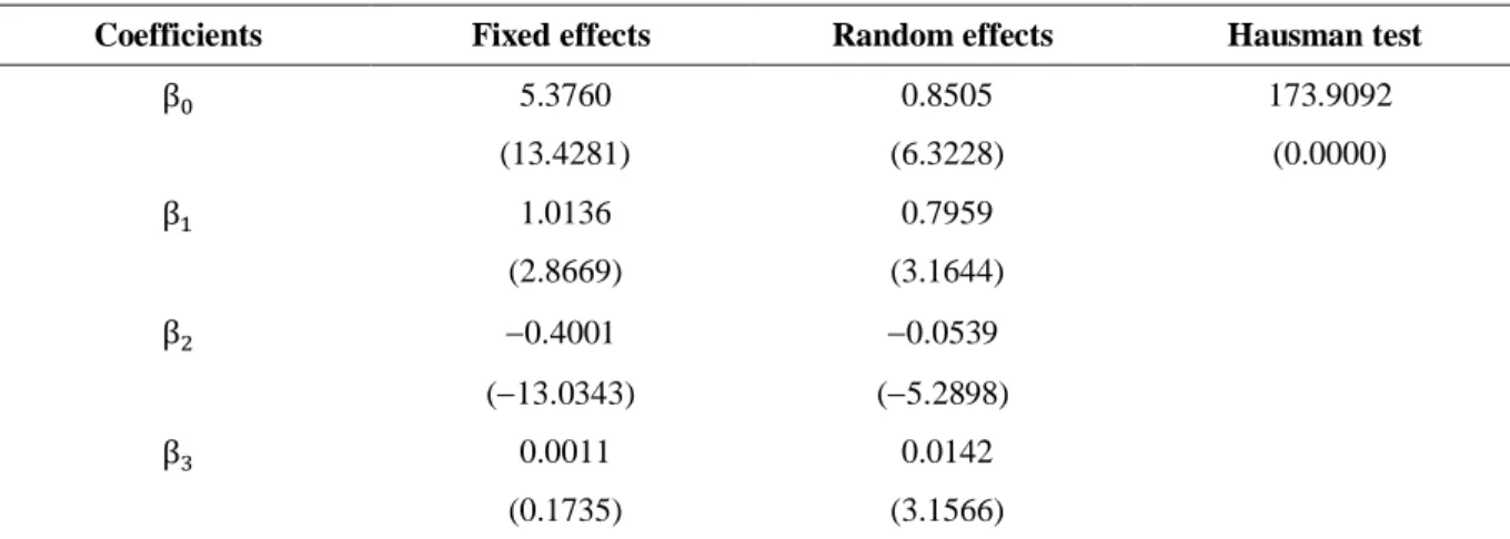
Table 5 presents the relationship between current earnings and risk proxies for future returns. The signs of the coefficients are as expected, as demonstrated in the matrix of correlations, in line with similar works (Sloan, 1996). Except for the coefficient of the book-to-market variable in the specification by fixed effects, the others are statistically significant. The regression mainly confirms that current earnings are positively related to future returns and that this relationship is significant.
Table 5
Regression of the Future Returns by Current Values of Earnings and Risk Proxies
(9)
Coefficients Fixed effects Random effects Hausman test
5.3760 0.8505 173.9092
(13.4281) (6.3228) (0.0000)
1.0136 0.7959
(2.8669) (3.1644)
0.4001 0.0539
(13.0343) (5.2898)
0.0011 0.0142
(0.1735) (3.1566)
Note. The sample is formed of all Brazilian nonfinancial firms listed on the BM&FBOVESPA with data in the Economatica
database for the period from 1990 to 2008. The returns for the next period ( ) were regressed by the current values of earnings ( ), size ( ) and book-to-market ratio ( ) in panel data for the entire time series. The t-statistic (p value) of the coefficients (Hausman test) is presented between parentheses. The returns are calculated by
(where P is
the closing price of each stock four months after the end of the fiscal year) in a buy-and-hold strategy. Size is the control variable for firm size, identified by the logarithm of the equity, and BM is the control variable given by the book-to-market ratio.
Table 6 shows the results obtained when the future returns are regressed by the components of earnings (accruals and cash flow). The coefficients obtained for the earnings components are positive and significant, indicating that for the sample chosen accruals have positive explanatory power for future returns. This finding differs from that of Sloan (1996). The institutional environment (defined as the legal regime and corporate governance practices) and some characteristics of the Brazilian capital market (such as the small number of listed companies) are some possible explanations for this divergence in the results. The Wald test does not reject the constraint imposed of equality of the coefficients of the components of earnings ( = ), indicating that the coefficients of the effect of accruals and cash flow on future returns can be considered equivalent.
Table 6
Regression of Future Returns by Current Values of Cash Flow, Accruals and Risk Proxies
(10)
Coefficients Fixed effects Random effects Hausman test
5.3052 0,8409 152,3989
(12.6443) (5,8931) (0,0000)
0.7897 0,3343
Table 6 (continued)
Coefficients Fixed effects Random effects Hausman test
(1.9295) (1,0553)
1.1936 0,7300
(3.4161) (2,9372)
0.3938 0,0528
(12.2961) (4,8881)
0.0006 0,0124
(0.0895) (2,6883)
Probability of = : 0.1414
Note. The returns in the following period ( ) were regressed by operating cash flow ( ), accruals ( ) and the control variables size and BM ratio, in panel data for the entire time series. Acc refers to accruals, obtained by focus on t he balance sheet of Equation (1). The OCF represents the difference between earnings and accruals. The other variables and sample selection procedures are as described in the note to Table 5.
When gross returns are substituted by abnormal returns in the variable to be explained, the components of earnings (accruals and cash flow) do not present statistically significant coefficients, suggesting a weak relationship between accruals and cash flow with abnormal future gains.
Table 7
Regression of Abnormal Future Returns by Current Values of Cash Flow and Accruals
(11)
Coefficients Fixed effects Random effects Hausman test
0.0364 0.0109 6.3246
(0.5333) (0.1803) (0.0423)
0.0234 0.3189
(0.0338) (0.6328)
0.4558 0.0430
(0.5630) (0.0652)
Probability of = : 0.4982
Note. The abnormal returns in the following period ( ) were regressed on the current period by the variables operating cash flow (OCF) and accruals (Acc) in panel data for the entire time series. Accruals were obtained by focus on the balance sheet of Equation (1), and OCF represents the difference between earnings and accruals. The probability of equality of the coefficients was given by the F-statistic and the Wald test. The other variables and sample selection procedures are as described in the note to Table 5.
Conclusions and Recommendations
The first hypothesis investigated establishes that the persistence of earnings and their components is mispriced by the market. To test this assumption, we applied an adaptation of Sloan (1996) to the Mishkin test. The results suggest that the market exaggerates in pricing cash flow but rationally prices the accruals component of earnings. This conclusion was submitted to some constraints to identify its robustness. Among the restrictions, the most rigorous one requires that the valuation coefficients (by the market) and forecasting coefficients (by rational expectations) be equal. In this case, we found that the hypothesis that accruals and cash flow are on average correctly priced by the market cannot be rejected.
The second hypothesis states that a hedge portfolio, based on the characteristics of accruals in the Brazilian market, consistently generates abnormal returns. We tested this hypothesis in various arrangements. In the first of these, we found that accruals do not have a marginal effect on earnings surprises. While the results of the hedge portfolio for the variation of earnings were positive and consistent, the returns related to the magnitude of accruals were unstable, fluctuating between positive and negative values. Overall, the evidence indicates that the market is somewhat efficient in pricing the variation of earnings but pays less attention to firms’ levels of accruals. These results do not correspond to those found for other countries, in that returns (including abnormal ones) are greater for firms with smaller accruals.
As an alternative procedure to the analyses based on trading strategy, the predictive power of the components of earnings for returns was identified by panel data regressions. The first of these confirmed that current earnings are positively and significantly related to future returns. When current returns were replaced by their components (accruals and cash flow), the coefficients obtained were positive and significant, indicating that for the sample chosen the accruals have positive explanatory power for future returns. This finding differs from that for the U.S. market, where this relationship has been found to be negative.
It should be pointed out that the evidence of the occurrence of accrual anomaly is modest. Besides the United States, there are only a few other countries where this anomaly has been detected, including Canada, Australia and the United Kingdom (Chan et al., 2006; Clinch, Fuller, Govendir, & Wells, 2012; LaFond, 2005; Pincus, Rajgopal, & Venkatachalam, 2007). In the Brazilian market, the evidence of accrual anomaly is not favorable to the existence of arbitrage opportunities. The empirical tests did not identify consistent and statistically significant abnormal returns, a necessary condition for such a trading strategy (based on a zero-investment portfolio) to be efficient.
In the Brazilian case, besides the findings pointed out above, this study revealed that accruals are negatively related to cash flow; that earnings management is common with the intent of decreasing the reported earnings; and that variations in the magnitude of abnormal accruals between two consecutive periods are high. The peculiarities of the Brazilian market are thus not few.
Some specific circumstances in the Brazilian capital markets and corporate reporting system, such as poor corporate governance, concentrated ownership, lack of transparency in the disclosure of accounting numbers and strong tax influence (Lopes & Galdi, 2006), may provide explanation for these results.
Received 16 November 2011; received in revised form 7 July 2012.
References
Abel, A. B., & Mishkin, F. S. (1983). An integrated view of tests of rationality, market efficiency and the short-run neutrality of monetary policy. Journal of Monetary Economics, 11(1), 3-24. doi: 10.1016/0304-3932(83)90011-9
Ali, A., Hwang, L. S., & Trombley, M. A. (2000). Accruals and future stock returns: tests of the naive investor hypothesis. Journal of Accounting, Auditing & Finance, 15(2), 161-181. doi: 10.1177/0148558X0001500204
Almeida, J., Lima, G., & Lima, I. (2009). Corporate governance and adr effects on earnings quality in the Brazilian capital markets. Corporate Ownership of Control, 7(1), 52-59.
Ball, R., Kothari, S. P., & Robin, A. (2000). The effect of institutional factors on properties of accounting earnings: international evidence. Journal of Accounting and Economics, 29(1), 1-51. doi: 10.1016/S0165-4101(00)00012-4
Bernard, V. L., Thomas, J. K., & Wahlen, J. (1997). Accounting-based stock price anomalies: separating market inefficiencies from risk. Contemporary Accounting Research, 14(2), 89-136. doi: 10.1111/j.1911-3846.1997.tb00529.x
Bernard, V. L., & Thomas, J. K. (1990). Evidence that stock prices do not fully reflect the implications of current earnings for future earnings. Journal of Accounting and Economics, 13(4), 305-340. doi: 10.1016/0165-4101(90)90008-R
Bradshaw, M. T., Richardson, S. A., & Sloan, R. G. (2001). Do analysts and auditors use information in accruals? Journal of Accounting Research, 39(1), 45-74.doi: 10.1111/1475-679X.00003
Chan, K., Chan, L. K., Jegadeesh, N., & Lakonishok, J. (2006). Earnings quality and stock returns. Journal of Business, 79(3), 1041-1082. doi: http://dx.doi.org/10.1086/500669
Chan, K., Jegadeesh, N., & Lakonishok, J. (1996). Momentum strategies. Journal of Finance, 51(5), 1681-1713. doi: 10.1111/j.1540-6261.1996.tb05222.x
Cheng, C. S., & Thomas, W. B. (2006). Evidence of the abnormal accrual anomaly incremental to operating cash flows. Accounting Review, 81(5), 1151-1167. doi: 10.2308/accr.2006.81.5.1151
Clinch, G., Fuller, D., Govendir, B., & Wells, P. (2012). The accrual anomaly: australian evidence. Accounting & Finance, 52(2), 377-394. doi: 10.1111/j.1467-629X.2010.00380.x
Colauto, R. D., & Beuren, I. M. (2006). Um estudo sobre a influência de accruals na correlação entre o earnings contábil e a variação do capital circulante líquido de empresas. Revista de Administração Contemporânea, 10(2), 95-116. doi: 10.1590/S1415-65552006000200006
Colauto, R. D., & Beuren, I. M. (2007). Análise dos reflexos do accrual accounting no earnings ou prejuízo contábil: um estudo em sociedades anônimas abertas no Brasil. BASE – Revista de Administração e Contabilidade da Unisinos, 4(2), 171-181.
Collins, D. W., & Hribar, P. (2000). Earnings-based and accrual-based market anomalies: one effect or two? Journal of Accounting and Economics, 29(1), 101-123. doi: 10.1016/S0165-4101(00)00015-X
Dantas, J. A., Medeiros, O. R., & Lustosa, P. R. (2006). Reação do mercado à alavancagem operacional: um estudo empírico no Brasil. Revista de Contabilidade & Finanças, 17(41), 72-86. doi:10.1590/S1519-70772006000200006
Dechow, P. M., & Ge, W. (2006). The persistence of earnings and cash flows and the role of special items: implications for the accrual anomaly. Review of Accounting Studies, 11(2-3), 253-296. doi: 10.1007/s11142-006-9004-1
Defond, M. L., & Park, C. W. (2001). The reversal of abnormal accruals and the market valuation of earnings surprises. Accounting Review, 76(3), 375-404.doi: 10.2308/accr.2001.76.3.375
Desai, H., Rajgopal, S., & Venkatachalam, M. (2004). Value-glamour and accruals mispricing: one anomaly or two? Accounting Review, 79(2), 355-385.doi: 10.2308/accr.2004.79.2.355
Dopuch, N., Seethamraju, C., & Xu, W. (2010). The pricing of accruals for profit and loss firms. Review of Quantitative Finance and Accounting, 34(4), 505-516. doi: 10.1007/s11156-009-0144-9
Fama, E. F., & French, K. (1995). Size and book-to-market factors in earnings and returns. Journal of Finance, 50(1), 131-155. doi: 10.1111/j.1540-6261.1995.tb05169.x
Fama, E. F., & French, K. (2008). Dissecting anomalies. Journal of Finance, 63(4), 1653-1678. doi: 10.1111/j.1540-6261.2008.01371.x
Francis, J., Lafond, R., Olsson, P., & Schipper, K. (2005). The market pricing of accruals quality. Journal of Accounting and Economics, 39(2), 295-327. doi: 10.1016/j.jacceco.2004.06.003
Galdi, F. C., & Lopes, A. B. (2009). Limits to arbitrage and value investing: evidence from Brazil [Working Paper]. Social Science Research Network. Retrieved from http://ssrn.com/ abstract=1099524
Green, J., Hand, J. R., & Soliman, M. T. (2011). Going, going, gone? The apparent demise of the accruals anomaly. Management Science, 57(5), 797-816. doi: 10.1287/mnsc.1110.1320
Hribar, P. (2000). The market pricing of components of accruals [Working Paper]. University of Iowa, Iowa City, IA, EUA.
Jensen, M. C., & Meckling, W. H. (1976). Theory of the firm: managerial behavior, agency costs and ownership structure. Journal of Financial Economics, 3(4), 305-360. doi: 10.1016/0304-405X(76)90026-X
Khan, M. (2008). Are accruals mispriced? Evidence from tests of an intertemporal capital asset pricing model. Journal of Accounting and Economics, 45(1), 55-77. doi: 10.1016/j.jacceco.2007.07.001
Lafond, R. (2005). Is the accrual anomaly a global anomaly? (Working Paper Nº 4555-05). Social Science Research Networ k. Retrieved from http://ssrn.com/paper=782726. doi: 10.2139/ssrn.782726
Lev, B., & Nissim, D. (2006). The persistence of the accruals anomaly. Contemporary Accounting Research, 23(1), 193-226. doi: 10.1506/C6WA-Y05N-0038-CXTB
Lustosa, P. R. B., & Santos, A. (2007). Poder relativo do lucro contábil e do fluxo de caixa das operações para prever fluxos de caixa futuros: um estudo empírico no Brasil. Revista de Educação e Pesquisa em Contabilidade, 1(1), 39-58.
Mashruwala, C., Rajgopal, S., & Shevlin, T. (2006). Why is the accrual anomaly not arbitraged away? The role of idiosyncratic risk and transaction costs. Journal of Accounting and Economics, 42(1-2), 3-33. doi: 10.1016/j.jacceco.2006.04.004
Mishkin, F. S. (1983). A rational expectations approach to macroeconometrics: testing policy ineffectiveness and efficient-markets models. Chicago: University of Chicago Press.
Penman, S. H., & Zhang, X. J. (2002). Accounting conservatism, the quality of earnings, and stock returns. Accounting Review, 77(2), 237-264. doi: 10.2308/accr.2002.77.2.237
Pincus, M., Rajgopal, S., & Venkatachalam, M. (2007). The accrual anomaly: international evidence. Accounting Review, 82(1), 169-203.doi: 10.2308/accr.2007.82.1.169
Richardson, S. A., Sloan, R. G., Soliman, M. T., & Tuna, I. (2005). Accrual reliability, earnings persistence and stock prices. Journal of Accounting and Economics, 39(3), 437-485. doi: 10.1016/j.jacceco.2005.04.005
Richardson, S. A., Teoh, S. H., & Wysocki, P. D. (1999). Tracking analysts’ forecasts over the annual earnings horizon: are analysts’ forecasts optimistic or pessimistic? [Working Paper]. Social Science Research Networ k. Retrieved from http://ssrn.com/paper=168191. doi: 10.2139/ssrn.168191.
Sloan, R. G. (1996). Do stock prices fully reflect information in accruals and cash flows about future earnings? Accounting Review, 71(3), 289-315.
Smith, C., & Warner, J. (1979). On financial contracting: an analysis of bond covenants. Journal of Financial Economics, 7(2), 117-161. doi: 10.1016/0304-405X(79)90011-4
Thomas, J., & Zhang, H. (2002). Inventory changes and future returns. Review of Accounting Studies, 7(2-3), 163-187.doi: 10.1023/A:1020221918065
Trammell, S. (2010). Illuminating the accruals anomaly. CFA Magazine, 21(1), 38-41. doi: 10.2469/cfm.v21.n1.7
Wu, J., Zhang, L., & Zhang, X. F. (2010). The q-theory approach to understanding the accrual anomaly. Journal of Accounting Research, 48(1), 177-223. doi: 10.1111/j.1475-679X.2009.00353.x