Rev. Bras. Econ. vol.63 número3

(1)

between Earnings and Education:

Analyzing their Evolution over Time in

Brazil

∗

Anna Crespo

†

, Mauricio Cortez Reis

‡

Contents: 1. Introduction; 2. Data; 3. Empirical Evidence; 4. Conclusion; A. Tables. Keywords: sheepskin effect; earnings; education.

JEL Code: I20; J30.

Este artigo procura analisar tendências no efeito-diploma e na relação entre rendimentos e educação no mercado de trabalho brasileiro durante o período de 1982 até 2004. Usando dados da PNAD (Pesquisa Nacional por Amostra de Domicílios) são estimadas equações de rendimentos usando, além de um termo linear para os anos de escolaridade, mudanças de in-clinação e saltos para graus completos do ciclo educacional. Também são estimadas regressões semi-paramétricas, que flexibilizam a relação entre rendimentos e educação. As evidências empíricas mostram uma redução do efeito-diploma entre 1982 e 2004, indicando que a conclusão de um grau ou a obtenção de um diploma vem perdendo valor ao longo do tempo. Ao mesmo tempo, a relação entre o logaritmo dos rendimentos e os anos de escolaridade tem se tornado mais convexa. Tendências semelhantes são verificadas quando a análise é implementada separadamente por região.

This paper seeks to analyze trends in sheepskin effects and in the relationship be-tween earnings and education on the Brazilian labor Market from 1982 to 2004. Using data from the PNAD – the Brazilian National Household Sample Survey – earnings equations are estimated including linear years of schooling, and splines and discontinuous functions for completed degrees, as well as semipara-metric regressions. Empirical evidence shows a reduction in sheepskin effects from 1982 to 2004, indicating that a diploma or degree completion in Brazil has been losing its value over time. At the same time, the relationship between log earnings and education has become more convex. Similar trends are verified when the analysis is carried out separately by region.

∗_{Os autores agradecem os comentários e sugestões de Gustavo Gonzaga e participantes do XXXIII Congresso da ANPEC. Mauricio}

Reis agradece o apoio financeiro do CNPq.

†_{Princeton University. E-mail:}_{[email protected]}

(2)

1. INTRODUCTION

There are a vast number of papers in the literature showing that earnings and education are pos-itively related (see Card (1999)). Following Mincer’s (1974) model, most of those papers represent the log of earnings as a linear function of education. Nevertheless, according to the sheepskin effect hy-pothesis, an additional year of schooling has an even stronger impact on earnings if it corresponds to a diploma or degree completion. The argument is that employers may use the information offered by a diploma or degree as a signal positively related to workers’ unobserved productivity.1 _Therefore,

sheepskin effects imply a nonlinear and discontinuous relationship between education and the log of earnings, as opposed to the standard linear earnings function established by Mincer (1974).

Evidence for different countries is consistent with the presence of sheepskin effects.2 _{In Brazil,}

esti-mates reported by Lam and Schoeni (1993) and Ramos and Vieira (1996) show that returns to schooling3

are highly nonlinear, with the completion of a degree representing a substantial earnings gain. Ramos and Vieira (1996), using PNAD data for 1990, find that an upper primary school degree (8 years of com-pleted schooling) increases earnings by 6%, and secondary school (11 years of schooling) and college (15 years of schooling) degrees increase earnings by 18%. Comparing 1976 with 1990 these authors show that sheepskin effects are very stable across time, except for the lower primary degree (4 years of schooling), which decreased slightly.

There is also a body of evidence showing that the log of earnings have become an increasingly convex function of years of schooling in the United States since 1980 (Mincer, 1974, Lemieux, 2006, Deschênes, 2006). Autor et al. (2006) argue that computerization has displaced semi-skilled workers from performing routine tasks. Since computers complement skilled workers in performing nonroutine tasks, but neither substitute nor complement unskilled workers engaged in manual tasks, changes in the earnings structure could be attributed to labor demand shifts associated with computerization. The structure of the Brazilian labor market has been changing considerably in the last decades, which could have changed the returns to education. From 1982 to 2004 the educational level of the labor force experienced a remarkable increase. In 1982 more than one third of the workers had not finished lower primary school, which requires four years of completed schooling. In 2004, this proportion decreased to about 15%. It is possible to notice also that changes in educational distribution during this period were much more intense across workers with completed degrees than for other individuals who did not have this kind of credential. These facts may have changed the signal value represented by the completion of a given degree, and then sheepskin effects are expected to lose their importance, in particular for lower degrees. A lower primary degree could be a positive signal for individual unobserved characteristics in 1982, since a great share of the workers did not reach this level of education, but probably, it offers a very different kind of information for employers in 2004.

At the same time, important changes have been occurring on the labor demand side, especially after the 1990s, when the trade liberalization process was intensified in the country and the technological progress was amplified. As documented in many papers, the technological progress should increase the relative demand for more skilled workers.4_{It is also possible that the technological progress could}

have contributed to increasing the convexity of the relationship between the log of earnings and

edu-1_{The completion of a degree could increase the signal value, since it should indicate, for example, workers’ perseverance and}

motivation, which are factors that enhance productivity (Weiss, 1995).

2_{See, for instance, Hungerford and Solon (1987), Belman and Heywood (1991), Jaeger and Page (1996) and Park (1999) for the}

United States, Ferrer and Riddell (2002) for Canada, Schady (2003) for the Philippines and Pons (2006) for Spain.

3_{It should be stressed that, although labor economists refer to the effect of an additional year of education on earnings as the}

“return to schooling”, a carefully calculation of the “return” would incorporate the tuition cost of schooling.

4_{See, for example, Berman et al. (1994) and Autor et al. (1998). Evidence from Brazil provided by Fernandes and Menezes-Filho}

(3)

cation, as in Autor et al. (2006), as well as to increasing the sheepskin effects for high level degrees and decreasing them for low level ones.

The objective of this paper is to analyze the evolution of sheepskin effects and the relationship between education and earnings in the Brazilian labor market from 1982 to 2004. In order to proceed with the empirical analysis, this paper uses data from PNAD – the Brazilian National Household Sample Survey. The empirical strategy adopted to identify the sheepskin effects consists in estimating earnings equations, including linear years of schooling, and splines and discontinuous functions for completed degrees, using demographic and labor market experience controls.

The results show that sheepskin effects represent a substantial earnings gain. Also, the patterns of sheepskin effects changed very much from 1982 to 2004, with their importance reducing over time. The lower degree, corresponding to the lower primary school, which influenced earnings in a significant way in the early 1980s, became unimportant in 2004. The effects of higher degrees also decreased from 1982 to 2004, but they are still relatively elevated in this last period. Empirical evidence also indicates a growing convexity in the relationship between education and earnings over time. Similar trends are found when the analysis is carried out separately by region.

The paper is structured as follows. The next section presents the PNAD data used in this paper, and describes educational distribution differences across periods and regions. Section 3 discusses the empirical strategy implemented in the paper. The subsequent section presents the results for the evolu-tion of sheepskin effects and the relaevolu-tionship between earnings and schooling during the last decades. Section 6 summarizes and concludes the paper.

2. DATA

This paper uses data from the 1982, 1992, 1998 and 2004 PNAD. This survey is conducted every September by the Brazilian Census Bureau (IBGE) and the sample is representative of the Brazilian population. The sample used in this paper includes workers aged 25 to 60 years, living in urban areas. All employers were excluded from the sample.

For each individual in the sample there is information about the following variables: earnings, hourly earnings, age, gender, race, region, number of years of completed schooling and potential labor market experience. This last variable is calculated using the difference between age and the age at which the worker started to work.5 _{The data contain information about 71,366 individuals in 1982;}

55,542 in 1992; 63,920 in 1998 and 83,988 individuals in 2004.

Four degrees are considered in this paper. The first degree (lower primary school) corresponds to 4 years of completed schooling. Although it had vanished during an educational system reform at the beginning of the 1970s, the first segment of primary school is included in the empirical analysis because there is a great share of workers with exactly 4 years of completed schooling, especially in older generations, and this could still be used as reference. The second degree is the upper primary school, which corresponds to 8 years of completed schooling. The next degree (secondary school) is obtained with 11 years of completed schooling, and finally, the fourth degree (college) is acquired with 15 years of completed schooling. PNAD does not distinguish between Master’s and PhD diplomas, and attributes 17 years of schooling to these degrees. Although these groups of workers are included in the sample, these degrees are not used in the paper to account for sheepskin effects. In addition, there are very few individuals with these levels of education in the sample.

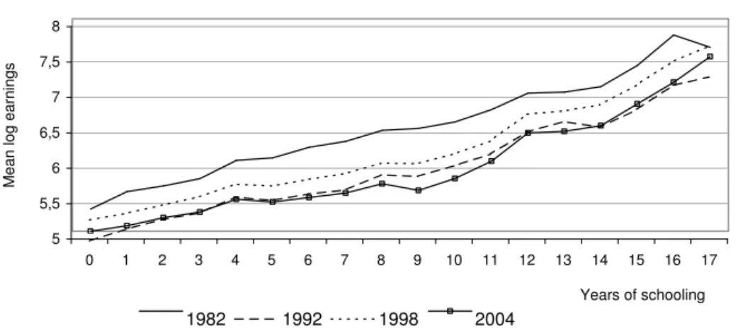
Figure 1 presents the mean log of earnings in the main job according to years of completed school-ing. From 1982 to 1992, after a period of intense macroeconomic crisis in the early 1990s, mean earnings

5_{In 1982, PNAD information about potential labor market experience was available only for the head of the household and his}

(4)

Figure 1: Mean log earnings and years of schooling

Source: Based on PNAD data for workers aged 25 to 60 years old, living in urban areas, who are the head of the household or the spouse of the head.

5 5,5 6 6,5 7 7,5 8

0 1 2 3 4 5 6 7 8 9 10 11 12 13 14 15 16 17 Years of schooling

Mean log earnings

1982 1992 1998 2004

decreased for each year of education. Mean earnings recovered in 1998 and dropped again in 2004. Fig-ure 1 shows also that the relationship between the log of earnings and education was almost linear in 1982. But it is possible to notice an increased convexity in this relationship over time. In 1982, mean earnings for workers with 10 years of schooling were around 123% higher than for those who did not complete the first year of education. In 2004, this difference fell to 75%. Mean earnings for workers with 17 years of schooling in 1982 were twice higher than those with 10 years of schooling, but in 2004 the difference between these two groups increased to 172%.

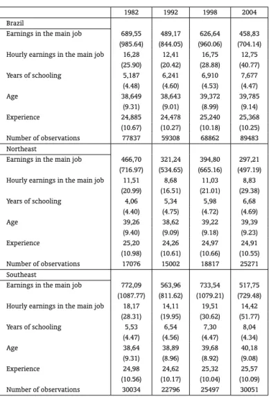
Table 1 reports the descriptive statistics for some variables for each year considered in this paper. Evidence for the total sample, in the top panel, shows that mean earnings decreased from R$ 690 in 1982 to R$ 458 in 2004. A similar trend is verified for mean hourly earnings. Average years of schooling increased from 5.2 in 1982 to 7.7 in 2004, while age and potential labor market experience increased slightly during this period.

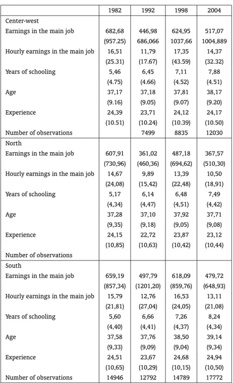
Table 1 also presents descriptive statistics comparing the Southeast and the Northeast regions. These two regions comprise around 70% of the Brazilian labor force.6The differences in mean earnings and years of schooling between the two regions are impressive. In 1982 earnings in the Southeast were 65% higher than in the Northeast, and in 2004 this ratio increased to 75%. From 1982 to 2004 the Southeast had one and a half more years of schooling than the Northeast. Table A-3 in the Appendix shows that earnings in the South and in the Center West were slightly lower than in the Southeast, while average years of schooling in the former two regions were similar to that of the Southeast. Earn-ings and average education in the North were higher than in the Northeast, but much lower than in the Southeast.

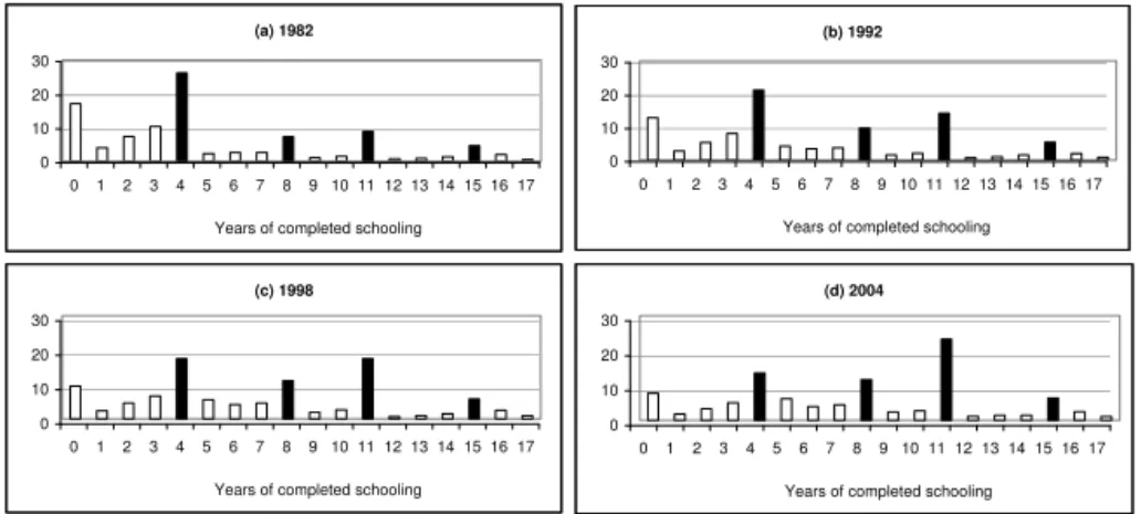
Figure 2 shows the fraction of workers in the labor force with each number of completed years of schooling in 1982, 1992, 1998 and 2002. Completed degrees are represented by dark bars. The educational level among Brazilian workers was extremely low in 1982. More than 35% of the workers had less than 4 years of completed schooling and more than 80% had less than 11 years of education. From 1982 to 2004 the educational level of the labor force increased, although it was still considerably low in 2004. The proportions with less than 4 and 11 years of schooling decreased to about 20 and 60%, respectively.

(5)

Table 1: Descriptive statistics

1982 1992 1998 2004

Brazil

Earnings in the main job 689,55 489,17 626,64 458,83

(985.64) (844.05) (960.06) (704.14)

Hourly earnings in the main job 16,28 12,41 16,75 12,75

(25.90) (20.42) (28.88) (40.77)

Years of schooling 5,187 6,241 6,910 7,677

(4.48) (4.60) (4.53) (4.47)

Age 38,649 38,643 39,372 39,785

(9.31) (9.01) (8.99) (9.14)

Experience 24,885 24,478 25,240 25,368

(10.67) (10.27) (10.18) (10.25)

Number of observations 77837 59308 68862 89483

Northeast

(716.97) (534.65) (665.16) (497.19)

(20.99) (16.51) (21.01) (29.38)

(4.40) (4.75) (4.72) (4.69)

Age 39,26 38,62 39,22 39,39

(9.40) (9.09) (9.18) (9.23)

Experience 25,20 24,26 24,97 24,91

(10.98) (10.61) (10.66) (10.55)

Southeast

(1087.77) (811.62) (1079.21) (729.48)

(28.31) (19.95) (30.62) (51.77)

(4.47) (4.56) (4.47) (4.34)

Age 38,64 38,89 39,68 40,18

(9.31) (8.96) (8.92) (9.08)

Experience 24,98 24,62 25,32 25,57

(10.56) (10.17) (10.04) (10.09)

: Notes: based on PNAD data for individuals aged 25 to 60 years old, living in urban area, who are the head of the household or the spouse of the head. Standard errors are in parenteses. Earnings in 1999 Reais.

It is interesting to notice spikes in years corresponding to completion of a degree in all periods. In 1982, the highest concentration occurred for those with a lower primary degree – near one quarter of the labor force. The proportion of workers with less than one year of education was also very high (about 17%). Seven per cent of the workers had 8 years of education in 1982, while 9% of them had 11 years of schooling. From 1982 to 2004 the change in educational distribution was mainly driven by reductions of 9 and 13 percentage points in the shares of workers with 0 and 4 years of schooling and a 15 percentage points increase in the proportion of workers with a secondary degree.

(6)

Figure 2: Educational distribution of the labor force

Source: PNAD data for workers aged 25 to 60 years old, living in urban areas, who are the head of the household or the spouse of the head.

(a) 1982

0 10 20 30

0 1 2 3 4 5 6 7 8 9 10 11 12 13 14 15 16 17 Years of completed schooling

(b) 1992

0 10 20 30

(d) 2004

0 10 20 30

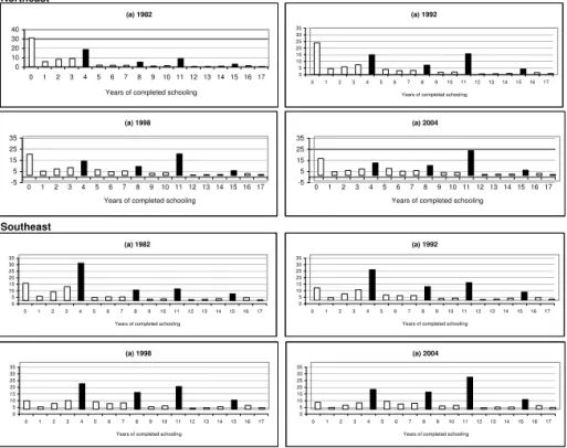
Appendix shows that changes in the South and in the North were like those verified in the Southeast, while shifts in the Center West were similar to those observed in the Northeast.

2.1. Empirical framework

In order to investigate sheepskin effects we use the standard approach adopted by Hungerford and Solon (1987) and Belman and Heywood (1991). It consists in estimating earnings equations that allow for spline functions with discontinuities in years of completed schooling corresponding to a diploma or degree completion. Spline functions may capture convexity in the relationship between earnings and education.

The dependent variable in basic regressions is the logarithm of earnings in the main job.7 Regres-sions include years of completed schooling (S), experience (Exp), experience squared (Exp2) and an interactive term between schooling and experience. The sheepskin effects are estimated by including four dummies corresponding to completed degrees. The first dummy (D4) is equal to 1 ifS ≥4, the second (D8) is equal to 1 ifS≥8, the third (D11) is equal to 1 ifS≥11and finally, there is a dummy (D15) which is equal to 1 ifS≥15. In order to allow for slope changes in the returns to the lower pri-mary school,D4is interacted with a variable equal to years of schooling minus 4. The same procedure is used for splines in upper primary, secondary and college degrees. A dummy variable for individuals with 16 years of schooling is also included. The regressions include controls for gender, race and region, represented byXi.

Belman and Heywood (1997) argue that sheepskin effects are important signals of productivity for younger cohorts, but once workers accumulate experience in the labor market, the returns to these signals decrease, because employers have more information about employees’ productivity. In order to account for this effect, the dummiesD4,D8,D11andD15are interacted with potential labor market experience.

Representing the earnings for individualibywi, the estimated specification is as follows:

7_{Regressions that use the logarithm of hourly earnings as dependent variable are reported in the Appendix and the results are}

(7)

Figure 3: Educational distribution of the labor force by region

Northeast

Southeast

Source: PNAD data for workers aged 25 to 60 years old, living in urban areas, who are the head of the household or the spouse of the head.

(a) 1982 0 10 20 30 40

(a) 1992 0 5 10 15 20 25 30 35

(a) 1998 0 5 10 15 20 25 30 35

(a) 2004 0 5 10 15 20 25 30 35

(a) 1998 -5 5 15 25 35

(a) 2004 -5 5 15 25 35

(a) 1982 0 5 10 15 20 25 30 35

(a) 1992 0 5 10 15 20 25 30 35

ln(wi) =β0+β1Si+β2Expi+β3Exp 2

i +β4Expi∗Si+β5D4i+β6D8i+β7D11i

+β8D15i+β9D4i∗(Si−4) +β10D8i∗(Si−8) +β11D11i∗(Si−11)

+β12D15i∗(Si−15) +β13S16 +β14Exp∗D4i+β15Exp∗D8i

+β16Exp∗D11i+β17Exp∗D15i+γXi+ǫi

(1)

We also estimate a more flexible specification. In this semiparametric model the log of earnings is regressed on an unrestricted set of schooling dummies:

ln(wi) =β0+ 17 X

j=1

βjSji+β18Expi+β19Exp 2

i +β20Expi∗Si+γXi+ǫi (2)

(8)

3. EMPIRICAL EVIDENCE

The estimated results are presented in two subsections. Subsection 3.1 reports the evidence for the sample of workers in Brazil. The next subsection presents evidence for the Northeast and the Southeast, comparing the results for these two regions. Regressions for other regions are shown in the Appendix.

3.1. The evolution of sheepskin effects and the earnings-education profile in the

Brazilian labor market

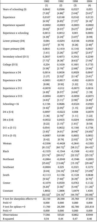
Table 2 presents the estimated results for equation (1) in 1982, 1992, 1998 and 2004. Evidence supporting sheepskin effects could be verified in all four years reported. According to Table 2, the sheepskin effects were higher for more advanced degrees, and they showed a downtrend from 1982 to 2004. The lower primary school degree increased earnings by 12% in 1982, and became nonsignificant after the 1990s.8 _{The upper primary degree effect was 12% in 1982, and increased slightly in 2004,}

when it was equal to 14%. The reductions in the coefficients for completed degrees were intense for higher credentials, but sheepskin effects were still very impressive in 2004. The secondary degree effect, which was 32% in 1982, dropped to 27% in 2004. The college degree represented an earnings increase of 31% in 1982. Twenty-two years later this effect decreased to 19%.

Changes in slope associated with a completed degree were different across periods as well. There was a drop in the spline related to lower primary school from 1982 to 2004. On the other hand, splines for secondary school and college presented an increasing trend, indicating that the reduction in sheep-skin effects was accompanied by an increase in the nonlinearity of the log of earnings returns to ed-ucation. Figure A-2 in the Appendix plots the log of the earnings-education relationship estimated in Table 2 for 1982 and 2004. The increased nonlinearity in returns to education seems very clear in this figure. F-tests reported in Table 2 indicate that sheepskin effects and spline functions related to a completed degree influence earnings in a significant way.

Table 2 also shows that interactive terms between completed degrees and experience are negative and significant in most of the regressions. So, although workers with a diploma or a degree have an extra gain in their earnings, this effect decreases with labor market experience, as predicted by Belman and Heywood (1997).

Table 3 presents the results based on semiparametric regressions for 1982, 1992, 1998 and 2004. Except for the highest level of education, it is possible to notice that estimated coefficients for each year of schooling are lower in 2004 than in 1982. This gap has an increasing trend from 1 to 10 years of education, while after 11 years the tendency is reversed. The top left graph in Figure A-3 shows the increasing convexity in the earnings-education relationship from 1982 to 2004.

Summing up, there was a reduction in the sheepskin effects from 1982 to 2004. This result could be due to the fact that the proportion of more educated workers increased over time, reducing the signal value represented by the completion of a degree. In addition, evidence shows that the relationship between earnings and education has become more convex over time.

3.2. The evolution of sheepskin effects and the earnings-education profile by

re-gion

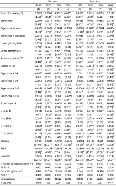
Regressions for the Northeast and the Southeast are presented in Table 4. Earnings gains associated with sheepskin effects in the Southeast have a decreasing trend over time for all degrees. Trends are not so clear in the Northeast, but indicate a reduction in sheepskin effects, too. In the Southeast as well as in the Northeast, returns to lower primary school were positive in 1982 and have become nonsignificant

8_{It is important to notice that this result could be due to the fact that lower primary education weakened part of its status}

(9)

Table 2: Earnings equation

Dependent variable: log of earnings in the main job

1982 1992 1998 2004 (1) (2) (3) (4) Years of schooling (S) 0,0659 0,0477 0,0397 0,0479

[7.05]3 [3.94]3 [3.72]3 [4.99]3 Experience 0,0176 0,0208 0,0184 0,0181 [10.10]3 _[9.41]3 _[9.71]3 _[11.05]3

Experience squared -0,0004 -0,0004 -0,0004 -0,0003 [14.06]3 _[13.33]3 _[13.15]3 _[13.24]3

Experience x schooling 0,0013 0,0015 0,001 0,0006 [4.32]3 [4.05]3 [2.94]3 [2.16]2 Lower primary (D4) 0,1158 0,0354 -0,0335 -0,034 [3.49]3 [0.81] [0.84] [0.87] Upper primary (D8) 0,1095 0,2018 0,1159 0,136 [2.67]3 [4.56]3 [3.02]3 [4.15]3 Secondary school (D11) 0,3179 0,4054 0,3138 0,2718 [6.70]3 [8.27]3 [7.75]3 [8.39]3 College (D15) 0,3106 0,2183 0,2176 0,192 [6.52]3 [3.64]3 [3.93]3 [4.29]3 Experience x D4 0 0,0017 0,0038 0,0032 [0.03] [1.14] [2.85]3 [2.48]2 Experience x D8 -0,0022 -0,0041 -0,0024 -0,0036 [1.29] [2.16]2 [1.50] [2.77]3 Experience x D11 -0,0066 -0,0118 -0,007 -0,0006 [3.78]3 _[6.49]3 _[4.75]3 _[0.55]

Experience x D15 -0,0103 -0,0085 -0,0066 -0,0068 [5.16]3 _[3.64]3 _[3.23]3 _[4.14]3

Schooling=16 0,1565 0,0666 -0,0022 -0,0418 [5.21]3 _[1.92]1 _[0.08] _[1.75]1

D4 x (S-4) -0,0019 -0,0259 0,0038 -0,0118 [0.26] [3.08]3 [0.52] [1.77]1 D8 x (S-8) -0,0058 0,0316 0,0205 -0,0031 [0.40] [2.28]2 [1.87]1 [0.33] D11 x (S-11) 0,0418 0,0628 0,0873 0,1465 [2.66]3 [3.96]3 [6.76]3 [14.01]3 D15 x (S-15) -0,0628 0,0203 0,0727 0,0954 [2.66]3 [0.87] [3.64]3 [6.09]3 Woman -0,8701 -0,7234 -0,6327 -0,5966 [120.96]3 [95.16]3 [101.62]3 [111.51]3 Black -0,1493 -0,1557 -0,1517 -0,1601 [22.22]3 [19.94]3 [22.79]3 [28.32]3 Northeast -0,3403 -0,2398 -0,2568 -0,3103 [29.82]3 _[16.17]3 _[20.41]3 _[34.44]3

Southeast -0,0238 0,2348 0,2173 0,1423 [2.29]2 _[17.36]3 _[18.09]3 _[17.23]3

South -0,1074 0,1221 0,0982 0,0726 [8.96]3 _[8.08]3 _[7.39]3 _[7.56]3

Center-west -0,1087 0,0703 0,0882 0,1437 [9.10]3 [4.58]3 [6.48]3 [14.79]3 Constant 5,7142 5,1527 5,442 5,1679 [185.57]3 [124.77]3 [150.83]3 [163.33]3 F-test for sheepskin effects=0 20,87 25,600 25,530 29,900 Prob>F 0,000 0,000 0,000 0,000 F-test for splines=0 4,51 21,680 55,030 147,180 Prob>F 0,001 0,000 0,000 0,000 Observations 71366 55542 63920 83988 R-squared 0,54 0,46 0,50 0,48 a_{Note: Robust t-statistics in brackets.}

1_{Significant at 10%.}

2_{Significant at 5%.}

(10)

Table 3: Earnings equation – semiparametric approach

1982 1992 1998 2004

(1) (2) (3) (4)

Years of schooling=1 0,1301 0,1072 0,0529 0,0519

[7.88]3 [4.49]3 [2.39]2 [2.48]2

[15.10]3 [10.02]3 [6.59]3 [6.07]3

[20.42]3 _[14.14]3 _[11.56]3 _[10.57]3

[37.02]3 [25.96]3 [20.99]3 [20.08]3

[23.61]3 [18.63]3 [18.04]3 [17.43]3

[27.23]3 _[20.85]3 _[19.63]3 _[18.18]3

[30.33]3 _[21.70]3 _[21.90]3 _[19.97]3

[41.75]3 [30.39]3 [28.58]3 [25.81]3

[27.02]3 _[23.28]3 _[24.44]3 _[20.10]3

[32.68]3 _[26.79]3 _[25.87]3 _[23.41]3

[53.74]3 [39.75]3 [40.31]3 [39.03]3

[35.31]3 _[29.54]3 _[29.41]3 _[39.63]3

[38.18]3 _[33.54]3 _[34.05]3 _[40.53]3

[47.16]3 [35.32]3 [38.96]3 [41.50]3

[61.22]3 [48.05]3 [53.56]3 [57.59]3

[59.89]3 _[45.37]3 _[53.46]3 _[57.40]3

[39.46]3 [38.90]3 [48.76]3 [57.61]3

Constant 5,609 4,9041 5,2281 5,0254

[201.85]3 [149.41]3 [185.03]3 [202.03]3

Observations 71366 64342 74335 98414

R-squared 0,54 0,44 0,48 0,46

Note: Robust t-statistics in brackets.

Regressions control for potencial experience, potencial experience squared, gender, race, region and years of schooling x potencial experience.

1_{significant at 10%.}

2

significant at 5%.

(11)

Table 4: Earnings equation

Northeast Southeast 1982 1992 1998 2004 1982 1992 1998 2004

(1) (2) (3) (4) (5) (6) (7) (8) Years of schooling (S) 0,0823 0,0668 0,0647 0,0561 0,0488 0,0441 0,0063 0,0163

[4.10]3 [2.54]2 [3.10]3 [2.88]3 [3.47]3 [2.32]2 [0.36] [1.03] Experience 0,0091 0,0173 0,0215 0,0136 0,0216 0,023 0,0182 0,0196 [2.47]2 [3.71]3 [5.82]3 [4.05]3 [8.17]3 [6.71]3 [5.94]3 [7.35]3 Experience squared -0,0002 -0,0004 -0,0004 -0,0003 -0,0005 -0,0005 -0,0004 -0,0004 [4.18]3 [4.71]3 [7.05]3 [4.97]3 [11.41]3 [10.13]3 [8.79]3 [9.23]3 Experience x schooling 0,0014 0,0012 0,0006 0,001 0,0015 0,0012 0,0011 0,0005 [1.99]2 _[1.33] _[0.92] _[1.68]* _[3.26]3 _[2.17]2 _[2.10]2 _[1.03]

Lower primary (D4) 0,1339 0,0244 0,0129 0,009 0,1259 -0,0255 -0,0429 -0,0338 [1.72]1 _[0.22] _[0.15] _[0.11] _[2.62]3 _[0.39] _[0.69] _[0.54]

Upper primary (D8) -0,1467 0,2977 0,0941 0,0217 0,2129 0,1222 0,1284 0,1447 [1.49] [2.85]3 [1.14] [0.30] [3.54]3 [1.81]1 [2.13]2 [2.78]3 Secondary school (D11) 0,4276 0,4712 0,27 0,3389 0,2694 0,33 0,3076 0,2722 [3.81]3 [4.15]3 [3.27]3 [4.88]3 [3.76]3 [4.25]3 [4.67]3 [5.16]3 College (D15) 0,1138 -0,0083 0,2673 0,1664 0,3392 0,2512 0,1585 0,1869 [0.97] [0.05] [2.10]2 [1.71]1 [4.93]3 [2.80]3 [1.91]1 [2.61]3 Experience x D4 -0,0025 0,004 0,0016 0,0006 0,001 0,0038 0,0052 0,0048 [0.84] [1.03] [0.52] [0.22] [0.57] [1.77]1 [2.52]2 [2.40]2 Experience x D8 0,0062 -0,0056 -0,0016 -0,0024 -0,0055 -0,0022 -0,0037 -0,0038 [1.53] [1.25] [0.47] [0.80] [2.24]2 [0.77] [1.47] [1.87]1 Experience x D11 -0,0119 -0,0063 -0,0018 -0,0008 -0,0049 -0,0116 -0,0076 -0,0008 [2.94]3 [1.53] [0.61] [0.32] [1.94]1 [4.16]3 [3.18]3 [0.45] Experience x D15 -0,0108 -0,0083 -0,006 -0,0099 -0,0114 -0,0091 -0,0052 -0,005 [2.30]2 [1.51] [1.34] [2.66]3 [4.09]3 [2.65]3 [1.65]1 [1.97]2 Schooling=16 0,1692 0,0177 0,0474 0,1496 0,1887 0,0895 0,0091 -0,0984 [2.46]2 _[0.22] _[0.72] _[2.69]3 _[4.31]3 _[1.73]1 _[0.22] _[2.70]3

D4 x (S-4) -0,0115 -0,0517 -0,0197 0,0005 0,0091 -0,0106 0,0387 0,0218 [0.67] [2.56]2 _[1.29] _[0.03] _[0.88] _[0.83] _[3.35]3 _[2.05]2

D8 x (S-8) 0,0037 0,0062 0,0288 -0,0285 -0,0047 0,0339 0,0087 -0,0051 [0.10] [0.17] [1.13] [1.35] [0.22] [1.59] [0.51] [0.34] D11 x (S-11) 0,1224 0,1907 0,0961 0,186 0,0264 0,0497 0,0992 0,1383 [3.09]3 [4.41]3 [2.99]3 [7.89]3 [1.14] [2.06]2 [5.10]3 [8.37]3 D15 x (S-15) -0,1139 -0,045 0,0748 0,0487 -0,0633 0,0104 0,0751 0,1028 [2.07]2 [0.79] [1.67]* [1.27] [1.79]1 [0.31] [2.58]3 [4.39]3 Woman -0,9434 -0,7884 -0,6397 -0,6045 -0,8758 -0,7199 -0,626 -0,6025 [57.08]3 [43.31]3[48.47]3[50.01]3 [84.46]3 [64.26]3[64.86]3 [72.22]3 Black -0,0808 -0,1278 -0,1085 -0,125 -0,1806 -0,1744 -0,1744 -0,1832 [5.38]3 [6.97]3 [7.54]3 [9.94]3 [19.12]3 [15.92]3[18.00]3 [21.89]3 Constant 5,4246 4,8625 5,0393 4,7956 5,6883 5,4416 5,7818 5,4132 [92.16]3 [64.27]3[81.68]3[81.76]3 [123.78]3[85.29]3[99.99]3[101.94]3 F-test for sheepskin effects=0 4,920 6,860 4,230 7,330 10,220 8,460 9,350 11,330 Prob>F 0,001 0,000 0,002 0,000 0,000 0,000 0,000 0,000 F-test for splines=0 6,620 11,030 11,040 30,920 1,640 8,210 34,120 65,370 Prob>F 0,000 0,000 0,000 0,000 0,162 0,000 0,000 0,000 Observations 15402 13361 16512 22391 27592 21051 22809 26957 R-squared 0,50 0,4 0,44 0,41 0,53 0,44 0,47 0,47

Note: Robust t-statistics in brackets. 1

significant at 10%. 2_{significant at 5%.}

(12)

thereafter. The same pattern is verified for upper primary education in the Southeast. The coefficient associated with secondary school decreased in the Northeast and remained almost constant in the Southeast. The college degree coefficient was nonsignificant in 1982 and 1992 in the Northeast and became positive and significant in 1998 and 2004. In the Southeast, the extra earnings gain associated with the completion of college present a decreasing trend, but they were still very high in 2004 (19%). F-tests show that the sheepskin effect coefficients were significantly different from zero in all regressions reported. It is possible to notice in Table 4 that each additional year of schooling has a stronger impact on the log of earnings in the Northeast than in the Southeast. These linear effects decreased from 1982 to 2004 in both regions.

According to Table 4, a positive trend over time is verified for the spline associated with college degree only for the Southeast, while spline functions related to secondary school present an increasing trend in both regions. F-tests for spline functions are significant in all cases, except for the Southeast in 1982. These changes in spline functions imply a growing convexity of the log of the earnings-schooling relationship, which is more dramatic for the Southeast, as shown in Figure A-2. Evidence from semiparametric regressions is presented in Figure A-3. Returns to schooling seem to be an even more convex function of years of education using this specification.

Evidence provided by Lemieux (2006) shows that since the 1980s log earnings have become an increasingly convex function of years of schooling in the United States. According to Autor et al. (2006), these changes could be explained by the intensive use of computers, which complements non-routine and more complex tasks of highly educated workers and substitutes the routine tasks performed by workers in the middle of the educational distribution. Computers may have lower consequences for non-routine manual tasks of less educated individuals. Our evidence reported in Figure A-2 is consistent with the argument of Autor et al. (2006). The reduction in mean labor earnings from 1982 to 2004 was much more intense for middle-educated workers with years of schooling between 4 and 10, mainly in the Southeast, when compared to the Northeast.

The Appendix reports evidence for the other three Brazilian regions. In each one of these cases sheepskin effects also present a negative trend over time. In addition, it is possible to notice that spline functions for high degrees have the same positive trend verified for the whole country. Growing convexity in the log of the earnings-education relationship was identified for the South and the Center West in Figure A-2, which uses splines and discontinuous functions, as well as for the former region in Figure A-3 using dummies for years of schooling.

4. CONCLUSION

This paper is concerned with analyzing the evolution of sheepskin effects in Brazil from 1982 to 2004. During this period, a lot of changes occurred in the Brazilian labor market, which could be connected with alterations in the relationship between earnings and schooling. On the one hand, there was a substantial increase in the supply of more educated individuals. On the other hand, firms increased the necessity of hiring high skilled workers as they adopted new technologies, especially after the 1990s.

The results estimated using PNAD data show that sheepskin effects changed considerably during the period analyzed, as well as did the relationship between education and log earnings. From 1982 to 2004, the sheepskin effect basically disappeared for the first degree (lower primary school), and decreased for secondary and college degrees. This evidence is consistent with the higher supply of more educated workers in the labor force reducing the importance of higher degrees as a signal of more productive workers. However, estimated earnings gains associated with the completion of these degrees were still elevated in 2004.

(13)

was more dramatic for middle-educated workers, who had between 4 and 10 years of completed school-ing. For those with very low educational level or with more than 12 years of schooling the reductions in earnings were not so strong.

The results by region show that growing convexity of the relationship between the log of earnings and education were more intense in the Southeast, South and Center West. In addition, we found reductions in the sheepskin effects over time in each one of the Brazilian regions separately.

BIBLIOGRAPHY

Autor, D., Katz, L., & Kearney, M. (2006). The polarization of the U.S. labor market. mimeo.

Autor, D., Katz, L., & Krueger, A. (1998). Computing inequality: Have computers changed the labor market? Quarterly Journal of Economics, 113(4).

Belman, D. & Heywood, J. (1991). Sheepskin effects in return to education: An examination of women and minorities. Review of Economics and Statistics, 73:720–724.

Belman, D. & Heywood, J. (1997). Sheepskin effects by Cohorts: Implications of job matching in a signaling model.Oxford Economic Papers, 49(4):623–637.

Berman, E., Bound, J., & Griliches, Z. (1994). Changes in the demand for skilled labor within U. S. manufacturing industries: Evidence from the annual survey of manufactures. Quarterly Journal of Economics, 109(2).

Card, D. (1999). The casual effect of education on earnings. In Ashenfelter, O. & Card, D., editors,

Handbook of Labor Economics, Vol.

Deschênes, O. (2006). Unobserved ability, comparative advantage, and the rising return to education in the United States 1979-2002. mimeo.

Fernandes, R. & Menezes-Filho, N. (2002). Escolaridade e demanda relativa por trabalho. InO Mercado de Trabalho No Brasil. LTR, São Paulo.Menezes-Filho, N. & Chahad, J.

Ferrer, A. & Riddell, W. (2002). The role credentials in the Canadian labour market. Canadian Journal of Economics, 35(4).

Hungerford, T. & Solon, G. (1987). Sheepskin effects in the return to education.Review of Economics and Statistics, 69:175–177.

Jaeger, D. & Page, M. (1996). Degrees matter: New evidence on the sheepskin effects in the return to education.Review of Economics and Statistics, 78:733–740.

Lam, D. & Schoeni, R. (1993). Effects of family background on earnings and returns to schooling: Evi-dence from Brazil. Journal of Political Economy, 101(4).

Lemieux, T. (2006). The mincer equation thirty years after schooling, experience, and earnings. In Grossbard-Shechtman, S. & Jacob Mincer, A., editors,A Pioneer of Modern Labor Economics. Springer Verlag.

Menezes-Filho, N. & Rodrigues, M. (2003). Tecnologia e demanda por qualificação na indústria brasileira.

Revista Brasileira de Economia, 57(3).

(14)

Park, J. H. (1999). Estimation of sheepskin effects using the old and the new measures of educational attainment in the current population survey. Economics Letters, 62:237–240.

Pons, E. (2006). Diploma effects by gender in the spanish labour market. Labour, 20(1).

Ramos, L. & Vieira, M. L. (1996). A relaçao entre educaçao e salários no Brasil. Texto para discussão do IPEA 21/96.

Schady, N. (2003). Convexity and sheepskin effects in the human capital earnings function: Recent evidence for Filipino men. mimeo.

Weiss, A. (1995). Human capital vs. signalling explanations of wages. Journal of Economic Perspectives, 9(4).

(15)

Table A-1: Earnings equation

Dependent variable: log of hourly earnings in the main job

1982 1992 1998 2004 (1) (2) (3) (4) Years of schooling (S) 0,0642 0,0566 0,0327 0,053

[7.20]3 [4.86]3 [3.04]3 [5.67]3 Experience 0,0107 0,0148 0,0142 0,0133 [6.59]3 [6.85]3 [7.37]3 [8.18]3 Experience squared -0,0002 -0,0003 -0,0003 -0,0002 [9.65]3 [9.57]3 [9.27]3 [8.60]3 Experience x schooling 0,0013 0,0012 0,001 0,0003 [4.39]3 _[3.34]3 _[3.07]3 _[0.99]

Lower primary (D4) 0,084 -0,0291 -0,0106 -0,0938 [2.67]3 _[0.70] _[0.26] _[2.48]2

Upper primary (D8) 0,0641 0,1419 0,1145 0,0927 [1.61] [3.26]3 _[2.95]3 _[2.87]3

Secondary school (D11) 0,3657 0,4073 0,3543 0,2249 [7.73]3 [8.38]3 [8.63]3 [7.04]3 College (D15) 0,254 0,1639 0,1601 0,1735 [5.58]3 [2.79]3 [2.88]3 [3.94]3 Experience x D4 0,0014 0,0036 0,0029 0,0047 [1.27] [2.52]2 [2.14]2 [3.81]3 Experience x D8 -0,0001 -0,0017 -0,002 -0,0019 [0.06] [0.92] [1.22] [1.52] Experience x D11 -0,0078 -0,012 -0,0073 0,0016 [4.49]3 [6.57]3 [4.84]3 [1.39] Experience x D15 -0,0094 -0,0071 -0,0059 -0,0073 [4.83]3 [3.11]3 [2.90]3 [4.49]3 Schooling=16 0,1194 0,0686 -0,0324 -0,0593 [4.42]3 [2.05]2 [1.15] [2.60]3 D4 x (S-4) 0,0097 -0,0223 0,008 -0,0079 [1.36] [2.70]3 _[1.11] _[1.22]

D8 x (S-8) -0,0032 0,0435 0,0204 -0,0054 [0.22] [3.15]3 _[1.81]1 _[0.59]

D11 x (S-11) 0,0541 0,0632 0,1166 0,1756 [3.45]3 _[4.01]3 _[8.94]3 _[16.85]3

D15 x (S-15) -0,0087 0,0186 0,0602 0,0853 [0.42] [0.79] [2.93]3 [5.76]3 Woman -0,5306 -0,4428 -0,3641 -0,3393 [81.53]3 [60.72]3 [58.31]3 [64.45]3 Black -0,1535 -0,1544 -0,1508 -0,1432 [23.74]3 [20.01]3 [22.33]3 [25.33]3 Northeast -0,2864 -0,2049 -0,1946 -0,2693 [25.82]3 [13.68]3 [15.19]3 [29.46]3 Southeast -0,0004 0,225 0,2321 0,1272 [0.04] [16.34]3 [18.92]3 [15.09]3 South -0,1113 0,1156 0,1128 0,0648 [9.52]3 [7.60]3 [8.39]3 [6.70]3 Center -0,1079 0,0559 0,0763 0,1122 [9.20]3 _[3.56]3 _[5.44]3 _[11.26]3

Constant 1,8852 1,3806 1,6479 1,4381 [65.52]3 _[34.16]3 _[44.79]3 _[45.98]3

F-test for sheepskin effects=0 22,150 26,590 25,760 27,650 Prob>F 0,000 0,000 0,000 0,000 F-test for splines=0 11,700 28,290 82,780 203,810 Prob>F 0,000 0,000 0,000 0,000 Observations 71366 55520 63862 83949 R-squared 0,54 0,44 0,47 0,46 a_{Note: Robust t-statistics in brackets.}

(16)

Table A-2: Earnings equation

Dependent variable: log of hourly earnings in the main job

Northeast Southeast

1982 1992 1998 2004 1982 1992 1998 2004 (1) (2) (3) (4) (5) (6) (7) (8) Years of schooling (S) 0,0796 0,0798 0,0617 0,047 0,0509 0,0511 0,0048 0,0262

[4.13]3 [3.08]3 [3.04]3 [2.55]2 [3.80]3 [2.85]3 [0.27] [1.68]1 Experience 0,0074 0,0117 0,0202 0,0079 0,0122 0,0167 0,014 0,0154 [2.10]2 [2.52]2 [5.64]3 [2.33]2 [4.99]3 [5.02]3 [4.47]3 [5.73]3 Experience squared -0,0002 -0,0002 -0,0003 -0,0001 -0,0003 -0,0004 -0,0003 -0,0002 [3.46]3 [2.86]3 [6.11]3 [2.57]2 [7.35]3 [7.68]3 [6.31]3 [6.33]3 Experience x schooling 0,0015 0,0004 0,0006 0,0011 0,0014 0,0011 0,0011 0,0001 [2.20]2 _[0.46] _[0.83] _[1.95]1 _[3.16]3 _[2.05]2 _[2.13]2 _[0.12]

Lower primary (D4) 0,1498 -0,0723 0,0177 0,0121 0,0885 -0,0913 -0,0244 -0,1134 [2.04]2 _[0.67] _[0.21] _[0.15] _[1.93]1 _[1.53] _[0.39] _[1.87]1

Upper primary (D8) -0,1283 0,1892 0,1062 0,0351 0,137 0,0666 0,0991 0,1379 [1.34] [1.88]1 [1.30] [0.50] [2.36]2 [1.00] [1.64] [2.66]3 Secondary school (D11) 0,4616 0,479 0,295 0,3219 0,318 0,3494 0,3632 0,1943 [4.32]3 [4.43]3 [3.58]3 [4.60]3 [4.40]3 [4.57]3 [5.44]3 [3.77]3 College (D15) 0,1299 -0,1736 0,1401 0,1593 0,2543 0,2137 0,1299 0,195 [1.18] [1.18] [1.12] [1.67]1 [3.87]3 [2.42]2 [1.53] [2.74]3 Experience x D4 -0,0031 0,0075 0,001 0,0005 0,0026 0,0054 0,004 0,0071 [1.08] [1.99]2 [0.33] [0.16] [1.58] [2.70]3 [1.96]2 [3.62]3 Experience x D8 0,0058 -0,0019 -0,0022 -0,0011 -0,0031 -0,0001 -0,0015 -0,0032 [1.45] [0.44] [0.66] [0.40] [1.27] [0.03] [0.59] [1.58] Experience x D11 -0,0124 -0,0055 -0,0004 -0,0001 -0,0059 -0,0132 -0,0099 0,0023 [3.14]3 [1.37] [0.14] [0.04] [2.36]2 [4.71]3 [4.07]3 [1.21] Experience x D15 -0,0093 -0,0041 -0,0052 -0,0124 -0,0097 -0,0074 -0,0042 -0,006 [1.94]1 [0.77] [1.22] [3.43]3 [3.57]3 [2.21]2 [1.32] [2.35]2 Schooling=16 0,1644 -0,0224 0,0143 0,151 0,1403 0,1121 -0,0313 -0,1207 [2.44]2 _[0.30] _[0.22] _[2.70]3 _[3.68]3 _[2.26]2 _[0.77] _[3.54]3

D4 x (S-4) -0,0103 -0,0364 -0,0142 -0,0063 0,0221 -0,0076 0,0349 0,0211 [0.61] [1.80]1 _[0.92] _[0.47] _[2.18]2 _[0.62] _[2.95]3 _[2.02]2

D8 x (S-8) 0,0192 0,001 0,0197 -0,015 -0,0065 0,0495 0,0209 -0,0021 [0.55] [0.03] [0.78] [0.73] [0.30] [2.36]2 _[1.18] _[0.14]

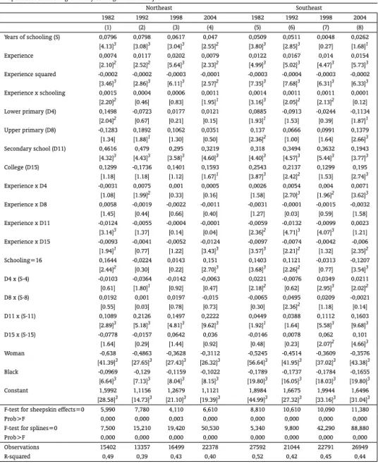
D11 x (S-11) 0,1089 0,2126 0,1497 0,2222 0,0449 0,0388 0,1112 0,1603 [2.89]3 [5.18]3 [4.81]3 [9.62]3 [1.92]1 [1.64] [5.58]3 [9.68]3 D15 x (S-15) -0,0778 -0,0157 0,0642 0,036 -0,0146 0,0078 0,062 0,101 [1.64] [0.29] [1.44] [0.92] [0.48] [0.23] [2.07]2 [4.66]3 Woman -0,638 -0,4863 -0,3628 -0,3112 -0,5245 -0,4514 -0,3609 -0,3576 [41.39]3 [27.65]3 [27.43]3 [26.32]3 [56.64]3 [41.95]3 [37.02]3 [43.38]3 Black -0,0969 -0,129 -0,1159 -0,1022 -0,1789 -0,1737 -0,1784 -0,1655 [6.64]3 [7.13]3 [8.04]3 [8.15]3 [19.80]3 [16.05]3 [18.03]3 [19.80]3 Constant 1,5992 1,1156 1,2679 1,1121 1,8984 1,6675 1,9944 1,6496 [28.58]3 [14.73]3 [21.10]3 [19.39]3 [44.99]3 [27.32]3 [33.16]3 [31.04]3 F-test for sheepskin effects=0 5,990 7,780 4,110 6,610 8,810 10,610 10,090 11,380 Prob>F 0,000 0,000 0,003 0,000 0,000 0,000 0,000 0,000 F-test for splines=0 7,500 15,210 19,420 50,530 5,340 9,800 42,290 88,880 Prob>F 0,000 0,000 0,000 0,000 0,000 0,000 0,000 0,000 Observations 15402 13357 16499 22378 27592 21044 22791 26949 R-squared 0,49 0,39 0,43 0,40 0,52 0,42 0,45 0,44 a_{Note: Robust t-statistics in brackets.}

(17)

Table A-3: Descriptive statistics

1982 1992 1998 2004

Center-west

(957.25) 686,066 1037,66 1004,889 Hourly earnings in the main job 16,51 11,79 17,35 14,37

(25.31) (17.67) (43.59) (32.32)

(4.75) (4.66) (4.52) (4.51)

Age 37,17 37,18 37,81 38,17

(9.16) (9.05) (9.07) (9.20)

Experience 24,39 23,71 24,12 24,17

(10.51) (10.24) (10.39) (10.50)

Number of observations 7499 8835 12030

North

(730,96) (460,36) (694,62) (510,30) Hourly earnings in the main job 14,67 9,89 13,39 10,50

(24,08) (15,42) (22,48) (18,91)

(4,34) (4,47) (4,51) (4,42)

Age 37,28 37,10 37,92 37,71

(9,35) (9,18) (9,05) (9,08)

Experience 24,15 22,72 23,87 23,12

(10,85) (10,63) (10,42) (10,44) Number of observations

South

(857,34) (1201,20) (859,76) (648,93) Hourly earnings in the main job 15,79 12,76 16,53 13,11

(21,81) (27,04) (24,05) (21,08)

(4,40) (4,41) (4,37) (4,34)

Age 37,58 37,76 38,50 39,14

(9,33) (9,09) (9,04) (9,34)

Experience 24,51 23,67 24,68 24,94

(10,65) (10,29) (10,15) (10,50)

(18)

Figure A-1: Educational distribution North South Center-west (a) 1982 0 5 10 15 20 25 30 35

0 1 2 3 4 5 6 7 8 9 10 11 12 13 14 15 16 17

(a) 1992 0 5 10 15 20 25 30 35

0 1 2 3 4 5 6 7 8 910 11 12 13 14 15 16 17

(a) 1998 0 5 10 15 20 25 30 35

0 1 2 3 4 5 6 7 8 910 11 12 13 14 15 16 17

(a) 2004 0 5 10 15 20 25 30 35

0 1 2 3 4 5 6 7 8 9 10 11 12 13 14 15 16 17

(a) 1982 0 5 10 15 20 25 30 35

0 1 2 3 4 5 6 7 8 910 11 12 13 14 15 16 17

(a) 1992 0 5 10 15 20 25 30 35

0 1 2 3 4 5 6 7 8 910 11 12 13 14 15 16 17

(a) 1998 0 5 10 15 20 25 30 35

0 1 2 3 4 5 6 7 8 910 11 12 13 14 15 16 17

(a) 2004 0 5 10 15 20 25 30 35

0 1 2 3 4 5 6 7 8 9 10 11 12 13 14 15 16 17

(a) 1982 0 5 10 15 20 25 30 35

0 1 2 3 4 5 6 7 8 9 10 11 12 13 14 15 16 17

(a) 1992 0 5 10 15 20 25 30 35

0 1 2 3 4 5 6 7 8 9 10 11 12 13 14 15 16 17

(a) 1998 0 5 10 15 20 25 30 35

0 1 2 3 4 5 6 7 8 9 10 11 12 13 14 15 16 17

(a) 2004 0 5 10 15 20 25 30 35

(19)

Table A-4: Earnings equation – North

1982 1992 1998 2004

(1) (2) (3) (4)

Years of schooling (S) 0,0495 -0,065 0,0334 0,0714

[1.81]1 [1.71]1 [0.95] [2.87]3

Experience -0,0013 0,008 0,0143 0,0212

[0.28] [1.19] [2.26]2 [4.95]3

Experience squared -0,0001 -0,0002 -0,0003 -0,0003

[1.12] [2.23]2 _[2.77]3 _[4.80]3

Experience x schooling 0,0007 0,0046 0,0016 -0,0003

[0.80] [3.98]3 _[1.47] _[0.35]

Lower primary (D4) -0,111 0,4838 -0,0501 -0,0405

[1.13] [3.26]3 [0.37] [0.37]

Upper primary (D8) 0,077 0,5483 0,1446 0,0378

[0.67] [4.13]3 _[1.11] _[0.42]

Secondary school (D11) 0,30 0,5511 0,295 0,2851

[2.54]2 _[3.74]3 _[2.22]2 _[3.51]3

College (D15) 0,4938 0,1937 0,4706 0,3075

[3.37]3 [0.85] [2.20]2 [2.58]3

Experience x D4 0,0079 -0,013 0,0033 0,0029

[2.30]2 _[2.58]3 _[0.71] _[0.77]

Experience x D8 -0,0016 -0,0173 -0,0041 0,0045

[0.31] [2.85]3 _[0.74] _[1.22]

Experience x D11 0,0005 -0,0177 -0,0081 0,002

[0.10] [3.09]3 [1.66]1 [0.64]

Experience x D15 -0,0161 -0,018 -0,0198 -0,0135

[2.77]3 _[2.42]2 _[2.80]3 _[3.07]3

Schooling=16 0,1088 -0,0492 0,0624 0,0173

[1.26] [0.46] [0.67] [0.23]

D4 x (S-4) 0,0163 -0,0025 0,0044 -0,0548

[0.75] [0.09] [0.18] [3.06]3

D8 x (S-8) -0,0189 0,0813 0,0376 0,0104

[0.49] [1.97]2 [1.01] [0.43]

D11 x (S-11) 0,0556 0,0814 0,086 0,1933

[1.29] [1.48] [1.73]1 _[7.04]3

D15 x (S-15) -0,0298 -0,054 0,012 0,107

[0.48] [0.66] [0.17] [1.86]1

Woman -0,789 -0,65 -0,5995 -0,5343

[37.00]3 [24.83]3 [26.72]3 [37.13]3

Black -0,1283 -0,1769 -0,1538 -0,1612

[6.03]3 _[6.58]3 _[6.17]3 _[9.66]3

Constant 6,0524 5,3442 5,416 5,1195

[75.86]3 _[44.92]3 _[46.08]3 _[67.22]3

F-test for sheepskin effects=0 6,840 7,740 3,190 5,750

Prob>F 0,000 0,000 0,013 0,000

F-test for splines=0 0,930 4,480 3,630 28,140

Prob>F 0,447 0,001 0,006 0,000

Observations 6300 4201 5127 9928

R-squared 0,45 0,38 0,41 0,41

a_{Note: Robust t-statistics in brackets.}

(20)

Table A-5: Earnings equation – South

1982 1992 1998 2004

(1) (2) (3) (4)

Years of schooling (S) 0,0811 0,002 0,0588 0,0241

[3.53]3 [0.07] [2.18]2 [0.97]

Experience 0,0248 0,0167 0,0193 0,0181

[6.10]3 [3.33]3 [4.12]3 [4.44]3

[7.25]3 _[5.83]3 _[5.83]3 _[5.87]3

Experience x schooling 0,0008 0,0028 0,0007 0,0015

[1.11] [3.43]3 _[0.85] _[2.20]2

Lower primary (D4) 0,185 0,1728 -0,0425 0,0413

[2.48]2 [1.88]1 [0.44] [0.41]

Upper primary (D8) -0,0363 0,2676 0,009 0,2806

[0.40] [2.77]3 _[0.10] _[3.57]3

[2.81]3 _[4.53]3 _[3.97]3 _[3.07]3

College (D15) 0,2663 0,267 0,2777 0,2368

[2.65]3 [2.15]2 [2.29]2 [2.40]2

Experience x D4 -0,0036 -0,003 0,004 -0,0003

[1.39] [0.97] [1.34] [0.10]

Experience x D8 0,0019 -0,0061 0,0031 -0,0091

[0.47] [1.48] [0.85] [2.95]3

Experience x D11 -0,0082 -0,0158 -0,0102 -0,0024

[2.03]2 [3.82]3 [3.00]3 [0.86]

Experience x D15 -0,0026 -0,0132 -0,0086 -0,0087

[0.53] [2.49]2 _[1.95]1 _[2.35]2

Schooling=16 0,0742 0,0952 -0,0504 -0,1205

[1.33] [1.33] [0.83] [2.51]2

D4 x (S-4) 0,0027 -0,0068 -0,0111 -0,014

[0.15] [0.36] [0.64] [0.80]

D8 x (S-8) 0,0104 0,0297 0,0307 0,0137

[0.35] [1.06] [1.37] [0.67]

D11 x (S-11) -0,0137 0,0436 0,0479 0,1127

[0.43] [1.39] [1.81]1 _[5.10]3

D15 x (S-15) 0,0088 0,0682 0,0876 0,1258

[0.21] [1.34] [2.14]2 _[4.02]3

Woman -0,7882 -0,7112 -0,6498 -0,601

[47.68]3 [42.21]3 [46.70]3 [50.74]3

Black -0,1719 -0,1533 -0,1683 -0,1411

[9.19]3 _[6.86]3 _[9.11]3 _[9.38]3

Constant 5,4583 5,3869 5,5152 5,2996

[77.60]3 _[55.94]3 _[59.35]3 _[62.89]3

Prob>F 0,001 0,000 0,000 0,000

Prob>F 0,993 0,001 0,000 0,000

Observations 12355 10700 12245 14832

R-squared 0,52 0,41 0,44 0,42

(21)

Table A-6: Earnings equation Center-west

1982 1992 1998 2004

(1) (2) (3) (4)

Years of schooling (S) 0,0664 0,0383 0,0068 0,0265

[2.81]3 [1.27] [0.25] [1.11]

Experience 0,0104 0,0157 0,005 0,0113

[2.40]2 [2.87]3 [1.00] [2.79]3

[3.34]3 _[3.93]3 _[2.47]2 _[3.99]3

Experience x schooling 0,0017 0,0015 0,0019 0,0009

[2.08]2 _[1.52] _[2.30]2 _[1.24]

Lower primary (D4) 0,1196 -0,1078 0,0007 -0,0691

[1.32] [0.93] [0.01] [0.71]

Upper primary (D8) 0,2629 0,3097 0,3623 0,1938

[2.60]3 _[2.62]3 _[3.45]3 _[2.34]2

[3.73]3 _[3.08]3 _[3.83]3 _[1.87]1

College (D15) 0,2325 0,2805 0,1332 0,1837

[1.96]1 [1.83]1 [0.91] [1.59]

Experience x D4 -0,0004 0,0039 0,0026 0,004

[0.10] [0.97] [0.72] [1.23]

Experience x D8 -0,0082 -0,0099 -0,0108 -0,0045

[1.88]1 _[1.99]2 _[2.52]2 _[1.42]

Experience x D11 -0,0076 -0,0102 -0,0083 0,001

[1.70]1 [2.15]2 [2.04]2 [0.32]

Experience x D15 -0,0091 -0,0047 -0,006 -0,0099

[1.78]1 _[0.77] _[1.18] _[2.34]2

Schooling=16 0,0696 0,0427 0,0304 0,0846

[1.05] [0.50] [0.40] [1.40]

D4 x (S-4) -0,0162 -0,002 0,0004 -0,0084

[0.87] [0.09] [0.02] [0.52]

D8 x (S-8) -0,0349 0,044 0,0268 0,0404

[1.01] [1.32] [0.90] [1.73]1

D11 x (S-11) 0,1454 0,0411 0,1548 0,1608

[3.88]3 _[1.12] _[4.24]3 _[6.07]3

D15 x (S-15) -0,1477 -0,0092 -0,0608 0,0576

[3.14]3 _[0.15] _[1.09] _[1.50]

Woman -0,8387 -0,6843 -0,6668 -0,6177

[46.36]3 [34.69]3 [39.68]3 [44.29]3

Black -0,0873 -0,0941 -0,0949 -0,1356

[5.58]3 _[4.94]3 _[5.59]3 _[9.77]3

Constant 5,5968 5,2684 5,7257 5,4691

[79.48]3 _[55.99]3 _[64.14]3 _[72.36]3

Prob>F 0,000 0,000 0,000 0,003

Prob>F 0,000 0,009 0,000 0,000

Observations 9717 6229 7227 9880

R-squared 0,56 0,46 0,48 0,48

(22)

Figure A-2: Estimated profiles of years of completed schooling and log earnings

Brazil

0 0,5 1 1,5 2 2,5

1 2 3 4 5 6 7 8 9 10 11 12 13 14 15 16 17 1982 2004

Northeast

0 0,5 1 1,5 2 2,5

1 2 3 4 5 6 7 8 9 10 11 12 13 14 15 16 17 1982 2004

Southeast

0 0,5 1 1,5 2 2,5

1 2 3 4 5 6 7 8 9 10 11 12 13 14 15 16 17 1982 2004

North

0 0,5 1 1,5 2 2,5

1 2 3 4 5 6 7 8 9 10 11 12 13 14 15 16 17 1982 2004

South

0 0,5 1 1,5 2 2,5

1 2 3 4 5 6 7 8 9 10 11 12 13 14 15 16 17 1982 2004

Center-West

0 0,5 1 1,5 2 2,5

(23)

Figure A-3: Estimated profiles of years of completed schooling and log earnings – semiparametric re-gressions

earnings – semiparametric regressions.

Brazil

0,0 0,5 1,0 1,5 2,0 2,5

1 2 3 4 5 6 7 8 9 10 11 12 13 14 15 16 17 1982 2004

Northeast

0,0 0,5 1,0 1,5 2,0 2,5

1 2 3 4 5 6 7 8 9 10 11 12 13 14 15 16 17 1982 2004

Southeast

0,0 0,5 1,0 1,5 2,0 2,5

1 2 3 4 5 6 7 8 9 10 11 12 13 14 15 16 17 1982 2004

North

0,0 0,5 1,0 1,5 2,0 2,5

1 2 3 4 5 6 7 8 9 10 11 12 13 14 15 16 17 1982 2004

South

0,0 0,5 1,0 1,5 2,0 2,5

1 2 3 4 5 6 7 8 9 10 11 12 13 14 15 16 17 1982 2004

Center-West

0,0 0,5 1,0 1,5 2,0 2,5