MATLAB GUI for computing Bessel functions
using continued fractions algorithm
(GUI Matlab para o c´alculo de fun¸c˜oes de Bessel usando fra¸c˜oes continuadas)
E. Hern´
andez
1, K. Commeford
2y M.J. P´
erez-Quiles
31
Departamento de Matem´aticas, Universidad de Pinar del R´ıo, Pinar del R´ıo, Cuba 2
Colorado School of Mines, Department of Physics, Golden, CO, USA 3
Instituto Universitario de Matem´atica Pura y Aplicada, Universidad Polit´ecnica de Valencia, Valencia, Spain
Recebido em 11/8/2009; Aceito em 23/1/2011; Publicado em 21/3/2011
Higher order Bessel functions are prevalent in physics and engineering and there exist different methods to evaluate them quickly and efficiently. Two of these methods are Miller’s algorithm and the continued fractions algorithm. Miller’s algorithm uses arbitrary starting values and normalization constants to evaluate Bessel func-tions. The continued fractions algorithm directly computes each value, keeping the error as small as possible. Both methods respect the stability of the Bessel function recurrence relations. Here we outline both methods and explain why the continued fractions algorithm is more efficient. The goal of this paper is both (1) to intro-duce the continued fractions algorithm to physics and engineering students and (2) to present a MATLAB GUI (Graphic User Interface) where this method has been used for computing the Semi-integer Bessel Functions and their zeros.
Keywords: Bessel functions, continued fraction, Matlab GUI.
Fun¸c˜oes de Bessel de ordem mais alta s˜ao recorrentes em f´ısica e nas engenharias, sendo que h´a diferentes m´etodos para calcul´a-las de maneira r´apida e eficiente. Dois destes m´etodos s˜ao o algoritmo de Miller e o al-goritmo de fra¸c˜oes continuadas. O primeiro faz uso de valores iniciais e constantes de normaliza¸c˜ao arbitr´arios, enquanto o segundo o faz calculando cada valor diretamente, minimizando tanto quanto poss´ıvel o erro. Ambos respeitam a estabilidade das rela¸c˜oes de recorrˆencia das fun¸c˜oes de Bessel. Neste trabalho descrevemos ambos os m´etodos e explicamos a raz˜ao pela qual o algoritmo das fra¸c˜oes continuadas ´e mais eficiente. O objetivo do artigo ´e (1) introduzir o algoritmo de fra¸c˜oes continuadas para estudantes de f´ısica e das engenharias e (2) apresentar um GUI (Graphic User Interface) em Matlab no qual este m´etodo foi utilizado para calcular fun¸c˜oes de Bessel semi-inteiras e seus zeros.
Palavras-chave: fun¸c˜oes de Bessel, fra¸c˜oes continuadas, GUI em Matlab.
1. Introduction
Bessel functions arise when using separation of variables to solve some partial differential equations in cylindrical and spherical coordinates [1]. They appear naturally when dealing with Laplace’s and Helmholtz’s equations. The Bessel functions that result as solutions when solv-ing these problems can be applied to various fields, including electricity and magnetism, heat conduction, acoustical vibrations, signal processing, and the radial Schr¨odinger equation [2].
Students are usually introduced to Bessel functions in their partial differential equations class. Attention is focused on the differential equation to obtain Bessel functions, with, usually, very little to the application of such functions. Due to the many applications of Bessel
functions in several scientific fields, a curriculum should be designed to touch on the subject of actually using Bessel functions to solve real-world problems.
While Bessel functions are extremely useful, few al-gorithms exist to calculate them quickly and efficiently. A common method is Miller’s algorithm [3]. Another method is the continued fractions algorithm developed by Ratis and Fern´andez de C´ordoba [4]. These algo-rithms are necessary for various problems in physics. For example, when solving the inhomogeneous Bessel equation, Lommel functions arise. Lommel functions of two variables are superpositions of ordinary Bessel functions, and frequently appear when solving problems in diffraction [1]. When studying scattering problems at high frequencies [5], one must use high order Hankel
3
E-mail: [email protected].
functions, which are linear combinations of Bessel func-tions of the first and second classes. A specific example of using numerical methods to evaluate Hankel func-tions, and therefore Bessel funcfunc-tions, can be found in an article of Havemann and Baran [6]. The continued fractions algorithm can also be use to compute modified Bessel functions and Fresnel integrals [7, 8]. For prob-lems when a numerically reliable and quick algorithm is needed, the continued fractions algorithm (CFA from now on) is a perfect candidate. In all of these exam-ples, we need to know the values of many functions for a given argument at once. While Bessel functions can be easily evaluated using the built-in functions in Mathe-matica or MATLAB, these programs present some lim-itations when several orders and points are needed at the same time.
The goal of this paper is to present the CFA in a pedagogical manner for the use of physics and engi-neering students and for professors to implement in a classroom. We present both algorithms and give the ad-vantages of the CFA, with the help of a MATLAB GUI that we have developed. This GUI can be downloaded
from and it includes
all the algorithms used to compute the Bessel functions and their zeros.
The structure of the paper is as follows: In the second section, we explain the concept of a continued fraction and how it is constructed. The third section presents the two previously mentioned algorithms for evaluating Bessel functions of high order. We give de-tailed descriptions of both Miller’s algorithm and the CFA, and compare the two methods. The fourth sec-tion is devoted to applicasec-tions and examples. Finally, some conclusions are outlined.
2.
Continued fractions
In the mid 17th century, a large number of infinite methods were developed for directly computingπ, in-cluding the method of continued fractions proposed by William Brouncker [9], the president of the Royal So-ciety at the time. However, the theory of continued fractions goes back earlier. In Italy, Pietro Antonio Cataldi had already expressed square roots using this method [10].
Take, for example,√2. If we decompose it into the form√2 = 1 +x, we see that
2 = (1 +x)2↔x2+ 2x= 1→x= 1
2 +x. (1)
If we substitute Eq. (1) into itself, and continue this
substitution indefinitely, we get a continued fraction
x= 1
2 + 1
2 + 1
2 + 1 2 +. . .
. (2)
Following the notation in Wall [11], we define a lin-ear fractional transformation as
z0(x) =b0+x, zn(x) = an bn+x
, n= 1,2,3, . . . ,
(3) where b0 is an integer, and an are positive integers,
which allows us to construct a continued fraction by in-sertingzn(x) as the argument to the previous term and
repeating indefinitely
b0+
a1
b1+
a2
b2+
a3
b3+. . .
. (4)
Consider the sequence given by the successive com-positions of the transformations defined in Eq. (3)
z0z1(x) =z0[z1(x)] =b0+
a1
b1+x
,
z0z1z2(x) =z0[z1[z2(x)]] =b0+
a1
b1+
a
2
b
2+x
, (5)
.. .
z0z1. . . zn(x) =b0+
a1
b1+
a2
b2+· · ·+
an bn+x
, (6)
.. .
From this, we see that
z0z1. . . zn(0) =b0+
a1
b1+
a2
b2+· · ·+
an bn
, (7)
denoting then-th convergent of the continued fraction, withz0(0) =b0 denoting the 0-th convergent.
It is useful to use the equivalent notation for Eq. (5), following the notation of Wallis [12]
z0z1. . . zn(x) =
An−1x+An Bn−1x+Bn
, n= 0,1,2, . . . , (8)
where
A−1= 1, B−1= 0, A0=b0, B0= 1,
An+1=bn+1An+an+1An−1, Bn+1=
which allows us to rewrite then-th convergent in Eq. (7) as
z0z1. . . zn(0) =
An Bn
. (10)
For a continued fraction to have convergence, the limit
lim
n→∞z1z2. . . zn(0) = limn→∞ An Bn
, (11)
should exist and be finite.
An efficient algorithm for calculating continued frac-tions is the Steed algorithm [13]. The method of con-tinued fractions explained in the next section uses the Steed algorithm to calculate a continued fraction.
3.
Bessel function evaluation
Bessel functions are the canonical solutions, ω(z), of Bessel’s differential equation
z2ω′′(z) +zω′(z) + (z2−α2)ω= 0, (12) where α, the order of the Bessel function, is an arbi-trary number that can be either real or complex. Bessel functions of integer order have α = n = 0,1,2, . . .
Semi-integer order Bessel functions, more commonly known as spherical Bessel functions, haveα=n+ 1/2,
n= 0,1, 2, . . .Whenzis a purely imaginary argument, we get modified Bessel functions [14].
Bessel functions are split into two different classes: first class and second class. First class Bessel functions are the solutions to Bessel’s differential equation that are finite at the origin. Second class Bessel functions are the solutions to Bessel’s differential equation that have a singularity at the origin. Usual methods of evaluat-ing Bessel functions use recurrence relations [14]. The class of the Bessel function determines whether we use ascending or descending recurrence relations to obtain the next term in the sequence by either increasing or decreasing n. The direction the recurrence relations take serve to maintain numerical stability [15]. If we were to go the opposite way of the defined relations, the loss of significant figures would skew the results significantly [15].
Second class Bessel functions use an ascending re-currence relation to maintain stability, meaning we can use the first two known values to calculate all higher terms up to some valuen=N. First class Bessel func-tions use a descending recurrence relation to maintain numerical stability. This means that we cannot start from the first two well known values, but must instead find a clever way around this hindrance. A commonly used method to compute Bessel functions is known as Miller’s algorithm [3].
3.1. Miller’s algorithm
Let us consider the first and second class spherical Bessel functions of semi-integer order,jn(z) andyn(z).
The recurrence relations for these two functions are given by
jn−1(z) =2n+ 1
z jn(z)−jn+1(z),
n= 1,2, . . . , (13)
yn+1(z) = 2n+ 1
z yn(z)−yn−1(z),
n= 1,2, . . . (14)
As you can see, Eq. (13) is a descending recurrence relation, and Eq. (14) is an ascending recurrence tion. As we discussed before, using an ascending rela-tion to evaluate jn would lead to absurd results, but
we do not knowjn norjn−1. Miller’s algorithm serves
to “guess”the initial values and re-normalize at a later step.
For a desired value n, we use N > n and as-sume that ˆjN+1 = 0 and ˆjN = 1 and then use
the recurrence relation in Eq. (13) to obtain the se-quence ˆjN−1,ˆjN−2, . . . ,ˆj1,ˆj0. If we have chosen N large enough, the terms of this sequence up to n (i.e.
ˆjn,ˆjn−1, . . . ,ˆj1,ˆj0) will be proportional to the cor-responding term in the sequence jn, jn−1, . . . , j1, j0 of desired values. The proportionality factor p can be obtained by comparing the value of ˆj0 with the known value of j0. The terms of the sequence
pˆj0, pˆj1, . . . , pˆjn−1, pˆjn reproduce the required values j0, j1, . . . , jn−1, jn. If the precision obtained is not
suf-ficient, you can repeat the process with a larger value ofN.
To obtain the second class Bessel functions, we sim-ply use the initial values, y0(z) and y1(z), and apply the ascending recurrence relation until desiredn.
Below is an example of the application of Miller’s algorithm. We have included the same numerical ex-ample as illustrated in the work of Abramowitz and Stegun so that the reader may complete the details in the above work [14].
3.2. Miller’s algorithm example
Suppose we want to evaluate the value of j15(x) for
x = 24.6 using Miller’s algorithm. Let us start, for example, atN= 39 and suppose
ˆ
j40= 0, ˆj39= 1. (15) Using the recurrence
ˆ
jN−1(z) =
2N+ 1
z ˆjN(z)−ˆjN+1(z),
N = 39,38,37, . . . ,1, (16)
we generate the sequence ˆj38,ˆj37, . . . ,ˆj1,ˆj0. If we evaluate
j0(24.6) =
sin(24.6)
we obtain the proportionality factor
p= j0(24.6) ˆ
j0(24.6)
= 0.000000383917642. (18)
The valuepˆj0coincides with the value ofj0(24.6) with 8 correct significant figures [14].
Fortran can be used to evaluate Bessel functions us-ing subroutines of the IMSL library. Numerical analysis for these routines can be found in the work of Ratis and Fern´andez de C´ordoba [4]. These routines are based on Miller’s algorithm.
3.3. Continued fractions algorithm
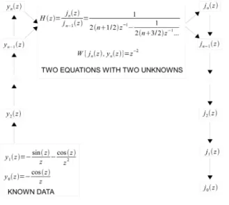
The method of continued fractions introduced in sec-tion 2 can be used to directly evaluate the first class Bessel functions without any normalization. By ap-plying the ascending recurrence relation to the second class Bessel functions, we generate the set{yn(z);n=
0, 1,2, . . . , N}, for a desired value of the ordern=N. We then use the last two values,yN(z) andyN−1(z), a continued fraction, and the Bessel function Wronskian to solve forjN(z) andjN−1(z). We then apply the de-scending recurrence relation to evaluate the first class Bessel functions, {jn(z);n = 0,1,2, . . . , N}. This method achieves the correct values without the need for a normalization factor. Relying on normalization relations to maintain stability hinders the performance
speed of Miller’s algorithm. By disposing of this neces-sity, the CFA runs faster, while still preserving stability by using the appropriate recurrence relations.
In Fig. 1 we present the flowcharts for Miller’s al-gorithm and the CFA to illustrate each method.
We continue to use the usual notation of Abramowitz and Stegun and formally introduce spher-ical Bessel functions of the first and second class [14]
jn(z) =
r
π
2zJn+12(z), (19)
yn(z) = r
π
2zYn+12(z), (20) as solutions to the differential equation,
z2ω′′(z) + 2zω′(z) + [z2−n(n+ 1)]ω(z) = 0, n= 0,±1,±2, . . . (21)
Jn(z) andYn(z) are ordinary Bessel functions of integer order.
With the CFA we can simultaneously calculate the spherical Bessel functions of all orders less than or equal toN,i.e. we generate the set
BE(z)≡ {jn(z), yn(z);n= 0,1, 2,3, . . . , N}. (22)
⌋
We generate all spherical Bessel functions of the sec-ond class, {yn(z), n = 0,1,2, . . . , N}, starting with
the known values of
y0(z) =−cos(z)
z , y1(z) =−
sin(z)
z −
cos(z)
z2 , (23) by using the ascending recurrence relation in Eq. (14) until the fixed valueN.
To calculate the highest order of the first class spher-ical Bessel functions,{jn(z),
n = 0,1,2, . . . , N}, we use the calculated values of
yN(z) and yN−1(z), and the value of the spherical Bessel function Wronskian [14]
W{jN(z), yN(z)} ≡
jN(z)yN−1(z)−jN−1(z)yN(z) =z−2. (24)
We can rewrite Eq. () as
jN−1(z) =
1
z2 Ã
jN(z) jN−1(z)
yN−1(z)−yN(z)
!. (25)
To evaluate the ratiojn/jn−1, we rearrange the re-currence relation forjn(z) given in Eq. (13) to read
jn(z) jn−1(z)=
1
2(n+12)z−1−jn+1(z)
jn(z)
, (26)
allowing us to construct the continued fraction
H(z)≡jjN(z)
N−1(z)
=
1
2(N+12)z−1+ 1
2(N+32)z−1− 1
2(N+52)z−1−. . .
.
(27)
Eq. (27) is easily evaluated using the Steed algo-rithm for a fixed N and z. Using the resulting value, we see that
jN(z) =H(z)jN−1(z). (28) Equations (25) and (28) allow us to generate all spher-ical Bessel functions of the first class, {jn(z), n =
0,1, 2, . . . , N}, by considering the calculated values of
jN(z) andjN−1(z) and using the descending recurrence
relation,
jn−1(z) = 2n+ 1
z jn(z)−jn+1(z). (29)
The CFA maintains the stability of each function by ensuring the use of the proper recurrence relations. Un-like Miller’s algorithm, the CFA directly calculates the
first class Bessel functions, rather than using arbitrary values and normalizing. Miller’s algorithm relies on the normalization process, which requires more values than needed in order to converge to a reasonable proportion-ality factor. This necessity introduces not only another source of error, but also longer calculation times. A detailed numerical analysis can be found in the work of Ratis and Fern´andez de C´ordoba [4].
4.
MATLAB GUI development
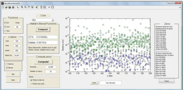
In Fig. 2 we have shown the MATLAB GUI developed for this article. This GUI is divided in four parts. In the left-most section there are several tools to control the functions to plot, number of points, order and pre-cision (Steed tolerance) of the CFA. The user can plot the Bessel function of order n or the complete set of functions from orders 0 ton. It is also possible to layer the graphics using the hold on option, and change the color of the new plots using the first menu of the sec-ond column. The yn(z) functions are plotted using a
continuous line, while thejn(z) functions are shown by a dashed line.
The MATLAB’s Bessel functions section compares the computation times using CFA and MATLAB’s li-braries, and checks the realtive error between CFA and MATLAB codes. It is easy to check that, for n= 50 with 500 points in the range (100,200) of z, CFA code is much faster than MATLAB’s. See Fig. 3 for this ex-ample. In a modern computer, the difference between the computation times of the two methods can be up to two orders of magnitude. In this figure it is possible to see that the relative error distribution in thejn(z)′s
is higher than that ofyn(z)′s.
The last group of the second column and the right-most column are devoted to computing the roots of the Bessel functions. The algorithm that we have im-plemented is a combination of a brute force strategy and a bisection method. First, we compute in the de-sired interval (zmin, zmax) the Bessel functions with (zmax−zmin)∗10 points. Second, using this infor-mation, we compute the zeros in the subintervals where the functions change their sign, using a simple bisection method. There also exists another implementation of the code that computes the desired number of roots starting at zmin. The firsts ten zeros found from each function are displayed in the rightmost part of the fig-ure. Beneath the graph, it is possible to save all the data computed.
4.1. Example
A nice exercise is to compute the zeros of yn(z) and
check how they distribute in space. The same proce-dure can be used to check the zeros of jn(z), but the
Figura 2 - GUI implementation.
Figura 3 - Relative error between CFA and MATLAB. The points with the largest error are close to the roots of the Bessel function involved.
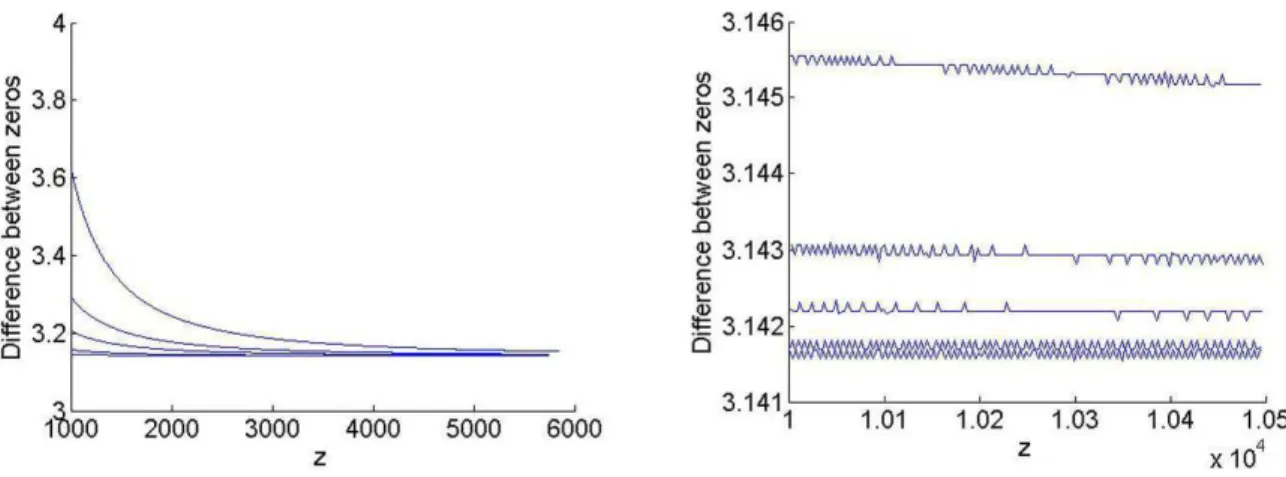
1. Plotyn(z) forn= 50, for example, in the interval
(1000,1200) with 5000 points. It seems clear from the plot that the difference between the zeros is almost constant, see Fig. 4.
2. Compute the zeros of several cases, n = 50,100,200,300,500 for instance. Save the data in file1, file2, file3...
3. Load the data and plot the mean of the difference between the zeros in each case. The following matlab script computes and plots the mean.
orders = [50,100,200,300,500]; meanZeros=zeros(5,1);
figure(2); clf; hold on for i = 1:5
load([’file’,num2str(i)]); meanZeros(i) = mean(diff(y0)); plot(1:length(y0)-1,diff(y0)); end
figure(3); clf; plot(orders,meanZeros,’o’);
It is easy to see in Fig. 5 that the zeros are more dis-persed as we increase the order. However, the student can increase the value ofzminto check that the larger
zis, the closer the difference between zeros is toπ. This is shown in Fig. 6, but one can also prove this statement using asymptotic Bessel function expansions [14].
Figura 4 -y50(z) forz∈(1000,1200).
Figura 5 - Variation of the mean difference between zeros in terms of the order.
Figura 6 - Difference between zeros of theyn(z) whenzis large. Aszincreases, the difference approachesπ.
5.
Conclusions
We have explained how both Miller’s algorithm and the continued fractions algorithm can be used to compute
the method of continued fractions for such computa-tions.
The continued fraction algorithm maintains the sta-bility of each function by ensuring the use of the proper recurrence relations. Unlike Miller’s algorithm, the con-tinued fraction algorithm directly calculates the first class Bessel functions, rather than using arbitrary val-ues and normalizing. Miller’s algorithm relies on the normalization process, which requires more values than needed in order to converge to a reasonable proportion-ality factor. This necessity introduces not only another source of error, but also longer calculation times. A detailed numerical analysis can be found in Ratis and Fern´andez de C´ordoba [4]. A MATLAB implementa-tion of this algorithm, together with a GUI, can be
downloaded from
Acknowledgments
The authors wish to thank the financial support re-ceived from the Universidad Polit´ecnica de Valencia under grant PAID-06-09-2734, from the Ministerio de Ciencia e Innovaci´on through grant ENE2008-00599 and specially from the Generalitat Valenciana under grant reference 3012/2009.
References
[1] B.G. Korenev, Bessel Functions and Their Applica-tions: Analytical Methods and Special Functions, (CRC Press, Boca Raton, FL, 2002)
[2] G.B Matthews and E. Meissel, A Treatise on Bessel Functions and Their Applications to Physics, (Macmil-lan and Co., 1895).
[3] J.C.P. Miller, Bessel Functions, Part II, Functions of Positive Integer Order, Mathematical Tables, Vol. 10, (Cambridge University Press, 1952).
[4] Yu. L. Ratis and P. Fern´andez de C´ordoba, Comput. Phys. Commun.76, 381-388 (1993).
[5] E. Giladi, J. Comput. Appl. Math.198, 52-74 (2007).
[6] S.Havemann and A.J. Baran, J. Quant. Spectrosc. Ra.
89, 87-96 (2004).
[7] J. Segura, P. Fern´andez de C´ordoba, and Yu. L. Ratis, Comput. Phys. Commun.105, 263-272 (1997).
[8] J.L. Bastardo, S. Abraham Ibrahim, P. Fern´andez de C´ordoba, J.F. Urchueguia Sch¨olzel, and Yu.L. Ratis, Appl. Math. Lett.18, 23-28 (2005).
[9] J.L. Coolidge, The Mathematics of Great Amateurs, (Oxford Clarender, 1994).
[10] C.B. Boyer, A history of mathematics (John Wiley Sons, 1968 ).
[11] H.S. Wall, Analytic Theory of Continued Fractions, (Chelsea Publishing Company, Bronx, New York, 1967).
[12] J. Wallis, Opera Mathematica, (Oxonieae e Theatro Shedoniano, 1695, Reprinted by Georg Olms Verlag, Hildeshein, New York, 1972), vol. 1, p. 355.
[13] A.R. Barnett, D.H. Feng, J.W. Steed and L.J.B Gold-farb, Comput. Phys. Commun. 8, 377-395 (1974).
[14] M. Abramowitz and I. Stegun,Handbook of mathemat-ical functions, (Dover Publications, Inc., WA, 1972), pp. 358, 437-453.