AN ALGORITHM FOR DETERMINING THE K-BEST SOLUTIONS OF THE ONE-DIMENSIONAL KNAPSACK PROBLEM
Horacio Hideki Yanasse
Instituto Nacional de Pesquisas Espaciais -INPE/LAC
Nei Yoshihiro Soma
Instituto Tecnológico de Aeronáutica - ITA/IEC Nelson Maculan
Universidade Federal do Rio de Janeiro -UFRJ/COPPE
Abstract
In this work we present an enumerative scheme for determining the K-best solutions (K > 1) of the one dimensional knapsack problem. Ifn is the total number of different items and b is the knapsack’s capac-ity, the computational complexity of the proposed scheme is bounded byO(Knb) with memory require-ments bounded by O(nb). The algorithm was implemented in a workstation and computational tests for varying values of the parameters were performed.
Keywords: Knapsack problem, K-best solutions.
Resumo
Neste trabalho apresenta-se um esquema enumerativo para se determinar as K-melhores (K > 1) soluções para o problema da mochila unidimensional. Se n é o número total de itens diferentes e b é a capacidade da mochila, a complexidade computacional do esquema proposto é limitado por O(Knb). O algoritmo foi implementado em uma estação de trabalho e testes computacionais foram realizados variando-se diferentes parâmetros do problema.
__________________________________________________________________________________ 1. INTRODUCTION
Consider the one-dimensional knapsack problem (KP),
Maximize z =
i n
=
∑
1 cixi
subject to
i n
=
∑
1
aixi ≤ b xi≥ 0 i = 1,2,...,n and integer
Our focus in this work is on the problem of finding the K-best solutions (K > 1) for KP, instead of just a single optimal solution.
The KP is a well known NP-hard problem and is usually considered “well solved”, since there are methods whose running time and space requirements are bounded by pseudo-polynomial functions in the input data, c.f. Toth [1980]; Yanasse and Soma [1987]; Soma, Yanasse, Zinober and Harley [1992]. Additionally, specialized branch-and-bound methods for solving the KP have a good performance in practice, c.f. Martello and Toth [1990].
Contrary to the case K = 1 where there is a vast literature (c.f. Martello and Toth [1990]), the case K > 1 is seldom addressed. We can point out the works by Lawler [1972] and Wolsey [1973], which do not specifically consider the KP but any discrete optimization problem, and more recently, the work of Yanasse and Soma [1990] which addresses the value independent knapsack problem.
Finding the K-best solutions of the Knapsack Problem (KKP) is of interest, for instance, when in addition to the knapsack constraint, there are some others which might be difficult to consider explicitly in a mathematical model, or if considered, would largely increase the size of the model. By finding the best, second best, ..., K-best solution, we are able to sequentially verify these solutions with respect to the additional constraints and stop when a solution that satisfies all of them is found. This situation usually appears in cutting stock problems - in addition to finding good combination of parts to be cut from a larger stock, cutting patterns must obey a series of constraints due to limitations of the cutting machine, material handling problems, order spread, etc.
Related to cutting, there are still other situations where the interest in finding the K-best solutions of a KP may arise. Cutting stock problems can be modeled as a set covering problem where each column represents a possible cutting pattern. In order to use such a formulation, we must gener-ate at least some of the columns of the problem (the possible cutting patterns). The KP might appear as a subproblem for pattern generation, c.f. Gilmore and Gomory [1961, 1963, 1965], where each solution to the KP represents a cutting pattern. Generating a single pattern or several patterns at a time might be of interest, depending on the solution procedure adopted.
Another potential interest for solving the KKP arises in some approaches to integer problems. For instance, Maculan et al [1992] have proposed a column generation method to solve linear programming with bounding variable constraints, extending their results to the solution of integer problems. To solve some integer problems, their method requires a good implementation of an algorithm for the KKP.
the solutions determined. By checking the best K solutions of the scaled knapsack, we are able to verify them and make sure of getting the actual optimal solution for the original problem.
For the K-best KP, branch-and-bound methods do not perform as well as in the 1-best case since branches now cannot be fathomed, lower bounds for the K-best solution being hard to obtain. We are fairly confident that dynamic programming methods and/or other enumeration schemes for solving the K-best KP, are as competitive as any other method in terms of computational effort.
In the following session we propose an enumeration scheme for finding the K-best solutions to the KP. The enumeration scheme proposed allows a better implementation than the general algo-rithms suggested by Lawler [1972] and Wolsey [1973]. In section 3 we present computational tests using the proposed algorithm. Finally, section 4 contains some concluding remarks.
2. The algorithm
Without loss of generality, we assume from now on that the problem data is given in such a way that a1 ≤ a2 ≤....≤ an. For convenience, the KP with equality constraint and right hand side equal to b is denoted by KPb.
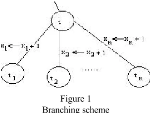
The proposed enumeration scheme is a recursive construction of optimal solutions to KPj for all possible values of the right hand side j, from a1 up to b. It follows closely the one presented in Yanasse and Soma [1987, 1990]. The method proposed can be viewed as an enumeration tree, where at each node we branch adding +1 to each one of the decision variables. So, for instance, at node t, we branch to get nodes t1, t2,…, tn, which are the result of adding 1 to xj, j = 1,..., n to the current solution at t (see Figure 1).
Figure 1 Branching scheme
Following a path from the initial node (node 0) to any node t gives the values to be assigned to the decision variables in order to reach node t. Observe that adding in sequence, +1 to xj, then +1 to xk, ..., then +1 to xs or, by adding in sequence, +1 to xj, then +1 to xs, ..., then +1 to xk leads to the same solution. Hence, to avoid duplications, when branching from a node t, it is sufficient to consider nodes corresponding to adding +1 to decision variables with indices greater than or equal to the index of the incoming branch at node t.
__________________________________________________________________________________ Now, each super node t in the enumeration corresponds to the KPt. And, we know beforehand that in our scheme we are interested in at most (b-a1) super nodes. From each super node t, we update n-j+1 new super nodes (“branching scheme”), where j is the smallest index in super node t for which we know there is a solution for KPt, with xj≥ 1. The super nodes to be updated are the ones determined by adding to t, the coefficient ap, that is, super nodes (t+ap), p = j, j+1,..., n. Of course, only super nodes of interest are updated, that is super nodes (t+ap)≤ b. Observe that the above operation corresponds to adding +1 to the variables with index p, p = j, j+1,...,n. Indices smaller than j need not be considered since the corresponding combinations they produce are considered somewhere else. At each super node are kept the index j known to have at least one solution for KPt with xj≥ 1, together with its corresponding best solution. Observe that the best solution value at a super node (t+ap), corresponding to index p, is obtained by adding to the best optimal solution values at super node t corresponding to indices smaller than or equal to p, the coefficient cp, p = j, j+1,...,n. Starting with super node t = 0, (the root super node, corresponding to KP0) with index set equal to {1,2,...,n} and corresponding objective values {0,0,...,0}, the subsequent super nodes on which to “branch” are always chosen in increasing order of t. Only super nodes having at least one solution are considered. Once a super node t > (b-a1) is reached for branching, we stop. The forward enumeration part has been finished.
We illustrate the forward enumeration scheme by means of a numerical example. Consider the KP:
Maximize z = 4x1+3x2+5x3+7x4+8x5 subject to 3x1+4x2+5x3+6x4+7x5 ≤ 15
xi ≥ 0 i = 1,2,...,5 and integer.
Initially, we start with super node 0, with an attached set of indices {1,2,3,4,5} and correspond-ing values of the objective function {0,0,0,0,0}. Nodes 3,4,...,15 are the other super nodes whose set of indices and corresponding objective function values are to be updated. Observe that super nodes 1 and 2 (all super nodes t < a1) are never updated since they cannot be reached from super node 0 (that is, there is no solution with right hand sides smaller than a1). Since the smaller in-dex in the inin-dex set attached to super node 0 is 1, from super node 0, the following super nodes are to be updated: (0+a1) = 3, (0+a2) = 4, (0+a3) = 5, (0+a4) = 6, (0+a5) = 7. The correspond-ing objective function values are (0+4), (max{0,0}+3), (max{0,0,0}+5), (max{0,0,0,0}+7), (max{0,0,0,0,0}+8), respectively. We represent this information in Table 1.
In Table 1, columns 1 to 5 give indication of the index attached to a super node. The super nodes are indicated in the last column. The numbers filled in the table in any column j are the best ob-jective values corresponding to a feasible solution having at least xj≥ 1. For instance, column 4, node 6, has a value 7, indicating that there is a solution to KP6 with x4≥ 1 and corresponding objective function value equal to 7.
The subsequent super node to branch is super node 3, which is the next super node after 0 that has at least one solution. Since the smaller index in the index set attached to super node 3 is 1 again, from super node 3, the following super nodes are to be updated: (3+a1) = 6, (3+a2) = 7, (3+a3) = 8, (3+a4) = 9, (3+a5) = 10. The corresponding objective function values are (4+4) , (4+3), (4+5), (4+7), (4+8), respectively. This information is shown in Table 2.
Table 1 Initial updating from super node 0
Table 2 Updating from super node 3
Index Index
1 2 3 4 5 SN 1 2 3 4 5 SN
0 0 0 0 0 0 0 0 0 0 0 0
X X X X X 1 X X X X X 1
X X X X X 2 X X X X X 2
4 3 4 X X X X 3
3 4 3 4
5 5 5 5
7 6 8 7 6
8 7 7 8 7
8 9 8
9 11 9
10 12 10
11 11
12 12
13 13
14 14
15 15
__________________________________________________________________________________
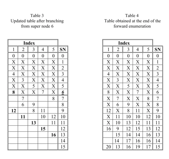
Table 3
Updated table after branching from super node 6
Table 4
Table obtained at the end of the forward enumeration
Index Index
1 2 3 4 5 SN 1 2 3 4 5 SN
0 0 0 0 0 0 0 0 0 0 0 0
X X X X X 1 X X X X X 1
X X X X X 2 X X X X X 2
4 X X X X 3 4 X X X X 3
X 3 X X X 4 X 3 X X X 4
X X 5 X X 5 X X 5 X X 5
8 X X 7 X 6 8 X X 7 X 6
7 8 7 X 7 X X 8 7
6 9 8 X 6 9 X X 8
12 8 11 9 12 X 8 11 X 9
11 10 12 10 X 11 10 10 12 10
13 11 11 X 10 13 12 11 11
15 12 16 9 12 15 13 12
16 13 15 14 14 16 13
14 14 17 16 16 14
15 20 13 16 19 17 15
Recovering the K-best solutions
To recover the K-best solutions a list of the K-best objective function values to the KP is built by traversing the super nodes from b, b-1,...,0, and by choosing the K-best solution values. Unfortu-nately, they are not always the K-best solutions to our KP. There might be alternative solutions with the same objective function value or a little bit smaller which are not explicitly indicated in the final table. It is necessary, therefore, to check the existence of any other alternative solution better than the Kth element listed so far. The only thing that can be stated at this point is that the Kth element in the list is just a lower bound for the K-best optimal solution value of the KP. In our previous numerical example, let us assume K = 15. The initial list containing the best K (=15) objective function values to the KP are: 20, 19, 17, 17, 16, 16, 16, 16, 16, 15, 15, 14, 14, 14 and 13. Hence, a lower bound on the 15th-best objective function value is 13 and a check verifying whether there are other solutions, not explicitly indicated in the final enumeration table, better than the Kth solution, is, then, performed.
The recovering of the K-best solutions is achieved by analyzing the solutions corresponding to the best K values already identified in the list. In the process, we search for alternative solutions having objective values better than the Kth best value identified so far. Our search will start analyzing the best, second best, third best and so on solutions, hoping that by analyzing first the best solutions, there would be an increased chance of finding alternative solutions as good as the ones being considered. Once the analysis of a Jth-best solution with value equal to the Kth best in the list is reached we can stop. The K-best solution values are now at hand and it is necessary only to determine the remaining solutions corresponding to the objective values in the list, which were not considered yet.
Alternative solutions are identified in the process of recovering a solution to a specific objective value, whenever more than one feasible solution is observed in any intermediate super node dur-ing backtrackdur-ing. For instance, in the previous recoverdur-ing process example with super node 15 and objective value 19, a backtrack in super node 9 detected 3 solutions with objective values (12,8,11) identified in the table. All three of them are feasible in the sense that super node 15 can be reached from them and moreover, a numerical value in column 4 indicates that all these values are in columns with indices smaller than or equal to 4. Hence, with all of them, by adding +1 to variable x4, leads to super node 15, column 4. In this example, the objective values correspond-ing to these alternative solutions are different: 19, 15 and 18, respectively. Only one of the solu-tions reaches the value 19, the best value with at least one x4≥ 1.
The full recovery of the 15-best solutions of our numerical example is illustrated now. The proc-ess starts with the 1-best solution value 20. Backtracking, it is seen that the value 20 in super node 15 came by adding +1 to variable x1. Subtracting a1 from 15 yields super node 12, with corresponding objective value of 16 = 20 - c1.
We are again in a similar situation and proceed in the same way, concluding that there is no al-ternative solution for this case. The single solution x1 = 5, x2 = x3 = x4 = x5 = 0, with objective function value 20 has been obtained.
__________________________________________________________________________________ from super node 9, column 4 and objective value 11. We backtrack subtracting a4 from 9. This gives super node 3 with corresponding objective value 4. There is a single solution in node 3 and proceeding with the backtracking up to super node 0 a solution is identified, given by x1 = 1, x4 = 2, x2 = x3 = x5 = 0, with corresponding objective value 18.
Then we return to the smallest super node where an alternative solution was identified, super node 9 in this case. It is necessary now to move to the immediate next column with a smaller index with a solution, that is column 3. A solution of value 8 is found, indicating that a solution exists with corresponding objective function value of 15. Again, this value is compared with the 15th-best value in the list, and since this latter one is greater than the former, it is, therefore, introduced in the list and the previous 15th value is discarded. The lower bound for the 15th-best solution is updated and the process is re-launched from where it has stopped.
Since the last super node considered was the 9, column 3, with objective value 8 a backtracking is performed by subtracting a3 from 9, reaching super node 4 with corresponding objective value of 3. There is just a single solution in super node 4 and proceeding with the backtracking up to super node 0 the solution x2 = 1, x3 = 1, x4 = 1, x1 = x5 = 0, with corresponding objective value 15 is identified.
The smallest super node where an alternative solution was identified, i.e. super node 9 is consid-ered again and the immediate next column, which has yet to be considconsid-ered, with a smaller index possessing a solution is column 1. A solution of value 12 is found, and after a backtracking no more alternative solutions are found, and the single solution x1 = 3, x4 = 1, x2 = x3 = x5 = 0, with corresponding objective function value of 19 is identified.
We move now to the next best value in the list not yet analyzed. At this stage, the list has changed to 20*, 19*, 18*, 17, 17, 16, 16, 16, 16, 16, 15*, 15, 15, 14, 14, where the values indi-cated with an * are the ones which have already been analyzed (the corresponding solutions have already been obtained). The third best value in the list is 18 and it was considered during the analysis of the 2ndbest value. Hence, the 4th-best value, which is 17, is considered next.
Proceeding with the same reasoning, we are in super node 15, column 5, objective value 17, and the backtracking implies in subtracting a5 from 15, reaching super node 8 which has two solu-tions. Starting again the recovering process with the largest index smaller than or equal to 5, a solution of value 9 is found at column 3 in row 8, indicating a solution with corresponding ob-jective function value of 17. We backtrack subtracting a3 from 8 to reach super node 3 with corresponding objective value 4. There is a single solution in node 3 and proceeding with the backtracking up to super node 0 the solution x1 = 1, x3 = 1, x5 = 1, x2 = x4 = 0 is identified, with corresponding objective value 17.
= 3, x3 = 1, x2 = x4 = x5 = 0, with corresponding objective value 17. No more alternative solu-tions are present, so the 6th-best value of the list, which is 16, is examined next.
Proceeding with this analysis, a stage is reached when the 15th-best value is 15 and there are only values 15 in the list to be analyzed. In this case, we are sure that the 15th best value in the list is the optimal value of the 15-best solution of the KP and hence, further searches for alterna-tive solutions are not necessary; what is left is just the recovering of the solution corresponding to each one of the remaining values of the list.
The 15-best solutions to our numerical example are presented in Table 5.
Table 5 15-best solutions to
the example Index
1 2 3 4 5 OV
5 0 0 0 0 20
3 0 0 1 0 19
1 0 0 2 0 18
1 0 1 0 1 17
3 0 1 0 0 17
2 1 1 0 0 16
0 0 0 0 2 16
1 0 1 1 0 16
2 0 0 0 1 16
4 0 0 0 0 16
0 1 1 1 0 15
0 0 3 0 0 15
1 1 0 0 1 15
0 0 0 1 1 15
3 1 0 0 0 15
As can be seen, the memory requirements for the proposed enumeration scheme is O(n(b-a1)). In fact, if K < n, we need to keep only K values for every super node t corresponding to KPt, t = a1,...,b. Hence, memory requirements for the algorithm is O(min{K,n}(b-a1)), and in particular, for K =1, O(b-a1). The computational complexity of the algorithm is bounded by O((K+1)n(b-a1)), since the forward enumeration is bounded by O(n(b-a1)) and to recover the K solutions (any K), we surely require no more than O(K min{K,n}(b-a1)) operations (we, at worse, must back-track this much of the forward enumeration performed, for each one of the solutions). Generally, recovering each solution is quite straightforward taking O((b-a1)/a1) operations, hence, the recov-ery time for the K-best solutions will generally be smaller compared with the forward enumeration time. This was observed with the computational results presented in the next section.
3. Computational experiments
__________________________________________________________________________________ were constructed artificially with all coefficients aj of the knapsack constraint generated ran-domly in the interval [1,5000].
Our proposed enumeration scheme was implemented in C++ on an IBM RISC/6000, Model 580H, with an IBM Power PC 2 processor and 256 Mbytes of RAM memory. All processing times were measured in seconds.
For the first set of tests, we varied the number of the K-best solutions required. K was set to 100, 200,L, 2800, 2900. b was set to 10000 and n to 500. Figure 2 presents the results.
n=500, b=10000 1 3 5 7 9 11 13 15 17 19 21 23 25 27 1 0 0 3 0 0 5 0 0 7 0 0 9 0 0 1 1 0 0 1 3 0 0 1 5 0 0 1 7 0 0 1 9 0 0 2 1 0 0 2 3 0 0 2 5 0 0 2 7 0 0 2 9 0 0 K sec
Forward Backward TOTAL
Figure 2
Computational times with varying K
In the second set of problems we varied the number of variables n. n varied from 100 to 1050 in steps of 50. K and b were fixed respectively to 1000 and 10000. The results are shown in Figure 3. K=1000, b=10000 0 2 4 6 8 10 12 14 16 1 0 0 1 5 0 2 0 0 2 5 0 3 0 0 3 5 0 4 0 0 4 5 0 5 0 0 5 5 0 6 0 0 6 5 0 7 0 0 7 5 0 8 0 0 8 5 0 9 0 0 9 5 0 1 0 0 0 1 0 5 0 n sec
Forward Backward TOTAL
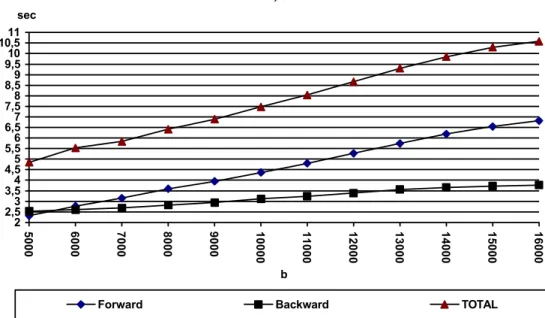
In the last set of tests we varied the value of b from 5000 to 16000, in steps of 1000. The number of variables and K were fixed in 500 and 1000, respectively. The results are presented in Figure 4. K=1000, n=500 2 2,53 3,5 4 4,5 5 5,5 6 6,5 7 7,5 8 8,5 9 9,5 10 10,5 11 5 0 0 0 6 0 0 0 7 0 0 0 8 0 0 0 9 0 0 0 1 0 0 0 0 1 1 0 0 0 1 2 0 0 0 1 3 0 0 0 1 4 0 0 0 1 5 0 0 0 1 6 0 0 0 b sec
Forward Backward TOTAL
Figure 4 Effect of varying b
The forward enumeration becomes responsible for most of the processing time, as n increases. Retrieving the solutions demands an amount of time which depends on K and n, but we observed that it is quite insensitive with respect to variations in the value of b (perhaps because of the small variations of this parameter for the tests performed). Its contribution to the overall com-puter processing time sharply decreases (percentagewise) as the size of the problem increases. For K < n, the time complexity of the recovery phase should vary as K2b and for K > n as Knb. The backward curve in Figure 2 suggests a quadratic behaviour with K, even for K larger than n. A possible explanation for this behaviour is due to the fact that all the tests were run using the same implemented version of the algorithm where the number of columns was maintained fixed. Recall that in case of K < n, only K columns are needed to be carried on in the forward enu-meration. Another explanation is the computational time spent to sort the solutions. Recovered solutions are sorted as they are obtained, however, no special care was taken to use an efficient sorting routine in the implemented version of the algorithm. Therefore, the curves in Figure 2 are overestimating the actual ones that would have been obtained with an improved implementation.
4. Concluding remarks
__________________________________________________________________________________ The proposed enumeration scheme can be easily extended to solve knapsack problems with bounded variables, in particular the 0-1 case. Notice that the equality constrained KP can also be easily solved. In fact it was solved as a by-product of our proposed enumeration scheme.
Improved computational time performance might be obtained if additional information are kept. For instance, we can keep in another array, the index and the best value for each super node. Hence, these optimal solutions for each KPt, will be ready for consulting when needed, other-wise, every time we need such information at each super node, it is necessary to make a search amongn elements.
It is of course possible to have an implementation of the algorithm with a reduced memory re-quirement. The authors can propose an implementation using O(b-a1) of memory space but the computational effort to recover the solutions will be much increased.
We would like to observe that the proposed enumeration scheme presented is just the KP solved as a longest path problem, where we are interested in finding the longest path from node 0 to node b. The "distance" from a node j to a node j+ak in the "knapsack graph" is given by ck, for each one of the nodes j = 0, 1, 2,..., b, and for every k = 1,2,..., n (see Figure 5).
0 1 2 j j+a b
k c
k
c 1
c n
0 0 0
0 0
.. .
. .
.
. ..
Figure 5
KP as a longest path problem
With the implementation proposed here many arcs of the graph are not considered, thus avoiding duplicated analysis of equivalent solutions. Additional information of intermediate paths is kept so that information on alternative solutions and not only the best solution are retrieved with in-creased efficiency. It is important to note that other known algorithms for solving the KKP, based on the approach suggested previously, e.g. Katoh, Ibaraki and Mine [1982], Perko [1986], Sckiscim and Golden [1989] and, more recently, Eppstein [1994], are designed for the 0-1 case. No direct comparison among those methods with the one suggested here can be made, since the corresponding number of varivables (n) increases for the 0-1 case, which, in turn, affects the quantity of arcs in the "knapsack graph".
Note that the computational complexity of finding the K-longest loopless paths from node 0 to node b, in a general network with (b+1) nodes using the proposed enumeration scheme is O((K+1)b2). Exactly the same reasoning can be applied to find the K-shortest loopless paths in a network, hence, with the same computational complexity. Observe that in terms of computational complexity this scheme to solve the K-shortest loopless paths in a network is better than the one suggested by Lawler [1972] which requires O(Kb3).
Pesquisa do Estado de São Paulo. The authors also thanks for the comments of the anonymous referees that improved the presentation of the paper.
References
(1) Eppstein, D. (1994) Finding the k Shortest Paths,Proc. 25th IEEE Annual Symposium on Foundation of Computer Science, 154-165.
(2) Gilmore, P.; Gomory, R. (1961) A linear programming approach to the cutting stock prob-lem.Operations Research,9, 849-859.
(3) Gilmore, P.; Gomory, R. (1963) A linear programming approach to the cutting stock problem - part II. Operations Research,11, 863-888.
(4) Gilmore, P.; Gomory, R. (1965) Multistage cutting stock problems of two and more dimen-sions.Operations Research,14, 1045-1074.
(5) Katoh, N.; Ibaraki, T.; Mine, H. (1982) An efficient algorithm for the shortest simple paths, Networks,12, 411-448.
(6) Lawler, E.L. (1972) A procedure for computing the k-best solutions to discrete optimization problems and its application to the shortest path problem. Management Science,18 (7), 401-405.
(7) Maculan, N.; Michelon, P.; Plateau, G. (1992) Column-generation in linear programming with bounding variable constraints and its application in integer programming. Pesquisa Op-eracional,12 (2), 45-57.
(8) Perko A. (1986) Implementations of algorithms for k shortest loopless paths, Networks, 16, 149-160.
(9) Martello, S.; Toth, P. (1990) Knapsack problems - Algorithms and Computer Implementa-tions. John Wiley & Sons, Chichester.
(10) Sckiscim C.C. and Golden, B.L. (1989) Solving k-shortest and constrained shortest path problems efficiently, Annals of Operations Research,20, 249-282.
(11) Soma, N.Y.; Yanasse, H.H.; Zinober, A.S.I.; Harley, P. J. (1992) A pseudopolylogarithmic algorithm for the subset sum problem. CO92 - Combinatorial Optimization Conference, Uni-versity of Oxford, Oxford, England.
__________________________________________________________________________________
(13) Wolsey, L.A. (1973) Generalized dynamic programming methods in integer programming. Mathematical Programming,4, 222-232.
(14) Yanasse, H.H.; Soma, N.Y. (1987) A new enumeration scheme for the knapsack problem. Discrete Applied Mathematics,18, 235-245.
(15) Yanasse, H.H.; Soma, N.Y. (1990) Finding the k-best solutions to a value independent knapsack problem. IFORS XII, Athens, Greece.
Appendix – The K-best algorithm Given
positive integers b,n, K,ai,i = 1, 2, ..., n, such that
n≤Kanda1≤a2≤....≤an,
non-negative real numbers ci,i = 1, 2, ..., n. If for some i, ai=ai+1thenci≥ci+1. Notation
• Variables in bold indicate vectors;
• 0is a vector with all components equal to 0. • 1is a vector with all components equal to 1. • // line with comments
The algorithm
Main Program
Begin-Main
// Begin-Initialization Generate matrix MbXn
M(r,s)← -1, r= 1,...,b and s= 1,...,n // End-Initialization
// Begin-Forward Enumeration // Begin initial ramification
Forj = 1 to n do M(aj,j)←cj; // End-initial ramification
// Begin-ramification of supernodes Fort = a1 to (b- a1) do
Begin-For m←n+1;
m← min {i : M(t,i)≥ 0, i = 1, …n}; If (m≠n+1)Then
Begin If
z←M(t,m); Fori = mtondo Begin-For
If (M(t,i) > z)Thenz←M(t,i); M(t+ai,i)←z+ci;
End-If End-For
End-If End-For
// End-ramification of supernodes // End-Forward Enumeration // Begin-Backward Recovering
ExecuteBuild-initial-best-K-list (L,P,K)
// P is equal to K if there are at least K best values available; L(i) is the ith best solution in // the list and is characterized by 5 attributes: L(i).X the vector solution, L(i).V the
// objective function value, L(i).J and L(i).T which are, respectively, the original column // and line in matrixMbXn where the solution was identified, and L(i).C, an 0-1 control
// variable that indicates whether the vector solution L(i).X has already been // recovered or not.
ExecuteRecover-solution(L,P,K) // End-Backward Recovering End-Main
ProcedureBuild-initial-best-K-list (L,P,K) Begin // Build-initial-best-K-list
// List of K elements are ordered at a time. Lists are combined when necessary. Many other // alternative ways to find the initial K-best elements exist (e.g. Binary Search Tree
// with post-order) Counter← 0; i←b+1; Fim←False; Moreleft←False; While (i > a1)do Begin-While
i←i-1; j←n+1; While (j > 1) do Begin-While
j←j-1;
If (M(i,j)≥ 0) Then Begin-If
Counter←Counter + 1; L(Counter).V←M(i,j); L(Counter).J←j; L(Counter).T←i; If (Counter = K)Then Begin-If
i1←i; j1←j;
Moreleft←True; i← 0;
__________________________________________________________________________________ End-If
End-While End-While P←Counter;
Sort in non-increasing order, L(i)i = 1, ..., P, using attribute L(i).V If ((P = K).AND.(( i1 > a1).OR.( j1 > 1)) ThenFim←True; While (Fim)do
Begin-While Counter← 0; i←i1+1; Fim←False; While (i > a1)do Begin-While
i←i-1; j←n+1;
If (Moreleft)Then Begin-If
j←j1;
Moreleft←False; End-If
While (j > 1) do Begin-While
j←j-1;
If (M(i,j) > L(K).V ) Then Begin-If
Counter←Counter + 1; L1(Counter).V←M(i,j); L1(Counter).J←j; L1(Counter).T←I; If (Counter = K)Then Begin-If
i1←i; j1←j;
Moreleft←True; i← 0;
j← 0; End-If End-If End-While End-While P1←Counter;
Sort in non-increasing order, L1(i)i = 1, ..., P1, using attribute L1(i).V
If (L1(1).V > L(K).V)Then using lists L and L1, build a sorted list (non-increasing or-der) of the K objects having the largest V attribute. Assign this list to L(i),i = 1, ..., K; If (( i1 > a1).OR.( j1 > 1)) ThenFim←True;
End-While Fori = 1 toPdo Begin-For
End // Build-initial-best-K-list
ProcedureRecover-solution(L,P,K) Begin // Recover-solution
i← 0;
While (i≤P)do Begin-While
i←i+1;
If (L(i).C= 0)Then Begin-If
AUXL←L(i);
CallBacktracking (L, AUXL,i,P,K); L(i)←AUXL;
End-If End-While
End // Recover-solution
ProcedureBacktracking (L,AUXL,i,P,K) Begin // Backtracking
t←AUXL.T; j←AUXL.J; z←AUXL.V; zcum← 0; While (t > 0) do Begin-While
t←t–aj; z←z – cj;
zcum←zcum+cj;
AUXL.X(j)←AUXL.X(j)+1; j← {s : M(t,s) = z,1≤ s ≤ j}; j1←AUXL.J;
If (t > 0) Then CallSearch-alternative-solution (t,j,zcum,j1,i,L,P,K); End-While
AUXL.C ← 1; End // Backtracking
ProcedureSearch-alternative-solution (t,j,zcum,j1,i,L,P,K) Begin // Search-alternative-solution
Fors = 1 toj1do Begin-For
If (s≠j)Then Begin-If
If (M(t,s)≥ 0) Then Begin-If
If ((M(t,s)+zcum)≥L(P).V)Then Begin-If
__________________________________________________________________________________ f←P;
While (f > g)do Begin-While L(f)←L(f-1); f←f-1; End-While
L(g).V←M(t,s) + zcum; L(g).J←L(i).J;
L(g).T←L(i).T; AUXL1.V←M(t,s); AUXL1.J←s; AUXL1.T←t; AUXL1.X←0;
CallBacktracking (L,AUXL1,g,P,K); L(g).C← 1;
L(g).X←L(i).X + AUXL1.X; If (M(t,s)≥L(P).V)Then Begin-If
Determine position k : k > g to insert this alternative solution in ordered list L; If (P < K)ThenP←P+1;
f←P;
While (f > k)do Begin-While
L(f)←L(f-1); f←f-1; End-While L(k)←AUXL1; End-If
End-If End-If End-If End-For