Sba Controle & Automação vol.22 número4

(1)

VIRTUAL INTERPOLATION OF DISCRETE MULTI-OBJECTIVE

PROGRAMMING SOLUTIONS WITH PROBABILISTIC OPERATION

Ricardo C. Silva

∗

[email protected]

Edilson F. Arruda

†

[email protected]

Fabrício O. Ourique

‡

[email protected]

∗_{Institute of Science and Technology, Federal University of São Paulo}

Rua Talim, 330, São José dos Campos, SP, 12231-280, Brazil. †_{Department of Production Enginnering}

Alberto Luiz Coimbra Institute for Graduate Studies and Research in Engineering Federal University of Rio de Janeiro

P.O. Box 68507, Rio de Janeiro, RJ, 21941-972, Brazil ‡_{Computer Engineering, Federal University of Pampa, Campus Bagé}

Travessa 45, 1650, Bagé, RS, 96413-170, Brazil

RESUMO

Interpolação virtual de soluções de programação multi-objetivo discreta com operação probabilística

Apresenta-se, neste trabalho, um novo método para se tratar a operação em horizonte infinito de uma classe de problemas de programação multi-objetivo. A abordagem proposta con-sidera uma operação estocástica e avalia o custo/lucro médio em horizonte infinito. Para ilustrar a abordagem proposta, um método de duas fases é proposto para resolver um número pré-determinado de K problemas multi-objetivos, de modo a se identificar um conjunto com K pontos pertencentes à re-gião Pareto-ótima. A segunda fase consiste em se buscar um conjunto não-dominado de distribuições de probabilidade no domínio dos K pontos de operação selecionados na primeira fase, que define a probabilidade de se escolher cada um dos pontos de operação em todo instante de decisão. Cada dis-tribuição de probabilidade gera um vetor de funções obje-tivo no longo prazo e determina-se o conjunto Pareto-ótimo com respeito às médias dos objetivos. A abordagem proposta

Artigo submetido em 21/05/2010 (Id.: 01152) Revisado em 26/09/2010, 07/02/2011

Aceito sob recomendação do Editor Associado Prof. Ivan Nunes Da Silva

pode gerar pontos de operação virtuais, com médias de fun-ção objetivo que não necessariamente correspondem a um ponto factível de operação. Alguns experimentos numéricos são desenvolvidos para ilustrar a abordagem proposta.

PALAVRAS-CHAVE: Otimização de Pareto, Operação

dinâ-mica, Otimização discreta

ABSTRACT

(2)

to the average objectives. The proposed approach can gener-atevirtualoperating points with average objectives that need not have a feasible solution with an equal vector of objec-tives. A few numerical examples are presented to illustrate the proposed method.

KEYWORDS: Pareto-optimality, Dynamic operation,

Dis-crete optimization

1 INTRODUCTION

Humans have to choose among a finite number of alternatives to make decisions according to some criterion or objective. However, many real-world problems do not involve a single objective. Rather, they have multiple, possibly conflicting objectives to be optimized simultaneously. The wide range of problems in this category motivated the development of the field of Multiple Criteria Decision Making (MCDM), also known as Multi-Objective Programming (MOP). This field dates back to the early works by PARETO (1897a) and PARETO (1897b) that introduced the concept of corporative equilibrium. A survey about the history and social motiva-tions for the development of this equilibrium concept is pre-sented by STADLER (1979); it covers the interval between 1776 and 1960. CHANKONG and HAIMES (1983) present a formulation of the MOP problem in the space of the objec-tives, as well as some definitions of Pareto-optimality con-cepts that are used in most of the existing MOP methods.

As the term suggests, MCDM is a branch of Operational Re-search (OR) primarily concerned with decision problems in-volving multiple objectives, e.g. (ZIONTS, 1992). The fun-damental guidelines regarding the decision making in multi-objective problems can be found in the work by KEENEY and RAIFFA (1976). An effort is conducted by REID and CITRON (1971) to establish some basic properties of the noninferior surface in general multi-objective problems. In another line of research, conditions for the existence of a single optimal solution to multi-objective problems were investigated in (ATHANS and GEERING, 1973; SALUK-VADZE, 1974). A study on sensitivity analysis tools, de-signed to investigate the influence in the output of any given change in the input, was presented by INSUA (1990).

One way to tackle MOP problems involves defining a map-ping from the set of feasible solutions to function space. Such a mapping is often called utility function and allows a complete ordering of the set of feasible solutions. There-fore, the knowledge of the utility function makes it possible to reformulate a MOP as an ordinary mono-objective opti-mization problem with the utility function acting as the ob-jective. However, in many situations it is not possible to identify or assess a utility function. In those cases, a par-tial ordering of the feasible solutions in terms of the values

of the individual objective functions can be used. Under such an ordering, one can identify particular solutions that cannot be thoroughly improved, i.e. solutions such that no other solution exists that improves all objective functions simulta-neously. Any solution of this type is callednondominated, and multi-objective programming methods are developed to identify the set of nondominated solutions, also known as the Pareto-optimal setorPareto front(or subsets of it). After a set of nondominated solutions is identified, it is handed in to the decision maker and she is assigned the task of choosing a particular solution from this set.

(3)

de-termine a set of waste collection points for different sorts of waste in a urban region.

Even though the MOP formulation of any given system is static, it can be related to the dynamic operation of the sys-tem. Think, for instance, of a multi-objective allocation prob-lem in which clients are allocated to existing facilities first thing in the morning on every business day. If the decision maker criterion does not change during a given stretch of time, the same allocation is selected every single day during that time interval. In such a problem, a vector comprised of the averages of all objective functions during the selected in-terval (which in this case coincides with the vector of objec-tive functions at the selected operating point) can be used as an alternative objective function. It is worth pointing out that, although the MOP literature is rich and vast, there are not, to the best of our knowledge, works dealing with the dynamic or probabilistic operation of systems and multi-objective cri-terion. It is the probabilistic selection of operating points for the dynamic operation of MOP systems that we address in this work.

The contribution of this paper is to introduce a novel framework for dynamic multiple criteria decision making (MCDM). The paper proposes a probabilistic selection of the operating point for systems with static or slowly changing decision making criteria. The proposed framework can be viewed as a generalization of the classicalstaticMOP frame-work. Under the former, one is concerned with selecting an operating point for the system under multiple (possibly con-flicting) optimization criteria. The latter, on the other hand, deals with the dynamic operation of the system. This in-volves selecting different operating points and establishing rules that govern the switch between any two of the selected operating points.

The paper is organized as follows. Section 2 presents the mathematical formulation and the basic concepts of multi-objective programming. Section 3 describes and motivates the proposed probabilistic approach to multi-objective pro-gramming. Section 4 features a procedure for selecting of op-erating points and establishing transition probabilities among these points. Section 5 presents a numerical simulation for a facility location problem and an analysis of the obtained out-comes. Finally, concluding remarks can be found in Section 6.

2 TRADITIONAL MATHEMATICAL

FOR-MULATION

A classical multi-objective problem can be formulated as fol-lows:

Minimize F(x)

Subject to x∈Ω (1)

whereF= [f1,f2, . . . ,fm]T,(m≥2)is a vector of objectives andΩis the set of feasible solutions.

Often the objectives are conflicting and there exists no feasi-ble solution that minimizes all objectives simultaneously. To tackle this problem, one uses the concept ofnon-dominated solutions. This concept was introduced in Vilfredo Pareto’s classical works (PARETO, 1897a; PARETO, 1897b). A so-lutionx∗_∈Ω_{is said to be}_{non-dominated}_(or_{Pareto-optimal}_,

orefficient) if there exists no alternative solution inΩthat is best or equal in all objectives simultaneously and that strictly improves at least one objective.

For any pairx,y∈Ω, x6=y, define the following partial or-dering in terms of the objectives in Problem (1):

F(x)≤(≥)F(y)if fi(x)≤(≥)fi(y),∀i∈ {1, . . . ,m}

F(x)<(>)F(y)ifF(x)≤(≥)F(y)andF(x)6=F(y) (2)

WhenF(x)<F(y)we say thatx dominates y. On the other hand, ifF(x)>F(y), we say thatx is dominatedbyy. Note that, when a feasible solutiondominates another one, it is certainly a better solution to (1) than its counterpart; when it is dominated by the counterpart, it is certainly a worse solu-tion to (1). Based on the relasolu-tions in (2) one can construct the following sets for any pointx0∈Ω

Ω<(x0) , {x:F(x)<F(x0)}

Ω≥(x0) , {x:F(x)≥F(x0)}

Ω∼(x0) , {x:F(x)F(x0) e F(x)F(x0)},

(3)

Observe that:

1. Ω=Ω<(x0) S_Ω

≥(x0)SΩ∼(x0).

2. Ω<(x0) and Ω≥(x0) denote, respectively, the set of

points inΩthat dominate and are dominated byx0.

3. Ω∼(x0)lists every point inΩwhich cannot be compared

tox0according to the partial ordering employed. 4. For any global (efficient) solution tox∗_∈_Ω_{to (1),}_Ω_∩

Ω<(x∗) =/0.

A local (locally efficient) solution to (1) can also be defined in terms of the sets introduced above. We say thatx∗ _{is a}

local solution to the problem in question whenever

B₍_x∗_,_ε₎_∩_Ω

<(x∗) =/0,

for some scalarε>0, whereB₍_x∗_,ε_{) =}_{_x_∈Ω _: _k_x₋_x∗_k_<

ε};k · kdenotes the Euclidean norm.

(4)

1983; MARLER and ARORA, 2004; CHINCHULUUN and PARDALOS, 2007). These methods are classified according to the instant the decision maker applies their criteria. Three methods are proposed: (i)a-Priori method, where the de-cision maker assigns preferences to the objective functions a priori, thus obtaining a single mono-objective criterion; (ii)a-Posteriori method, where the decision maker strives to create a set of (locally) efficient solutions to choose from a posteriori; and (iii)interactive methods, where the decision maker informs their preferences during the search for an ef-ficient solution. The first category is used when the deci-sion maker has preferences concerning the objectives. In this category, one can highlight thelexicographic method, which requires a list of objectives in decreasing order of preference and thebounded objective function method, that selects a sin-gle most preferred objective function and transforms the re-maining objectives into constraints with fixed bounds chosen by decision maker. The second category aims at generat-ing a set of non-dominated solutions to be chosen from at a later stage by the decision maker. This category features theweighted method, which obtains each point in the non-dominated set as a solution to a transformed single objective problem, where the objective is a convex combination of the original objective functions, and theε-constrained method, which is similar to the bounded objective function, but where the bounds are not flexible. The last category obtains the de-cision maker’s preferences during the run of the algorithm, with a view of generating a desirable operating point. Un-der this framework, one can highlight the STEP method, which is exact and the evolutionary algorithm GENOCOP, e.g, (SAKAWA and YAUCHI, 1998). It is worth pointing out that evolutionary algorithms are used to seek solutions in all three categories. However, they are typically classified as a-Posteriori methods.

The traditional formulation described above will help us in-troduce in the next section the motivation of this work. We shall work with a generalized dynamic approach that re-sults in a multi-objective linear formulation, regardless of the structure of the objective functions in (1). The classical for-mulation serves as a reference for comparison, and can also be used to generate the operation points to be used in the dynamic operation of the system being optimized.

3 THE PROPOSED PROBABILISTIC

FOR-MULATION

For systems with a dynamic, repetitive operation, one can di-vide the time horizon in discrete periods and redefine Prob-lem (1) in terms of the long term average cost of the objective functions. LetXk, k≥0, denote the operating point in period

kand define the following problem in

Minimize lim K→∞

1 K

K

∑

k=0 F(Xk) Subject to Xk∈Ω

(4)

Note that problem (1) can be viewed as a specialized version of the proposed problem (Eq. (4)), withXk=x, ∀k≥0.

In the proposed approach, we assume that at each discrete periodk≥0, the system operates in a given pointx∈Ωwith probability µ(x)∈[0,1]. In such a setting, Xk, k≥0 be-comes an homogeneous Markov chain (BRÉMAUD, 1999) with transition matrix P=pxy, with pxy=µ(y),∀x,y∈Ω and problem (4) becomes

Minimize lim K→∞

1 K

K

∑

k=0

F(Xk) =

∑

y∈Ω

µ(y)F(y), (5)

where the last equality is a consequence of the strong law of large numbers (BRÉMAUD, 1999). The last equality also follows by noting thatµ:Ω→[0,1]is a stationary distribu-tion for processXk,k≥0, e.g. (BRÉMAUD, 1999, Theorem 3.4.1).

Note that, although Problem (5) can be viewed as a gener-alization of Problem (1), once the operating points are set, it becomes a linear programming problem, regardless of the definitions of the objective functions fi, i∈ {1, . . . ,m}. In contrast, the latter (static) problem is only linear when all objective functions are linear. Hence, the solution to the gen-eralized Problem (5) can be, in fact, easier to find than the solution to Problem (1).

This paper addresses systems with static or slowly changing decision making criteria. Such systems yield long time inter-vals of operation under the same criterion. In that scenario, we can assume that the length of the operating window under a given decision criterion, denoted here asK, tends to infin-ity. At each window, one is faced with an static problem of selecting a probability distributionµin the setΠof feasible distributions fromΩto the interval[0,1]and the objective is

to find the set of non-dominated distributions with respect to the vector of average objectives

F(µ) =

∑

x∈Ω

µ(x)F(x), µ∈Π, (6)

whereF= [f1 f2. . . fn]T is the vector of objective functions; the superscriptT denotes the transpose of a vector.

(5)

3.1 Selection of a Finite Set of Operating

Points

Within the general proposed framework, one applies Eq. (6) to find a probability distribution that shall determine the probability of selecting eachx∈Ωas the operating point at a given period. An obvious simplification is to select a finite set of operating points inOp⊂Ωand make the system op-erate exclusively within this set. This is equivalent to setting µ(x) =0, ∀x∈/Op. It opens the possibility of selecting op-erating points within thestaticPareto-optimal set. It is this approach that we will further exploit in the next section.

Note that the proposed approach is founded in the repetitive operation of a given system. The operation of the system can be divided in discrete periods and, at the onset of each period, the decision maker chooses the operation point to be utilized in that period. Any operating pointx∈Opcan be selected with probabilityµ(x)≥0. At each new period this process is repeated, and the long term average operating cost of the system can be assessed with the help of Eq. (6), where µ(x) =0, ifx∈/Op.

3.2 Motivations and Discussions

To illustrate the proposed approach, consider the follow-ing hypothetic two-objective optimization problem with only two feasible solutions, as depicted in Fig. 1.

f1(x)

f2(x)

F(a)

F(b)

Figure 1: Operating Points in a Multi-Objective Problem

Using the traditional static MOP approach, the decision maker would choose either a or b as the operating point for the MOP problem and the long term average cost would be either F(a) or F(b). It is worth noting that F(a) = [f1(a) f2(a)]T andF(b) = [f1(b) f2(b)]T are two-dimensional vectors comprising both objective functions.

By setting a probability distributionµ:{a,b} →[0,1] and applying formulation (5), one can emulate a relaxed version

of the problem with an expanded operating region. While thestaticformulation must choose to operate either at point a, paying a long term average costF(a)or at pointb, paying F(b), the dynamic formulation allows one to select any con-vex combination ofF(a)andF(b)as the long time operating cost of the system. It can be argued that each probability dis-tribution generates avirtualoperating pointc, with average long term cost

F(c) =µ(a)F(a) +µ(b)F(b)

It is worth noting that a real operating point d ∈Ω, with F(d) =F(c)need not exist. Hence, the proposed approach can, in fact, expand the operating region by generating vir-tualoperating points whose objective function cannot be em-ulated by any point within the feasible setΩ.

Observe in Fig. 2 that virtual operating points with aver-age operating costs in the line connectingF(a)andF(b)can be generated by setting appropriate probability distributions. Thevirtualoperating pointcis only an example correspond-ing to an specific probability distribution ˆµ. In Fig. 2, the values fi(c) =µˆ(a)fi(a) +µˆ(b)fi(b), i=1,2. Observe also that the virtual operating region expands the operating region from the discrete setΩ={a,b}to a continuous set, whose objective function vectors are depicted in Fig. 2.

f1(x)

f2(x)

f1(c)

f2(c)

F(a)

F(b)

F(c)

Virtual operating region

Figure 2: Feasible Solutions in a Multi-Objective Problem

(6)

Observe that the generation of avirtual probabilistic oper-ating point that does not have an equivalent solution inΩis possible and it does not involve operation outside ofΩ.

Another possible application of the proposed formulation is to facilitate the management of the system operation in the long run. With system operation being constrained to a small number of vertex points - such as a few points selected from the Pareto-optimal set, also known as thePareto front- the setup (transition) costs and times tend to decrease as time elapses, creating a very specialized environment. Moreover, to change virtual operating points one only needs to alter the probability distributionsµ:Ω→[0,1], which does not dis-turb the operation of the system by adding unexperienced op-erating points. This can be advantageous, since the Pareto-optimal region often contains an infinite number of points and any change in the operating point within the original MOP framework will very likely involve a transition to an operating point never experienced before. The lack of expe-rience with such a transition may render the operation trou-blesome and expensive in terms of setup time and cost.

The proposed probabilistic approach can also be employed as a method to manage customer dissatisfaction. It may be used to add flexibility to the operation of the system in the long run and help managing marginal costs which may be difficult to model precisely, such as the cost of customer dissatisfaction. You may alternate solutions, so that the time operating un-der unattractive solutions is mitigated for selected classes of clients. Such a measure may help maintain clients with con-flicting preferences reasonably satisfied with the long term operation of some given service that they share.

As presented, the probabilistic approach we introduce, with the long run average cost as the performance function, gen-eralizes the classical MOP framework and provides new de-grees of freedom in the management of the system. More-over, the original problem becomes a linear MOP problem regardless of the structure of the objective functions. For il-lustration purposes, we suggest in the next section a special-ized version of the approach in which a finite set of operating points is selected a priori.

4 PROPOSED METHOD

The proposed method uses two phases to solve the proposed dynamicmulti-objective programming problem. In the first phase, we make use of a conventional technique aimed at dealing with Problem in (1) . This technique, which is called

weighted global criterion method(MARLER and ARORA,

2004; CHINCHULUUN and PARDALOS, 2007), makes use of the following problem

Minimize hw,F(x)i

Subject to x∈Ω. (7)

where wis an m−dimensional vector of weights satisfying ∑m

i=1w(i) =1; andFis them−dimensional objective vector. It builds the Pareto-optimal region as the set of the outcomes of Problem (7) for all possible values ofw∈Rn_{that satisfy} the constraints in (7) .

The first phase of the method here proposed solves Problem (7) forKpossible values ofw∈Rm_{, where}_K_≥_m_{. This} re-sults inKpoints in the Pareto-optimal set which are then se-lected as the possible operating points of thedynamic proba-bilistic MOP formulation (5). TheseKpoints add up to form the operating point setOp, defined in Section 3.1. Hence, the probability of selecting any operating point{x∈Ω:x∈/Op} is nill.

In order to solve Problem (7) for a given value of w, one needs to find a point x∈Ω that satisfies the Karush-Kun-Tucker optimality conditions (BAZARAA et al., 1993; NEMHAUSER and WOSLEY, 1999). The obtained solu-tions satisfy

x∗i =arg minx∈Ωhw,F(x)i, i={1, . . . ,m}. (8)

Before we proceed to the second phase, we point out that each solutionx∗

i in (8) is an efficient solution to Problem (1). To check that, it suffices to verify thatΩ∩Ω<(x∗) =/0, where

Ω<(x∗)is defined in (3).

In the second phase, the rationale is to search for solutions whose long term average cost lie in the polytope generated by the set of operating points

Op={F(x∗i),i=1, . . . ,K}, (9)

where vectorFis defined in (1). One way to accomplish that is to solve the problem

Minimize

∑

K j=1

µjF(x∗j)

Subject to

∑

K j=1

µj=1

(10)

whereµjis the probability that the system is operating inx∗j at any given time instant. Note that the set of operating points

isSO={x∗1,x∗2, . . . , x∗K}. It is clear to see that Problem (10)

is linear and we can use the multiobjective simplex method to solve it, as described in (EHRGOTT et al., 2007).

(7)

of thestaticformulation depends on the of the structure of the objective functions and the setΩin (1), the Pareto front of the proposed formulation is always convex.

The proposed application of the probabilistic approach in-troduced in Section 3 is related to the classical weighting method to solve MOP problems, e.g. (CHANKONG and HAIMES, 1983; KEENEY and RAIFFA, 1976). The differ-ence is that, whereas the latter method fixes the weights a pri-ori and generates a single mono-objective solution to be used as the operating point (for each possible convex combination of weights, a single mono-objective solution can be gener-ated), the proposed formulation fixes the operating points in Ωa priori and solves for the non-dominated set of probabil-ity distributions D={µx, x∈Op}. Note that each proba-bility distribution can be viewed as a convex combination of weights. Thus, any non-dominated solution to Problem (10) assigns weights to each mono-objective solution in (7).

The goal is to minimize the summation

∑K

j=1µj[f1(xj),f2(xj), . . . ,fn(xj)] by using a

probabil-ity distribution function. We call the response virtual solution, because the expected values of the objectives may not correspond to the objective vector of any feasible point x∈Ω. That happens because of the well know fact that the

expected value of a random variable need not be part of the sample space (ROSS, 2009).

Note that the proposed method is merely one possible imple-mentation of the probabilistic approach introduced in Section 3. It serves to illustrate the benefits and shortcomings of ap-proach. In principle, the choice of the set of operating points Op can be extended to the whole set of feasible operating points (Ω) or any subset of it. Hence, the probabilistic ap-proach in Section 3 has the potential to completely emulate (and extend) the classical Pareto-optimal region.

In the numerical examples in the Section 5, the set of vertices were generated as in (9). The experiments illustrate the ap-plication of the proposed probabilistic approach in an integer MOP problem.

4.1 Computational Issues

The proposed approach is founded in selecting afiniteset of operating pointsOp, to be employed for solving (10). The first phase of the method comprising of selecting the setOp, while the second phase involves finding the Pareto front of Problem (10).

As mentioned in Section 4, each point in the finite setOp can be found as a solution to Problem (7): a mono-objective version of the originalstaticformulation in (1). Hence, the computational cost of finding the operating points inOpis a

function of both the cardinality of the setOp and the com-putational cost of Problem (7), which depends on the nature of the problem being solved. For example, if Problem (1) happens to be NP-hard, such as a multi-objective traveling salesman problem, then findingOpalso becomes NP-hard. Otherwise, the first phase of the proposed approach can be concluded in polynomial time.

A typical approach to solving (10) in the second phase, here employed, is to find a finite set of points belonging to an arbitrarily fine discretized grid of the Pareto front. Hence, the computational burden depends on the number of points in the selected grid. Observe that, since Problem (10) is linear, each point in its Pareto front can be found in polynomial time, regardless of the nature of the originalstaticproblem. Hence, the second phase of the proposed approach can always be concluded in polynomial time.

5 NUMERICAL EXPERIMENTS

Following (FERNÁNDEZ and PUERTO, 2003), we used combinations of mono-objective uncapacitated plant loca-tion problems to illustrate the proposed method. The individual problems, which are defined on three dif-ferent groups labeledp1, . . . .p6, are extracted from the web source (http://www-eio.upc.es/~elena/ sscplp/index.html). These groups are divided by num-ber of clients, M, and plants, N. The capacity constraints of the source problems are ignored. We solved three two-objective problems generated as combinations of

prob-lems p1, . . . , p6, each with 20 clients and 10 plants,

and two three-objective problems generated as combinations of p26,p27,p28, each with 50 clients and 20 plants, and

p50,p51,p52, each with 90 clients and 30 plants.

The points that comprise the Pareto front of each prob-lem solved in this work were obtained by means of the a-posterioriweighted method. Each point corresponds to the solution of a mono-objective problem whose objective is a convex combination of the original objective functions. Ev-ery point was found by means of the BINTPROG function, which solves a binary integer programming problem, and is part of the optimization toolbox built in the MATLABr7.8.0 program.

The computational experiments were all performed in a PC with 2.26GHZ Intelr _CoreTM _{2 Duo processor, 4GB RAM} running Ubuntu 10.10 operational system.

5.1 Formulation of the plant location

problem

(8)

problems. Its binary decision variables are

xi j=

₁

, if client jis assigned to planti,

0, otherwise.

yj=

1, if plantjis open,

0, otherwise.

The MUPLP can be formulated in the following way: Minimize z1=

∑

j∈N

f1_jyj+

∑

i∈M

∑

j∈N

c1_{i j}xi j

. . .

Minimize zp=

∑

j∈N

f_jpyj+

∑

i∈Mj

∑

∈N

c_{i j}pxi j

subject to

∑

j∈N

xi j=1, ∀i∈M,

xi j,yj∈ {0,1} ∀i∈M,j∈N,

(11)

whereM={1, . . . ,m}represents the set of indices for clients

andN={1, . . . ,n} denotes the set of indices for plants. fir

andcri j, respectively, are the set-up cost and allocation cost for anyr∈ {1, . . . ,p},i∈M, j∈N, andpis the dimension of the objective vector. The constraints are to insure that each client is assigned to only one plant and to guarantee that no client is unattended.

Some elements of the Pareto front of Problem (11) can be se-lected and the proposed probabilistic formulation becomes:

Minimize

∑

K j=1

µjZ∗j

Subject to

∑

K j=1

µj=1

(12)

where µj is the probability that the system is operating at some given elementZ∗

j, j=1, . . . ,K, within the Pareto front.

The K elements from the Pareto front can be obtained by means of thea-posterioriweighted method.

5.2 Experimental results

We applied the probabilistic approach to three example prob-lems with two objectives, labeled Example 1 to Example 5. Example 1 is the combination of the instances p1andp2in the web source; Example 2 combines p3andp4and Exam-ple 3 combinesp5andp6 Example 4 combinesp26,p27, and

p28; Example 5 combines p50,p51, andp52. We applied the method in Section 4 and selected two solutions belonging to the Pareto front, i.e. K=2, in the first example as the pos-sible operating points for the probabilistic operation. For the second example, three solutions have been selected that be-long to the Pareto front, while five solutions from the Pareto

front have been selected for the third example.. Finally, we present two problems with three objective functions ant ten solutions have been selected from the Pareto front in both. Figures 3 to 7 contain the numerical results.

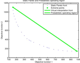
100 200 300 400 500 600 700 800 900 1000 0

200 400 600 800 1000 1200

Static Pareto and Probabilistic operating region

Objective function 1

Static Pareto front Extreme points Virtual interpolation front Probabilistic operating region

Figure 3: Operating Region for Example 1

Note that the extreme points in each figure correspond to the individual solutions to Problems (7) and belong to the orig-inal Pareto-optimal region. Observe that, the more evenly distributed the probability distribution is, the closer the cor-responding virtual operating point gets to the center of the virtual operating region, which is formed by the convex com-bination of theK extreme points. Observe also that the vir-tual operating points between the extreme points are always dominated by some point in the original Pareto-optimal re-gion. However, as we increase K, the Pareto front of the proposed probabilistic approach gets closer to that of the tra-ditional static formulation. One can see in Fig. 5 that the Pareto front of the proposed approach, withK=5 operating points, almost coincides with the Pareto front of the original formulation.

Finding a function that maps the Pareto front can be very involving. Hence, the classical methods that solve multiob-jective problems obtain a limited Pareto-optimal set and it is very sparse sometimes. In such problems, a probabilistic operation can be expand the operating region, providing an infinite number of solutions to choose from, and thus adding flexibility and additional trade-offs for the decision maker.

(9)

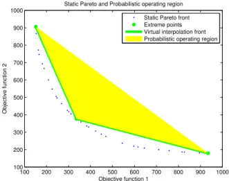
100 200 300 400 500 600 700 800 900 1000 100

200 300 400 500 600 700 800 900 1000

is Pareto-optimal within the proposed formulation. The com-putational time required to find the static Pareto front was 11.6070s, while the two points of the virtual interpolation front were found in 0.1930s.

For Example 2, we select a middle point in addition to the extreme points in thestaticPareto front to compose the oper-ating setOp. The resulting probabilistic operating region is depicted in Fig. 4. Note that the Pareto front of the pro-posed formulation gets closer to that of the static formu-lation. This illustrates that even a small subset of operat-ing points can render the performance of the probabilistic method almost equivalent to the performance of the classical approach. Moreover, as observed above, the range of possi-bilities for the decision maker to choose from increases dra-matically by applying the probabilistic approach. The com-putational time required to find the static Pareto front was 15.6160s, while the three points of the virtual interpolation front were found in 0.3480s.

For Example 3, we select five points to generate the proba-bilistic operating region. In this example, the virtual interpo-lation front is even closer the Pareto front than in Example 2. The results are depicted in Figure 5. Observe that, the more we increase the number of operating points inOp, the closer the probabilistic Pareto front gets to thestaticfront. Naturally, there is a compromise between the cardinality of the selected set of extreme points and the computational ef-fort needed to identify those points. It is worth noting that the proposed examples suggest that a modest number of op-erating points can result in a performance which closely ap-proximates that of the original static formulation, while pro-viding extra flexibility and additional trade-offs for the deci-sion making process. The computational time required to the static Pareto front was 9.4340s, while the five points of the

virtual interpolation front were found in 0.4830s.

200 300 400 500 600 700 800 900 1000 1100 1200 100

200 300 400 500 600 700 800 900 1000 1100

Observe also that one can assign to the probabilistic operat-ing setOpthe whole classical Pareto-optimal set. Hence, it is not difficult to see that the proposed probabilistic approach is a generalization of the static MOP formulation.

For Example 4, we select ten points to generate the proba-bilistic operating region. The results are depicted in Figure 6. The blue points form Pareto front and they were divided into layers to better represent the frontier uncover the virtual in-terpolation front, which is green, while the operating region is yellow. Note that the Pareto front of the proposed formu-lation gets very close to that of thestaticformulation. The computational time required to find the static Pareto front was 28.7020s, while the ten points of the virtual interpola-tion were found in 4.4490s.

For Example 5, we select ten points to generate the proba-bilistic operating region. The results are depicted in Figure 7. The computational time required to reach find the static Pareto front was 101.8310s, while the ten points of the vir-tual interpolation were found in17.3220s.

6 CONCLUDING REMARKS

(10)

0 2000 4000

0 500 1000 1500 2000 2500 3000 0 500 1000 1500 2000 2500 3000

Objective function 2 Objective function 1

(a) Left side

0 500 1000 1500 2000 2500 3000 0 2000

4000 0

500 1000 1500 2000 2500 3000

Objective function 2 Static Pareto and Probabilistic operating region

(b) Right side

0 2000 4000 6000

0 1000 2000 3000 4000 5000 6000 0

1000 2000 3000 4000 5000

(a) Left side

0 ₁₀₀₀

2000 3000 4000 5000 0 2000

4000 6000 0

1000 2000 3000 4000 5000

(b) Right side

The proposed approach can add flexibility to the decision maker by creating a new, expanded set ofvirtualoperating points, each corresponding to a given probability distribu-tion. Moreover, a careful selection of a finite set of operating points can render the probabilistic Pareto-optimal region al-most equivalent to the original MOP Pareto front. This limits the number of operating points, rendering the long term oper-ation more efficient and specialized, while also maintaining the performance requirements.

One possible drawback of the method is that, although it can limit the number of operating points to be found in the staticPareto front, the cost of finding each such point still depends on the problem at hand, and one may be forced to seek approximate solutions in the case of NP-hard and/or large-scale problems. Future research directions involve con-trasting the proposed method with purely stochastic formu-lations, such as multi-objective Markov decision processes, as well as studying the effect of the proposed formulation in non-convex MOP problems. A conjecture that remains to be verified is that the probabilistic Pareto front on the latter

problems can, in fact, dominate some solutions in the static Pareto front.

REFERENCES

ABIDO, M. A. (2006). Multiobjective evolutionary al-gorithms for electric power dispatch problem, IEEE Transactions on Evolutionary Computation10(3): 315– 329.

AMORIM, E. A., ROMERO, R. and MANTOVANI, J. R. S. (2009). Fluxo de potência ótimo descentralizado uti-lizando algoritmos evolutivos multiobjetivo, Controle & Automação20: 217–232.

ATHANS, A. and GEERING, H. P. (1973). Necessary and sufficient conditions for differenciable nonscalar-valued functions to attain extrema, IEEE Transaction on Automatic Control18(2): 132–139.

(11)

algo-rithms, second edn, Jonh Wiley & Sons, New York, USA.

BRÉMAUD, P. (1999).Gibbs fields, monte carlo simulation, and queues, Springer-Verlag, New York, USA.

CARDOSO, R. T. N., da CRUZ, A. R., WANNER, E. F. and TAKAHASHI, R. H. C. (2009). Multi-objective evo-lutionary optimization of biological pest control with impulsive dynamic in soybeans crops,Bulletin of Math-ematical Biology71: 1463–1481.

CHANKONG, V. and HAIMES, Y. Y. (1983). Multiobjec-tive decision making: Theory and Methodology, Vol. 8 of North Hollando series in system science and engi-neering, North Holland, New York, USA.

CHINCHULUUN, A. and PARDALOS, P. M. (2007). A sur-vey of recent developments in multiobjective optimiza-tion,Annals of Operational Research154: 29–50.

COELLO, C. A. C., VAN VELDHUIZEN, D. A. and LAM-ONT, G. B. (2002). Evolutionary algorithms for solv-ing multi-objective problems, Kluwer Academic Pub-lishers, New York. ISBN 0-3064-6762-3.

DEB, K. (2001). Multi-objective optimization using evolu-tionary algorithms, John Wiley & Sons, LTD, Chich-ester, UK.

DIAS, J., CAPTIVO, M. E. and CLÍMACO, J. (2008). A memetic algorithm for multi-objective dynamic loca-tion problems,Journal of Global Optimization42: 221– 253.

EHRGOTT, M., PUERTO, J. and RODRÍGUEZ-CHÍA, A. M. (2007). Primal-dual simplex method for multi-objective linear programming,Journal of Optimization Theory and Applications134(3): 483–497.

ESOGBUE, A. O., SONG, Q. and YOUNG, D. (2006). Non-euler-lagrangian pareto-optimality conditions for dy-namic multiple criterion decision problems, Mathemat-ical Methods of Operations Research63(3): 525–542.

EVERSON, R. M. and FIELDSEND, J. E. (2006). Multiob-jective optimization of safety related systems: An ap-plication to short-term conflict alert,IEEE Transactions on Evolutionary Computation10(2): 187–198.

FERNÁNDEZ, E. and PUERTO, J. (2003). Multiobjective solution of the uncapacitated plant location problem, European Journal of Operational Research145: 509– 529.

INSUA, D. R. (1990). Sensitivity analysis in multiobjective decision making,inM. BECKMANN and W. KRELLE (eds), Lecture Notes in Economics and Mathematical Systems, Vol. 347, Springer-Verlag, Berlin, Germany.

KEENEY, R. L. and RAIFFA, H. (1976).Decisions with mu-tiples objectives: preferences and calue trade-off, Wi-ley, New York, USA.

KIM, I. Y. and de WECK, O. L. (2006). Adaptive weighted sum method for multiobjective optimization: a new method for pareto front generation,Structural and Mul-tidisciplinary Optimization31(2): 105–116.

MARLER, R. T. and ARORA, J. S. (2004). Survey of multi-objective optimization methods for engineering, Struc-tural and Multidisciplinary Optimization 26(6): 369– 395.

NEMHAUSER, G. L. and WOSLEY, L. A. (1999). Inte-ger and combinatorial optimization, Wiley, New York, USA.

PARETO, V. (1897a).Cours d’economique politique, Vol. I, Macmillan, Paris, FR.

PARETO, V. (1897b). Le cours d’economique politique, Vol. II, Macmillan, London, UK.

REID, R. W. and CITRON, S. J. (1971). On noninferior per-formance index vectors,Journal of Optimization The-ory and Applications7(1): 11–28.

ROSS, S. M. (2009). Introduction to probability and statis-tics for engineers and scientists, fourth edn, Academic Press, New York, USA.

SAKAWA, M. and YAUCHI, K. (1998). Coevolutionary ge-netic algorithms for nonconvex nonlinear programming problems: Revised genocop iii, Cybernetics and Sys-tems29(8): 885–899.

SALUKVADZE, M. (1974). On the existence of solutions in problems of optimization under vector-valued cri-teri,Journal of Optimization Theory and Applications

13(2): 203–217.

STADLER, W. (1979). a survey of multicriteria optimiza-tion ot the vector maximum problem, part i: 1776-1960,Journal of Optimization Theory and Applications

29(1): 1–52.

TRALHÃO, L., COUTINHO-RODRIGUES, J. and ALÇADA-ALMEIDA, L. (2010). A multiobjective modeling approach to locate multi-compartment containers for urban-sorted waste,Waste Management

30: 2418–2429.