doi: 10.1590/0101-7438.2016.036.02.0241
A NEW MATHEMATICAL MODEL FOR THE WORKOVER RIG SCHEDULING PROBLEM
Miguel P´erez, Fabricio Oliveira and Silvio Hamacher
*Received February 5, 2016 / Accepted June 4, 2016
ABSTRACT.One of the most important activities in the oil and gas industry is the intervention in wells for maintenance services, which is necessary to ensure the constant production of oil. These interventions are carried out by workover rigs. Thus, the Workover Rig Scheduling Problem (WRSP) consists of finding the best schedule to service the wells while considering the limited number of rigs with the objective of minimizing the total production loss. In this study, a 0-1 integer linear programming model capable of effi-ciently solving the WRSP with a homogeneous fleet of rigs is proposed. Computational experiments were carried out using instances based on real cases in Brazil to compare the results obtained by the proposed model with the results reported by other methods. The proposed model was capable of solving all instances considered in a reduced computational time, including the large instances for which only approximate solutions were presently known.
Keywords: oil production, workover rigs, 0-1 Integer Linear Programming.
1 INTRODUCTION
Usually for oil wells to operate at onshore fields, it is necessary to pump fluids so that the oil reaches the surface. Fluid lift can be carried out by various artificial techniques, such as me-chanical pumping, progressive cavity pumping, gas lift and others. As a result, it is necessary to install equipment that works next to the well pumping the fluids. Over time, wells and pieces of equipment require maintenance services (called workover), such as cleaning, reinstatement, stimulation and others, all of which aim to maintain the production or to improve the productivity of the well. The interventions in the wells are performed by workover rigs.
The rigs are limited and scarce resources with high operational costs, and there are a large number of wells that demand maintenance services. Therefore, a service schedule should be defined for the wells. The construction of the schedule should be based on factors such as the oil production of the well, the type of service that needs to be performed and the available time window to carry
*Corresponding author.
out the service. Waiting for service can cause the wells to become inactive, which causes major production losses (Aloise et al., 2006).
The problem of intervention in wells for maintenance services is one of the most important activities in the oil and gas industry. Thus, providing optimal solutions is an issue that can lead to thousands of dollars in savings due to the reduction of the oil production loss as it can be confirmed in the works of Costa (2005) and Aloise et al. (2006).
Thus, the Workover Rig Scheduling Problem (WRSP) consists of establishing the schedule of the well service while considering the limited number of available rigs and minimizing the total production loss due to waiting for maintenance services in a planning horizon. The WRSP can be classified as a particular case of the scheduling problem, where the maintenance services represent a set of tasks and the rigs represent a set of parallel machines and that aim to minimize the total weighted tardiness (Colin & Shimizu, 2000; Valente & Alves, 2003). This problem is of a combinatorial nature and belongs to the NP-hard class (Du & Leung, 1990). For scheduling problems can be found a vast amount of literature addressing its classic form and extensions.
The present paper proposes a 0-1 integer linear programming model to efficiently solve the WRSP. This mathematical model extends the mathematical model proposed by Costa & Fer-reira Filho (2004). A reformulation and decomposition procedure are developed to formulate the WRSP using a smaller number of decision variables and constraints, allowing to solve large instances.
The proposed model was tested in instances generated by Costa (2005) from real cases of an oil production field in Brazil. In the literature, 25 instances are available; optimum values are known for 10 of them, as reported by Pacheco, Dias Filho & Ribeiro (2009) by using the CPLEX 12.1 solver. These authors were not able to solve the remaining instances due to their great com-plexity, and only approximate solutions reported by some heuristics and metaheuristics for those instances are known.
Thus, there are two main contributions in this paper. First, this paper describes the development of a new formulation for the problem in question, which proved to be more efficient than the methods available in the literature. The second contribution is the generation of optimum solu-tions for the instances of Costa (2005), which were not known in the literature until now.
This study is structured as follows: A review of the literature is presented in Section 2. The WRSP is formulated and the proposed model is developed in Section 3. The computational re-sults are analyzed in Section 4, and the proposed model is compared with the methods available in the literature. Finally, conclusions and proposals for future work are presented in Section 5.
2 LITERATURE REVIEW
is considered significant. According to Gouvˆea, Goldbarg & Costa (2002), using the scheduling approach is appropriate when the times required to move the rigs between the wells are on the order of minutes or hours and the rig intervention time is on the order of days or weeks.
Among the applications that addressed the approach of routing and scheduling, the following applications stand out: Paiva (1997); Paiva, Schiozer & Bordalo (2000); Aloise et al. (2006); Ribeiro, Laporte & Mauri (2012); Ribeiro, Desaulniers & Desrosiers (2012); Duhamel, Santos & Guedes (2012); Bassi, Ferreira Filho & Bahiense (2012); Ribeiro et al. (2014); Monemi et al. (2015).
Paiva (1997) and Paiva, Schiozer & Bordalo (2000) presented a study employing a reservoir simulator to analyze the monetary influence due to well shutdown when a failure is detected on the present value of the production curve. Aloise et al. (2006) proposed a Variable Neigh-borhood Search (VNS) heuristic. The latter used a constructive heuristic to generate initial so-lutions, defining nine different neighborhoods to search for better solutions. Ribeiro, Laporte & Mauri (2012) applied the Clustering Search (CS) and Adaptive Large Neighborhood Search (ALNS) heuristics, comparing the results with the Iterated Local Search (ILS) proposed by Neves (2007). Among the 3 heuristics, the ALNS showed the best results. Ribeiro, Desaulniers & Desrosiers (2012) presented a mathematical model for this problem and a Branch Price and Cut (BPC) algorithm. The BPC algorithm consists of obtaining a strong relaxation of the mathe-matical model by incorporating column generation in the Branch & Cut method. The generation of columns adds cuts to determine the lower bounds of the search tree. To test the algorithm, ran-dom instances were generated from the instances proposed by Neves (2007). Duhamel, Santos & Guedes (2012) proposed 3 mixed integer linear programming models. The first is an improve-ment of the model proposed by Aloise et al. (2006), the second is based on the open vehicle routing model and the third is based on the set covering model incorporating the column genera-tion strategy to find the optimal linear relaxagenera-tion solugenera-tion. The best results were obtained by the third mathematical model, achieving optimal values for medium-sized instances. Bassi, Ferreira Filho & Bahiense (2012) presented the first study dealing with uncertain data for this approach. A simulation-optimization method was developed to generate expected solutions. The simulation stage consists of performing a random sampling of uncertain data to be solved in the optimization stage. In the optimization stage, a greedy algorithm and a Greedy Randomized Adaptive Search Procedure (GRASP) metaheuristic were used. Ribeiro et al. (2014) presented a BPC heuristic and a Hybrid Genetic Algorithm (HGA). Monemi et al. (2015) proposed a mixed integer linear programming model. The solution method begins with a hyper-heuristic and this result is used to generate columns for BPC algorithm. The numerical experiments were performed in disturbed data from an onshore field in Brazil. The method is able to solve small instances.
Smith (1956) showed that for the case of one rig, the optimal schedule is obtained when the wells are ordered in decreasing values ofPi/di, called Natural Order, wherePi is the production loss in welli per day and di is the duration of the intervention in welli. Brennan, Barnes &
Knapp (1977) showed a lower bound for WRSP with N rigs and J wells based on the papers published by Smith (1956) and Eastman, Even & Isaacs (1964). Costa & Ferreira Filho (2004) proposed a mathematical model and a heuristic based on the Natural Order. Costa (2005) im-plemented a GRASP metaheuristic, and they constructed instances based on real cases from an onshore field in Brazil. Costa & Ferreira Filho (2005) proposed a Dynamic Assembly Heuris-tic (DAH) that allocates the services sequentially according to the criterion described in Costa & Ferreira Filho (2004), testing all of the possibilities for adding a new service before and after those already programmed and dynamically allocating the services to the rigs with the purpose of improving the solution. Alves & Ferreira Filho (2006) proposed a Genetic Algorithm (GA) in which the solutions (chromosomes) represent a vector of wells that will be distributed to the rigs. The crossover operator that was used was the uniform order crossover, and the mutation operator was the random swap of two positions in the well vector. Oliveira et al. (2007) presented an evolutionary algorithm based on the Scatter Search (SS) metaheuristic that operates over a population of solutions and employs procedures to combine those solutions with the goal of gen-erating better solutions. Instead of randomly exploring solutions like the GA, the SS extensively explores predetermined regions in each new iteration. Pacheco, Dias Filho & Ribeiro (2009) pro-posed a Bubble Swap (BS) heuristic. This heuristic is constructed in two stages. In the first stage, a feasible solution is generated through the heuristic proposed by Costa & Ferreira Filho (2004), and the second stage consists of performing a swap of wells in the same rig and between dif-ferent rigs. Douro & Lorenzoni (2009) presented a GA with a 2-opt local search technique. The solutions (chromosomes) are represented by a well vector that is distributed to the rigs. The sin-gle point was used as the crossover operator, and the simple inversion mutation operator was used as the mutation operator. Pacheco, Ribeiro & Mauri (2010) presented a GRASP with Path-Relinking (PR) as an intensification strategy, exploring the paths that connect the elite solutions to search for better solutions. Pacheco (2011) presented a Memetic Algorithm (MA) metaheuris-tic where a strategy based on the Natural Order is applied on the chromosomes. Ribeiro, Mauri & Lorena (2011) applied a Simulated Annealing (SA) with three different moves to compose the neighborhood structure.
3 PROBLEM FORMULATION
The WRSP is formulated as follows: a set of available rigsm =1,2, . . . ,N and a set of wells
i = 1,2, . . . ,J that require maintenance services, in which each welli is associated with an intervention timedi; a time window in the range [ei,li] in which it can be serviced; and a value of production lossPi, which indicates how much that well will not produce (in units of volume
per unit of time). The execution of each intervention in a well requires that a rig is selected. Thus, the WRSP consists of determining the service schedule for the wells by the rigs with the objective of minimizing the total production loss due to the time that the wells waited for maintenance service in a planning horizon.
The assumptions are as follows:
• The fleet of rigs is considered homogenous.
• The travel times between each pair of wells are not considered because they are not signif-icant compared to the intervention times.
• The assembly and disassembly times are included in the intervention times.
• Each rig operates without idle time until all wells allocated to the rig have been serviced.
• Once the intervention is started, it cannot be interrupted.
The following notation is used to formulate the WRSP:
J number of wells,i,j = {1,2, . . . ,J}
N number of rigs,m= {1,2, . . . ,N}
T planning horizon,t,h= {1,2, . . . ,T}
di duration of the intervention in welli Pi production loss in welliper unit time
[ei,li] time window, whereei is the earliest start time for the intervention in
welliandli is the latest finish time for the intervention in welli
The decision variables are defined as follows:
Simt binary variable that takes on the value of 1 if rigmstarts the service in
welliat timet; otherwise, it takes on the value 0
Cimt binary variable that takes on the value of 1 if rigmfinishes the service
in welliat timet; otherwise, it takes on the value 0
Ximt binary variable that takes on the value of 1 if rigmis performing the service in welliat timet; otherwise, it takes on the value 0
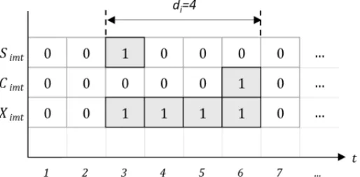
Figure 1 illustrates the representation of the decision variables. Suppose that a certain interven-tionistarts att =3(Sim3=1), if the duration of the intervention is 4 time units(di =4), then
the finish of the intervention will be att =6(Cim6 =1), such that the total time that requires a rig in a well is exactlydi =4. That is, the intervention occurs in the range 3≤t ≤6(Xim3= Xim4 = Xim5 = Xim6 = 1, mN=1
T
Figure 1– An example of a representation of decision variables.
3.1 Original Mathematical Model
Costa & Ferreira Filho (2004) proposed a 0-1 integer linear programming model, here called the Original Mathematical Model (OMM) for the WRSP, which is formulated with the variable
Simt and represented as:
(OMM) Minimize
J
i=1 N
m=1 T
t=1
(t+di −ei)PiSimt (1)
Subject to:
N
m=1 T
t=1
Simt =1 ∀i (2)
J
i=1
Simt ≤1 ∀m,t (3)
Simt +Sj mh≤1 ∀i,j,m,t,h|i= jandt ≤h≤t+di−1 (4)
Simt ∈ {0,1} ∀i,m,t|ei ≤t ≤li−di+1 (5)
In this mathematical model, the objective function (1) represents minimizing the total production loss. Constraint (2) ensures that the start of the intervention in each well occurs only once by a rig at a specific time. Constraint (3) ensures that a rig starts at most one intervention at a specific time. Constraint (4) ensures that there is no interference between the services in the wells that use the same rig; that is, no well jcan be serviced in the range[t,t+di−1]by rigmif welliis
being serviced in that range by the same rigm. Constraint (5) defines the domain of the decision variables and ensures that the start of the interventions in the wells is within the time window.
3.2 Reformulated Mathematical Model
the variablesSimt,CimtandXimt. With the inclusion of these variables, the WRSP is formulated
as follows:
Minimize
J
i=1 N
m=1 T
t=1
(t+di−ei)PiSimt (6)
Subject to:
N
m=1 T
t=1
Simt =1 ∀i (7)
J
i=1
Simt ≤1 ∀m,t (8)
Simt =0 ∀i,m,t|t<eiort >li−di+1 (9)
N
m=1 T
t=1
Cimt =1 ∀i (10)
J
i=1
Cimt ≤1 ∀m,t (11)
Cimt =0 ∀i,m,t|t<ei+di−1 ort>li (12)
Cimt =Sim,t−di+1 ∀i,m,t|t ≥di (13)
Ximt = t
h=1 Simh−
t−1
h=1
Cimh ∀i,m,t (14)
J
i=1
Ximt ≤1 ∀m,t (15)
Simt,Cimt,Ximt∈ {0,1} ∀i,m,t (16)
In this formulation, the variableCimt depends ofSimtand the variableXimtdepends on the choice
ofSimtandCimt to be determined. Thus, constraint (13) can be replaced in constraint (14):
Ximt = t
h=1 Simh−
t−1
h=1
Sim,h−di+1 ∀i,m,t
This constraint can be further simplified as follows:
Ximt = t
h=t−di+1
Simh ∀i,m,t (17)
Equation (17) is equivalent to equation (14).
Equation (14), together with equation (15), ensures that there is no interference between the serviced wells that are allocated to a rig. Substituting equation (17) in equation (15) gives:
J
i=1 t
h=t−di+1
Simh≤1 ∀m,t
Finally, the previous mathematical model is formulated by substituting the variablesCimt and Ximtas a function of the variableSimt, so that the Constraints (10), (11) and (12) become
unnec-essary. The RMM is shown below:
(RMM) Minimize
J
i=1 N
m=1 T
t=1
(t+di−ei)PiSimt (18)
Subject to:
N
m=1 T
t=1
Simt =1 ∀i (19)
J
i=1 t
h=t−di+1
Simh≤1 ∀m,t (20)
Simt∈ {0,1} ∀i,m,t|ei ≤t ≤li−di+1 (21)
3.3 Decomposed Mathematical Model
In this paper, the proposed mathematical model is presented as a Decomposed Mathematical Model (DMM), which is formulated from the RMM with a new decision variable:
Sit′ =
N
m=1
Simt ∀i,t
where:
Sit′ binary variable that takes on the value of 1 if the service in welli starts at timet; otherwise, it takes on the value 0
The variableSit′ could be used to replace the variableSimt directly in the RMM except for
con-straint (20). Thus, applying the sum for allm in constraint (20) and assuming that the rigs are homogenous, the following applies:
N
m=1 J
i=1 t
h=t−di+1 Simh≤
N
m=1 1 ∀t
J
i=1 t
h=t−di+1
Sih′ ≤ N ∀t
Given that a maximum ofN rigs perform the maintenance services in the wells at the same time, this constraint ensures that a maximum of Ninterventions are performed at a specific time and that there is no interference between the wells.
Thus, substituting the variable Simt as a function of the variable Sit′ in the RMM, a DMM is obtained, which determines the optimum start of the interventions in the wells as shown below:
(DMM) Minimize
J
i=1 T
t=1
(t+di−ei)PiSit′ (22)
Subject to:
T
t=1
Sit′ =1 ∀i (23)
J
i=1 t
h=t−di+1
Sih′ ≤N ∀t (24)
Sit′ ∈ {0,1} ∀i,t|ei ≤t ≤li −di+1 (25)
From the DMM, the optimum solutions Sit′∗ are obtained. These solutions will be used to de-termine the allocation of the wells to the rigs throughout the planning horizon. This allocation can be achieved by constructing a simple algorithm that allocates the wells to the rigs consecu-tively following the service order in time. Another way to determine this allocation is to solve the RMM, redefining the domain of the variableSimt depending on the optimal solutionsSit′∗. The suitability of the RMM for this purpose is shown next.
(RMM’) Minimize
J
i=1 N
m=1 T
t=1
(t+di−ei)PiSimt (26)
Subject to:
N
m=1 T
t=1
Simt =1 ∀i (27)
J
i=1 t
h=t−di+1
Simh≤1 ∀m,t (28)
Simt ∈ {0,1} ∀i,m,t|S′it
∗
=1 (29)
In this mathematical model, constraints (27) and (28) and the objective function (26) have a similar interpretation to constraints (19) and (20) and the objective function (18) of the RMM, respectively. Constraint (29) defines the constrained domain of the decision variable Simt and
ensures that the start of interventions in the wells are exactly the values foundS′
it
∗
, that is, only in the cases whereSit′∗ =1, the variableSimtwill be defined to determine the allocation of the
wells to the rigs.
3.4 Comparison between the OMM, the RMM and the DMM
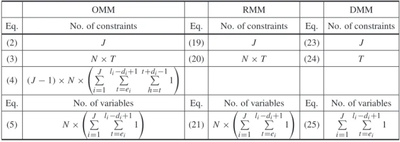
Table 1 shows the total number of constraints and variables used in the OMM, RMM and DMM.
Table 1– Comparison of the total number of constraints and variables in the OMM, RMM and DMM.
OMM RMM DMM
Eq. No. of constraints Eq. No. of constraints Eq. No. of constraints
(2) J (19) J (23) J
(3) N×T (20) N×T (24) T
(4) (J−1)×N×
J i=1
li−di+1 t=ei
t+di−1 h=t
1
Eq. No. of variables Eq. No. of variables Eq. No. of variables
(5) N×
J i=1
li−di+1 t=ei
1
(21) N×
J i=1
li−di+1 t=ei
1
(25)
J i=1
li−di+1 t=ei
The RMM and the DMM are formulated with fewer constraints compared to that of the OMM, and constraint (4) of the latter generates the most constraints. While the OMM uses the variables
Simt andSj mhin constraints (3) and (4), the RMM and the DMM do not use the index jof the
formulation and use the variableSimhin constraint (20) and the variableSih′ in constraint (24), that is, they use fewer constraints. The same number of variables is used in the OMM and the RMM, and fewer are used in the DMM compared to them because it is a mathematical model that does not consider the problem of allocating wells to rigs.
4 COMPUTATIONAL RESULTS
To evaluate the performance of the DMM, this model were compared to the OMM. The instances of Costa (2005) were used. These samples consist of 25 instances that have 25, 50, 75, 100 and 125 wells with 2, 4, 6, 8 and 10 rigs, generated from real cases in Brazil, where the values of production loss(Pi)are in units of(m3/day)/10, and the values of the intervention time(di)are
in units of half of a day (12 hrs).
The mathematical models were implemented in the AIMMS 3.14 software using the CPLEX 12.4 solver and run on a computer equipped with an Intel Core i7-3960X processor with 3.3 GHz and 64 GB of RAM.
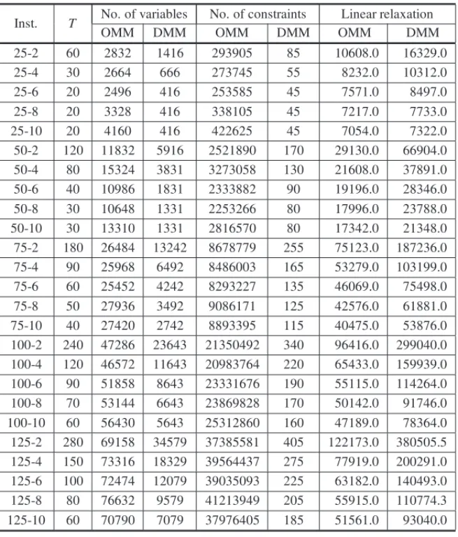
Next, a preliminary analysis was performed, and Table 2 shows the planning horizon(T)for each processed instance, the number of variables, the number of constraints and the optimal values of the objective function obtained via linear relaxation for the OMM and DMM.
Table 2 shows the significant differences between the number of constraints of the OMM com-pared to of the DMM, similar to Table 1. Furthermore, according to the values of the linear relaxation, the DMM obtained the best lower bounds for the different instances, with a mean difference of 40% relative to the OMM. This result supports the statement that such formulation is stronger concerning the use of methods based on linear relaxation (such as methods based on branch-and-bound strategies), which in turn implies that they obtain optimum solutions in a more efficient manner.
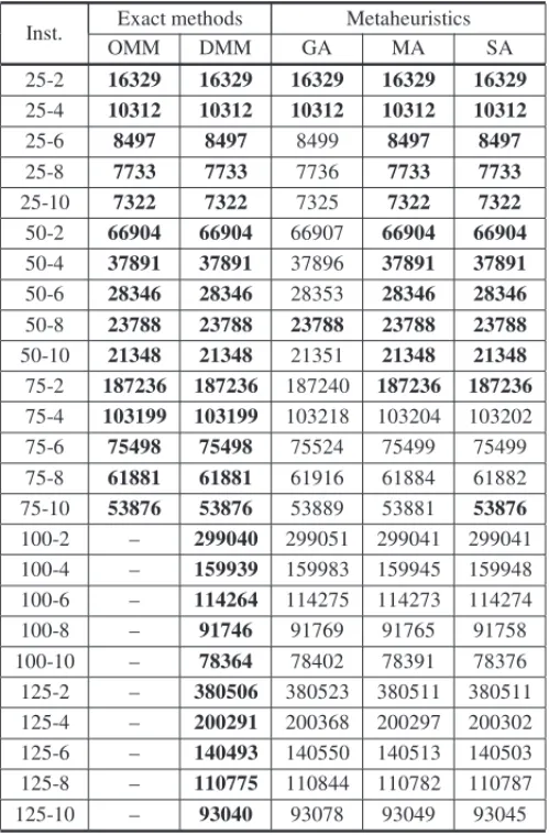
Table 3 presents the results of the objective function obtained for the WRSP by the OMM and DMM exact methods and then compares the results with other methods available in the literature. In this table, those methods that obtained the best results are shown: GA (Douro & Lorenzoni, 2009), MA (Pacheco, 2011) and SA (Ribeiro, Mauri & Lorena, 2011). As the solver stopping criteria, a GAP of 0% and a run time limit of 300 s were established to solve the OMM and DMM.
Table 2– Results of the linear relaxation applied to the OMM and DMM.
Inst. T No. of variables No. of constraints Linear relaxation
OMM DMM OMM DMM OMM DMM
25-2 60 2832 1416 293905 85 10608.0 16329.0 25-4 30 2664 666 273745 55 8232.0 10312.0
25-6 20 2496 416 253585 45 7571.0 8497.0
25-8 20 3328 416 338105 45 7217.0 7733.0
25-10 20 4160 416 422625 45 7054.0 7322.0 50-2 120 11832 5916 2521890 170 29130.0 66904.0 50-4 80 15324 3831 3273058 130 21608.0 37891.0 50-6 40 10986 1831 2333882 90 19196.0 28346.0 50-8 30 10648 1331 2253266 80 17996.0 23788.0 50-10 30 13310 1331 2816570 80 17342.0 21348.0 75-2 180 26484 13242 8678779 255 75123.0 187236.0 75-4 90 25968 6492 8486003 165 53279.0 103199.0 75-6 60 25452 4242 8293227 135 46069.0 75498.0 75-8 50 27936 3492 9086171 125 42576.0 61881.0 75-10 40 27420 2742 8893395 115 40475.0 53876.0 100-2 240 47286 23643 21350492 340 96416.0 299040.0 100-4 120 46572 11643 20983764 220 65433.0 159939.0 100-6 90 51858 8643 23331676 190 55115.0 114264.0 100-8 70 53144 6643 23869828 170 50142.0 91746.0 100-10 60 56430 5643 25312860 160 47189.0 78364.0 125-2 280 69158 34579 37385581 405 122173.0 380505.5 125-4 150 73316 18329 39564437 275 77919.0 200291.0 125-6 100 72474 12079 39035093 225 63182.0 140493.0 125-8 80 76632 9579 41213949 205 55915.0 110774.3 125-10 60 70790 7079 37976405 185 51561.0 93040.0
As a more modern computer was used here than in Pacheco, Dias Filho & Ribeiro (2009), it was possible to find solutions using the OMM for the instances with 75 wells.
A comparison between the results of the linear relaxation in Table 2 and the results of the exact methods in Table 3 shows that the DMM obtained lower bounds that are very close to the opti-mum value of the objective function, where the linear relaxation did not reach the optiopti-mum value of the problem in only two instances.
Regarding the metaheuristics, in general, the best results were obtained by the SA, but it was able to solve only two of the large instances optimally.
Table 3– Numerical results of the different methods that were employed.
Inst. Exact methods Metaheuristics
OMM DMM GA MA SA
25-2 16329 16329 16329 16329 16329
25-4 10312 10312 10312 10312 10312
25-6 8497 8497 8499 8497 8497
25-8 7733 7733 7736 7733 7733
25-10 7322 7322 7325 7322 7322
50-2 66904 66904 66907 66904 66904
50-4 37891 37891 37896 37891 37891
50-6 28346 28346 28353 28346 28346
50-8 23788 23788 23788 23788 23788
50-10 21348 21348 21351 21348 21348 75-2 187236 187236 187240 187236 187236 75-4 103199 103199 103218 103204 103202
75-6 75498 75498 75524 75499 75499
75-8 61881 61881 61916 61884 61882
75-10 53876 53876 53889 53881 53876 100-2 – 299040 299051 299041 299041 100-4 – 159939 159983 159945 159948 100-6 – 114264 114275 114273 114274 100-8 – 91746 91769 91765 91758 100-10 – 78364 78402 78391 78376 125-2 – 380506 380523 380511 380511 125-4 – 200291 200368 200297 200302 125-6 – 140493 140550 140513 140503 125-8 – 110775 110844 110782 110787 125-10 – 93040 93078 93049 93045
Table 4 shows that the DMM can solve the WRSP more efficiently than the OMM. For example, in the instances with 75 wells, the OMM needed 109.9 s on average (considering the 5 instances of 75 wells), while the DMM needed 0.4 s on average; that is, a remarkable reduction of the consumed time. In the instances with 25 and 50 wells, the DMM also notably reduced the time consumed compared to that of the OMM. In the large instances with 100 and 125 wells, the DMM needed 1.3 s and 2.3 s on average, respectively. The DMM required a computational time of less than 7 s to solve each instance, requiring 0.8 s on average. The proposed model has a lower mean time than that of the OMM and is the most efficient to solve the WRSP according to the computational results.
Table 4– Computational times (s).
Inst. Exact methods Metaheuristics OMM DMM GAa MAb SAc
25-2 3.3 0.0 4.0 2.4 4.2
25-4 3.0 0.0 5.0 3.5 4.6
25-6 3.1 0.0 2.0 3.9 5.7
25-8 4.3 0.0 1.0 5.1 7.0
25-10 5.4 0.0 1.0 6.9 8.3
50-2 30.2 0.3 14.0 4.1 6.7 50-4 36.1 0.2 15.0 6.8 6.7 50-6 26.0 0.0 5.0 7.9 7.7 50-8 25.9 0.0 16.0 10.9 8.5 50-10 32.6 0.0 10.0 14.0 10.4
75-2 122.7 1.4 36.0 5.9 9.2 75-4 105.1 0.4 27.0 7.5 8.4 75-6 98.2 0.2 25.0 12.6 9.6 75-8 111.2 0.1 18.0 16.8 10.6 75-10 112.5 0.1 29.0 22.6 11.9 100-2 – 3.8 61.0 17.6 11.9 100-4 – 1.5 48.0 10.4 10.3 100-6 – 0.5 136.0 15.1 11.1 100-8 – 0.5 141.0 20.7 12.9 100-10 – 0.3 58.0 28.2 13.8 125-2 – 6.2 146.0 10.5 14.6 125-4 – 3.3 60.0 12.2 12.1 125-6 – 0.9 84.0 19.4 12.7 125-8 – 0.8 66.0 26.0 14.2 125-10 – 0.5 164.0 34.5 15.7 Average 49.5 0.8 46.9 13.0 10.0
aComputer used Pentium IV 2.0 GHz processor with 480 MB of RAM.
bComputer used Pentium Core i3 2.13 GHz processor with 4 GB of RAM.
cComputer used AMD Athlon 64 3500 2.2 GHz processor with 1 GB of RAM.
the justification that, in general, the metaheuristics should perform several replications to ensure the robustness of the obtained solution, in addition to the time spent with previous experiments required to adjust the execution parameters.
5 CONCLUSIONS AND FUTURE WORKS
by inactive wells waiting for maintenance services. Because it is an NP-hard problem, the diffi-culty in solving the WRSP has resulted in various heuristics and metaheuristics in the literature. Although the heuristics and metaheuristics can obtain approximate solutions, they are not ca-pable of obtaining optimal solutions for large instances (e.g., large numbers of wells or rigs). Thus, to efficiently solve the WRSP, a 0-1 integer linear programming model was proposed. This mathematical model (DMM) extends the mathematical model proposed by Costa & Fer-reira Filho (2004) and proved to be more efficient in the computational experiments that were carried out.
The DMM was tested in instances based on real cases in Brazil and compared to various methods in the literature. The computational results showed that the DMM was able to solve all of the instances considered, including the large instances, and this model obtained optimum solutions, which were not known until now. Regarding the computational time, the DMM solved all of the instances in short times. Thus, the proposed model showed efficient performance in comparison to the other methods proposed to solve the WRSP.
The computational results corroborate the usefulness of the DMM as computational tool to solve real problems, with various numbers of wells and different rig fleet sizes for an established planning horizon. Consequently, DMM can be used by companies dedicated to planning in-terventions in wells or other analogous services, carrying out the planning quickly and reliably, reducing errors in the service schedule and improving the decision making capacity.
In future works, it is desirable to extend the proposed formulation to address the Workover Rig Routing Problem and the Rig Fleet Sizing Problem. Furthermore, due to the variations in the intervention times of the rigs and other uncertainties in the operations, it is desirable to apply techniques that are able to address the uncertain characteristics of the problem of intervention in wells.
Another important point is the generation of instances, given that there is only one group of instances available in the literature that were randomly built from an oil production field. There-fore, it is necessary to generate a new group of instances to address the problem of intervention in wells.
Finally, it would be important to test the formulations in offshore fields, which are generally more complex than onshore fields.
REFERENCES
[1] ALOISEDJ, ALOISED, ROCHACTM, RIBEIROCC, RIBEIROJC & MOURALSS. 2006. Schedul-ing workover rigs for onshore oil production.Discrete Applied Mathematics,154(5): 695–702.
[3] BASSIHV, FERREIRAFILHOVJM & BAHIENSEL. 2012. Planning and scheduling a fleet of rigs using simulation-optimization.Computers & Industrial Engineering,63(4): 1074–1088.
[4] BRENNANJJ, BARNESJW & KNAPPRM. 1977. Scheduling a backlog of oil well workovers. Jour-nal of Petroleum Technology,29(12): 1651–1653.
[5] COLINE & SHIMIZUT. 2000. Algoritmo de programac¸˜ao de m´aquinas individuais com penalidades distintas de adiantamento e atraso (Algorithm for machine scheduling with earliness and tardiness penalties).Pesquisa Operacional,20(1): 19–30.
[6] COSTA LR. 2005. Soluc¸˜oes para o problema de otimizac¸˜ao de itiner´ario de sondas (Solving the workover rig itinerary problem). Master Thesis, UFRJ, Rio de Janeiro, RJ, Brazil.
[7] COSTALR & FERREIRAFILHOVJM. 2004. Uma heur´ıstica para o problema do planejamento de itiner´arios de sondas em intervenc¸ ˜oes de poc¸os de petr´oleo (A heuristic for workover rig itinerary problem in oil wells).Proceedings of the XXXVI SBPO – Brazilian Symposium on Operations Re-search, S˜ao Jo˜ao Del Rei, MG, Brazil.
[8] COSTALR & FERREIRAFILHOVJM. 2005. Uma heur´ıstica de montagem dinˆamica para o prob-lema de otimizac¸˜ao de itiner´arios de sondas (A heuristic of dynamic mounting for the workover rig itinerary problem).Proceedings of the XXXVII SBPO – Brazilian Symposium on Operations Research, Gramado, RS, Brazil.
[9] DOURORF & LORENZONILL. 2009. Um algoritmo gen´etico-2opt aplicado ao problema de oti-mizac¸˜ao de itiner´ario de sondas de produc¸˜ao terrestre (A genetic-2opt algorithm applied to onshore workover rig itinerary problem).Proceedings of the XLI SBPO – Brazilian Symposium on Operations Research, Porto Seguro, BA, Brazil.
[10] DUJ & LEUNGJYT. 1990. Minimizing total tardiness on one machine is NP-hard.Mathematics of Operations Research,15(3): 483–495.
[11] DUHAMELC, SANTOSAC & GUEDESLM. 2012. Models and hybrid methods for the onshore wells maintenance problem.Computers & Operations Research,39(12): 2944–2953.
[12] EASTMANWL, EVENS & ISAACSIM. 1964. Bounds for the optimal scheduling ofnjobs onm processors.Management Science,11(2): 268–279.
[13] GOUVEAˆ EF, GOLDBARGMC & COSTAWE. 2002. Algoritmos evolucion´arios na soluc¸˜ao do pro-blema de otimizac¸˜ao do emprego de sondas de produc¸˜ao em poc¸os de petr´oleo (Evolutionary algo-rithms for solving the rig optimization problem in oil wells).Proceedings of the XXXIV SBPO – Brazilian Symposium on Operations Research, Rio de Janeiro, RJ, Brazil.
[14] MONEMIRN, DANACHK, KHALILW, GELAREHS, LIMAJRFC & ALOISEDJ. 2015. Solution methods for scheduling of heterogeneous parallel machines applied to the workover rig problem. Expert Systems with Applications,42(9): 4493–4505.
[15] NEVES TA. 2007. Heur´ısticas com mem´orias adaptativas aplicadas ao problema de roteamento e scheduling de sondas de manutenc¸˜ao (Heuristics with adaptive memory applied to the workover rig routing and scheduling problem). Master Thesis, UFF, Niter´oi, RJ, Brazil.
[17] PACHECOAVF. 2011. M´etodos de soluc¸˜ao para o problema da alocac¸˜ao de sondas a poc¸os de petr´oleo (Methods for solving the workover rig scheduling problem in oil wells). Graduate Thesis, UFES, S˜ao Mateus, ES, Brazil.
[18] PACHECOAVF, DIAS FILHO ACT & RIBEIRO GM. 2009. Uma heur´ıstica para o problema da alocac¸˜ao de sondas de produc¸˜ao em poc¸os de petr´oleo (A heuristic for the workover rig scheduling problem in oil wells).Proceedings of the XXIX ENEGEP – National Production Engineering Meeting, Salvador, BA, Brazil.
[19] PACHECOAVF, RIBEIROGM & MAURIGR. 2010. A GRASP with path-relinking for the workover rig scheduling problem.International Journal of Natural Computing Research,1(2): 1–14.
[20] PAIVARO. 1997. Otimizac¸˜ao do itiner´ario de sondas de intervenc¸˜ao (Optimizing the itinerary of workover rigs). Master Thesis, UNICAMP, Campinas, SP, Brazil.
[21] PAIVARO, SCHIOZERDJ & BORDALOSN. 2000. Optimizing the itinerary of workover rigs. Pro-ceedings of 16th World Petroleum Congress, Calgary, AB, Canada.
[22] RIBEIROGM, DESAULNIERSG & DESROSIERSJA. 2012. Branch-Price-and-Cut Algorithm for the workover rig routing problem.Computers & Industrial Engineering,39(12): 3305–3315.
[23] RIBEIROGM, DESAULNIERSG, DESROSIERSJ, VIDALT & VIEIRABS. 2014. Efficient heuristics for the workover rig routing problem with a heterogeneous fleet and a finite horizon.Journal of Heuristics,20(6): 677–708.
[24] RIBEIRO GM, LAPORTE G & MAURIGR. 2012. A comparison of three metaheuristics for the workover rig routing problem.European Journal of Operational Research,220(1): 28–36.
[25] RIBEIROGM, MAURIGR & LORENALAM. 2011. A simple and robust simulated annealing algo-rithm for scheduling workover rigs on onshore oil fields.Computers & Industrial Engineering,60(4): 519–526.
[26] SMITHWE. 1956. Various optimizers for single-stage production.Naval Research Logistics Quar-terly,3(1-2): 59–66.
[27] VALENTE J & ALVES R. 2003. Efficient polynomial algorithms for special cases of weighted early/tardy scheduling with release dates and a common due date.Pesquisa Operacional,23(3): 443–