doi: 10.1590/0101-7438.2017.037.02.0365
SOME COMPUTATIONAL ASPECTS TO FIND ACCURATE ESTIMATES FOR THE PARAMETERS OF THE GENERALIZED GAMMA DISTRIBUTION
Jorge A. Achcar
1, Pedro L. Ramos
2*and Edson Z. Martinez
1Received October 27, 2016 / Accepted July 14, 2017
ABSTRACT.In this paper, we discuss computational aspects to obtain accurate inferences for the pa-rameters of the generalized gamma (GG) distribution. Usually, the solution of the maximum likelihood estimators (MLE) for the GG distribution have no stable behavior depending on large sample sizes and good initial values to be used in the iterative numerical algorithms. From a Bayesian approach, this problem remains, but now related to the choice of prior distributions for the parameters of this model. We presented some exploratory techniques to obtain good initial values to be used in the iterative procedures and also to elicited appropriate informative priors. Finally, our proposed methodology is also considered for data sets in the presence of censorship.
Keywords: Bayesian Inference, Classical inference, Generalized gamma distribution, Random censoring.
1 INTRODUCTION
The Generalized gamma (GG) distribution is very flexible to be fitted by reliability data due to its different forms for the hazard function. This distribution was introduced by Stacy [23] and has probability density function (p.d.f.) given by
f(t|θ)= α
Ŵ(φ)µ
αφtαφ−1exp
−(µt)α, (1)
wheret >0 andθ=(φ, µ, α)is the vector of unknown parameters. The parametersα >0 and φ >0 are shape parameters andµ >0 is a scale parameter. This parametrization is a standard form of the GG distribution originated from a general family of survival functions with a location and scale changes of the form,Y =log(T)=µ+σW whereW has a generalized extreme value distribution with parameterφandα= 1σ. The survival function is given by
S(t|θ)=
∞
(µt)α
1 Ŵ(φ)w
φ−1e−wd
w= γ[φ, (µt)
α]
Ŵ(φ) ,
*Corresponding author.
1Universidade de S˜ao Paulo – FMRP – USP, 14049-900 Ribeir˜ao Preto, SP, Brasil. E-mails: [email protected]; [email protected]
whereŴ[y,x] =∞
x w
y−1e−wdwis the upper incomplete gamma function. Many lifetime
dis-tributions are special cases of the GG distribution such as the Weibull distribution (whenφ=1), the gamma distribution (α = 1), log-Normal (limit case whenφ → ∞) and the generalized normal distribution (α = 2). The generalized normal distribution also is a distribution that includes various known distributions such as half-normal (φ = 1/2, µ = 1/√2σ), Rayleigh (φ=1, µ=1/√2σ), Maxwell-Boltzmann (φ=3/2) and chi (φ=k/2,k=1,2, . . .).
Although the inferential procedures for the gamma distribution can be easily be obtained by classical and Bayesian approaches, especially using the computational advances of last years in terms of hardware and software [2], the inferential procedures for the generalized gamma distribution under the maximum likelihood estimates (MLEs) can be unstable (e.g., [8,14,24,25]) and its results may depend on the initial values of the parameters chosen in the iterative methods. Ramos et al. [20] simplified the MLEs under complete samples and used the obtained results as initial values for censored data. However, the obtained MLEs may not be unique returning more than one root. Additionally, the obtained results lies under asymptotic properties in which are not achieved even for large samples (n >400) as was discussed by Prentice [17]. A similar problem appears under the Bayesian approach, where different prior distributions can have a great effect on the subsequent estimates. It is important to point out that, the literature on GG distribution is very extensive, with many studies considering statistical inference as well as others more concentrated in applications [3–5, 15, 16, 18, 21, 22].
In this study, methods exploring modifications of Jeffreys’ priors to obtain initial values for the parameter estimation are proposed. The obtained equations under complete and censored data were used as initial values to start the iterative numerical procedures as well as to elicited informative prior under the Bayesian approach. An intensive simulation study is presented in order to verify our proposed methodology. These results are of great practical interest since it enable us for the use of the GG distribution in many application areas. The proposed methodology is illustrated in two data sets.
This paper is organized as follows: Section 2 reviews the MLE for the GG distribution. Section 3 presents the Bayesian analysis. Section 4 introduces the methods to obtain good initial val-ues under complete and censored data. Section 5 describes a simulation study to compare both classical and Bayesian approaches. Section 6 presents an analysis of the data set. Some final comments are made in Section 7.
2 CLASSICAL INFERENCE
Maximum likelihood estimates are obtained from from the maximization of the likelihood func-tion. Let T1, . . . ,Tnbe a random sample of a GG distribution, the likelihood function is given by
L(θ;t)= α n
Ŵ(φ)nµ nαφ
n
i=1
tiαφ−1
exp
−µα n
i=1
tiα
From∂α∂ log(L(θ;t)), ∂
∂µlog(L(θ;t))and ∂
∂φlog(L(θ;t))equal to zero, the obtained likelihood
equations are
nψ(φ)ˆ =nαˆlog(µ)ˆ + ˆα n
i=1
log(ti)
nφˆ = ˆµαˆ n
i=1
tiαˆ (3)
n
ˆ
α+nφˆlog(µ)+φ n
i=1
log(ti)= ˆµαˆ n
i=1
tiαˆlog(µtˆ i),
whereψ (k) = ∂∂klogŴ(k)= ŴŴ(′(kk)). The solutions of (3) provide the maximum likelihood esti-mates [8, 24]. Numerical methods such as Newton-Rapshon are required to find the solution of the nonlinear system.
Under mild conditions the maximum likelihood estimators ofθ are not biased and
asymptoti-cally efficient. These estimators have an asymptotiasymptoti-cally normal joint distribution given by
(θˆ)∼Nk[(θ),I−1(θ)]forn→ ∞,
whereI(θ)is the Fisher information matrix
I(θ)= ⎡ ⎢ ⎢ ⎢ ⎢ ⎢ ⎢ ⎣
1+2ψ (φ)+φψ′(φ)+φψ (φ)2
α2 −
1+φψ (φ)
µ −
ψ (φ)
α
−1+φψ (φ)
µ
φα2 µ2
α
µ
−ψ (φ)α µα ψ′(φ) ⎤ ⎥ ⎥ ⎥ ⎥ ⎥ ⎥ ⎦ .
In the presence of censored observations, the likelihood function is
L(θ;t,δ)=α dµdαφ
Ŵ(φ)n n
i=1
tiδiαφ−1
exp
−µα n
i=1
δitiα n
i=1
(Ŵ[φ, (µti)α])1−δi. (4)
From∂α∂ log(L(θ;t,δ)), ∂
∂µlog(L(θ;t,δ))and ∂
∂φlog(L(θ;t,δ))equal to zero, we get the
like-lihood equations,
n
i=1
(1−δi)
(µti)αφe−(µti) α
log(µti) Ŵφ, µtiα
= d
α+dφlog(µ)
+φ n
i=1
δilog(ti)−µα n
i=1
δitiαlog(µti)
dαφ µ −αµ
α−1 n
i=1
δitiα = n
i=1
(1−δi)
αti(µti)αφ−1e−(µti) α
Ŵφ, µtiα
dαlog(µ)−nψ (φ)+α n
i=1
δilog(ti)= − n
i=1
(1−δi)
φ, µtiα
Ŵφ, µtiα
where
(k,x)= ∂
∂kŴ[k,x] = ∞
x
wk−1log(w)e−wdw.
The solutions of the above non-linear equations provide the MLEs ofφ,µandα. Other methods using the classical approach have been proposed in the literature to obtain inferences on the parameters of the GG distribution [1, 5, 9].
3 A BAYESIAN APPROACH
The GG distribution has nonnegative real parameters. A joint prior distribution forφ,µandα can be obtained from the product of gamma distributions. This prior distribution is given by
πG(φ, µ, α)∝φa1−1µa2−1αa3−1exp(−b1φ−b2µ−b3α) . (6)
From the product of the likelihood function (2) and the prior distribution (6), the joint posterior distribution forφ,µandαis given by,
pG(φ, µ, α|t)∝
αn+a3−1µnαφ+a2−1φa1−1
Ŵ(φ)n
n
i=1
tiαφ−1
exp
−µα n
i=1
tiα
×
×exp{−b1φ−b2µ−b3α}.
(7)
The conditional posterior distributions forφ, µandαneeded for the Gibbs sampling algorithm are given as follows:
pG(α|φ, µ,t)∝αn+a3−1µnαφ+a2−1 n
i=1
tiαφ−1
exp
−b3α−µα n
i=1
tiα
,
pG(φ|µ, α,t)∝
µnαφ+a2−1φa1−1
Ŵ(φ)n
n
i=1
tiαφ−1
exp{−b1φ}, (8)
pG(µ|φ, α,t)∝µnαφ+a2−1exp
−b2µ−µα n
i=1
tiα
.
Considering the presence of right censored observations, the joint posterior distribution forφ, µ andα, is proportional to the product of the likelihood function (4) and the prior distribution (6), resulting in
pG(φ, µ, α|t,δ)∝
αd+a3−1µdαφ+a2−1φa1−1
Ŵ(φ)n
n
i=1
tiδi(αφ−1) n
i=1
Ŵ[φ, (µti)α]1−δi×
×exp
−b1φ−b2µ−b3α−µα n
i=1
δitiα
.
The conditional posterior distributions forφ, µandαneeded for the Gibbs sampling algorithm are given as follows:
pG(α|φ, µ,t,δ)∝αd+a3−1µdαφ+a2−1 n
i=1
tiδi(αφ) n
i=1
Ŵ[φ, (µti)α]1−δi×
×exp
−b3α−µα n
i=1
δitiα
,
pG(φ|µ, α,t,δ)∝
µdαφ+a2−1φa1−1
Ŵ(φ)n
n
i=1
tiδi(αφ) n
i=1
Ŵ[φ, (µti)α]
1−δie−b1φ, (10)
pG(µ|φ, α,t,δ)∝µdαφ+a2−1 n
i=1
Ŵ[φ, (µti)α] 1−δi
exp
−b2µ−µα n
i=1
δitiα
.
Using prior opinion of experts or from the data (empirical Bayesian methods), the hyperparam-eters of the gamma prior distributions can be elicited using the method of moments. Letλi and σi2, respectively, be the mean and variance ofθi,θi ∼Gamma(ai,bi), then
ai = λ2i
σi2 and bi = λi
σi2, i =1, . . . ,3. (11)
4 USEFUL EQUATIONS TO GET INITIAL VALUES
In this section, an exploratory technique is discussed to obtain good initial values for numerical procedure used to obtain the MLEs for GG distribution parameters. These initial values can also be used to elicit empirical prior distributions for the parameters (use of empirical Bayesian methods).
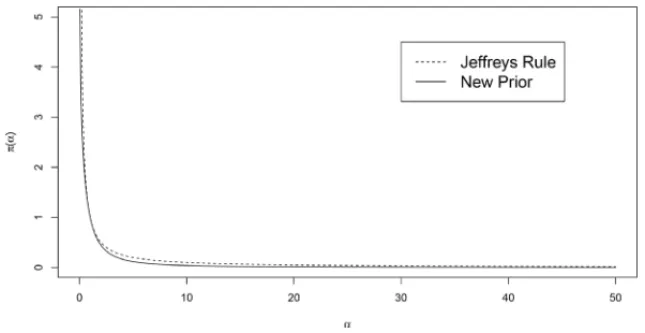
Although different non-informative prior distributions could be considered for the GG distribu-tion as the Jeffreys’ prior or the reference prior [10], such priors involve transcendental funcdistribu-tion inφsuch as digamma and trigamma functions with does not allow us to obtain closed-form esti-mator forφ. A simple non-informative prior distribution representing the lack of information on the parameters can be obtained by using Jeffreys’ rule [10]. As the GG distribution parameters are contained in positive intervals(0,∞), using Jeffreys’ rule the the following prior is obtained
πR(φ, µ, α)∝ 1
φµα. (12)
The joint posterior distribution forφ, µandα, using Jeffreys’ rule is proportional to the product of the likelihood function (2) and the prior distribution (12), resulting in,
pR(φ, µ, α|t)= 1 d1(t)
αn−1 φŴ(φ)nµ
nαφ−1 n
i=1
tiαφ−1
exp
−µα n
i=1
tiα
However, the posterior density (13) is improper, i.e.,
d1(t)=
A αn−1 φŴ(φ)nµ
nαφ−1 n
i=1
tiαφ−1
exp
−µα n
i=1
tiα
dθ = ∞
whereθ=(φ, µ, α)andA= {(0,∞)×(0,∞)×(0,∞)}is the parameter space ofθ.
Proof. Since φŴ(φ)αn−1nµnαφ−1
n i=1t
αφ−1 i
exp
−µαni=1tiα
≥ 0, by Tonelli theorem (see Folland [6]) we have
d1(t)=
A αn−1 φŴ(φ)nµ
nαφ−1 n
i=1
tiαφ−1
exp
−µα n
i=1
tiα dθ = ∞ 0 ∞ 0 ∞ 0
αn−1 φŴ(φ)nµ
nαφ−1 n
i=1
tiαφ−1
exp
−µα n
i=1
tiα
dµdφdα
= ∞ 0 ∞ 0
αn−2 Ŵ(nφ) φŴ(φ)n
n i=1ti
αφ−1 n
i=1tiα
nφ dφdα≥
∞ 0 1 0
c1αn−2φn−2 ⎛
⎝ n
n i=1tiα n
i=1tiα ⎞
⎠ nφ
dφdα
=
∞
0
c1αn−2
γ (n−1,nq(α))
(nq(α))n−1 dα≥ ∞
1
g1
1
αdα= ∞,
where
q(α)=log ⎛
⎝ n
i=1tiα n
n i=1tiα
⎞
⎠>0
andc1andg1are positive constants such that the above inequalities occur. For more details and
proof of the existence of these constants, see Ramos [19].
Since the Jeffreys’ rule prior returned an improper posterior, a modification in this prior was considered. This modified prior is given by
πM(φ, µ, α)∝ 1
φµα12+
α
1+α
· (14)
The present modification had two main objectives. First was to produce a modified prior for π(α)that behave similar toπ(α) ∝ α−1(see Figure 1). Second, was to construct a joint prior distribution that yields a proper posterior distribution.
The joint posterior distribution forφ, µandα, using the prior distribution (14) is proportional to the product of the likelihood function (2) and the prior distribution (14) resulting in,
pM(φ, µ, α|t)= 1 d2(t)
αn−
1
2−α/(1+α)
φŴ(φ)n µ nαφ−1
n
i=1
tiαφ−1
exp
−µα n
i=1
tiα
Figure 1–Plot of the Jeffreys’ Rule and the new Prior considering different values forα.
This joint posterior distribution is proper, i.e.,
d2(t)=
A
αn−12−α/(1+α)
φŴ(φ)n µ nαφ−1
n
i=1
tiαφ−1
exp
−µα n
i=1
tiα
dθ <∞, (16)
whereθ =(φ, µ, α)andA = {(0,∞)×(0,∞)×(0,∞)}is the parameter space ofθ. The
proof of this result is presented in Appendix A at the end of the paper.
The marginal posterior distribution forαandφis obtained by integrating (15) with respect toµ, i.e.,
pM(φ, α|t)= 1 d2(t)
αn−12−α/(1+α)
φŴ(φ)n n
i=1
tiαφ−1
∞
0
µnαφ−1exp
−µα n
i=1
tiα
dµ.
From the result
∞
0
xα−1e−βxd x= Ŵ(α) βα
and considering the transformationv=µα, we have
∞
0
µnαφ−1exp
−µα n
i=1
tiα
dµ= 1 α
∞
0
vnφ−1exp
−v n
i=1
tiα
dv= Ŵ(nφ)
αni=1tiαnφ .
Therefore, the marginal posterior distribution ofαandφis given by
pM(φ, α|t)= 1 d2(t)
αn−
3
2−α/(1+α)
φŴ(φ)n n
i=1
tiαφ−1
Ŵ(nφ) n
The logarithm of the above marginal distribution is given by
log(pM(α, φ|t))=
n−3 2 −
α
(1+α) log(α)+log(Ŵ(nφ))−log(φ)−log(d2)
+(αφ−1) n
i=1
log(ti)−nlog(Ŵ(φ))−nφlog ! n
i=1
tiα "
.
The first-order partial derivatives of log(pM(α, φ|t)), with respect toαandφ, are given, respec-tively, by,
∂log(pM(α, φ|t))
∂α =κ(α)+φ n
i=1
log(ti)−nφ n
i=1tiαlog(ti) n
i=1tiα ,
∂log(pM(α, φ|t))
∂φ =nψ (nφ)+α n
i=1
log(ti)− 1
φ −nψ (φ)−nlog ! n
i=1
tiα "
,
whereκ(α) = #n−32−(1+αα)$1α − α
(1+α)2log(α). The maximum a posteriori estimates ofφ˜
andα˜related to pM(α, φ|t)are obtained by solving
∂log(pM(α, φ|t))
∂α =0 and
∂log(pM(α, φ|t))
∂φ =0.
By solving∂log(pM(α, φ|t)%∂α, we have
˜
φ= κ(α)˜
n i=1tiα˜ #
nni=1tiα˜log(tiα˜)−ni=1tiα˜ni=1log(tiα˜)$·
(17)
By solving∂log(pM(α, φ|t)%∂φand replacingφbyφ˜ we haveα˜ can be obtained finding the minimum of
h(α)=nψ#nφ˜$+α n
i=1
log(ti)− 1
˜
φ−ψ #
˜
φ$−log ! n
i=1
tiα "
(18)
Using one dimensional iterative methods, we obtain the value ofα. Replacing˜ α˜ in equation (17), we haveφ. The preliminary estimate˜ µcan be obtained from
∂log(pM(φ, µ, α|t))
∂µ =(nφ˜α˜−1)− ˜αµ˜ ˜
α n
i=1
tiα˜ =0
and after some algebraic manipulation,
˜ µ= ⎧ ⎪ ⎪ ⎪ ⎪ ⎨ ⎪ ⎪ ⎪ ⎪ ⎩
nα˜φ˜−1
˜
αn i=1tiα˜
1
˜
α
, if nα˜φ >˜ 1
nφ˜
n
i=1tiα˜ 1
˜
α
, if nα˜φ <˜ 1
This approach can be easily used to find good initial valuesφ,˜ µ˜ andα. These results are of˜
great practical interest since it can be used in a Bayesian analysis to construct empirical prior distributions forφ, µandαas well as for initialization of the iterative methods to find the MLEs of the GG distribution parameters.
5 A NUMERICAL ANALYSIS
In this section, a simulation study via Monte Carlo method is performed in order to study the ef-fect of the initial values obtained from (17, 18 and 19) in the MLEs and posterior estimates, considering complete and censored data. In addition, MCMC (Markov Chain Monte Carlo) methods are used to obtain the posterior summaries. The influence of sample sizes on the ac-curacy of the obtained estimates was also investigated. The following procedure was adopted in the study:
1. Set the values ofθ=(φ, µ, α)and n.
2. Generate values of the GG(φ, µ, α)distribution with sizen.
3. Using the values obtained in step (2), calculate the estimates ofφ,ˆ µˆ andαˆusing the MLEs or the Bayesian inference for the parametersφ, µandα.
4. Repeat (2) and (3)N times.
The chosen values for this simulation study are θ =((0.5,0.5,3),(0.4,1.5,5))and n = (50, 100,200). The seed used to generate the random values in the R software is 2013. The com-parison between the methods was made through the calculation of the averages and standard deviations of the N estimates obtained through the MLEs and posterior means. It is expected that the best estimation method has the means of theN estimates closer to the true values ofθ
with smaller standard deviations. It is important to point out that, the results of this simulation study were similar for different values ofθ.
5.1 A classical analysis
In the lack of information on which initial values should be used in the iterative method, we generate random values such thatφ˜ ∼U(0,5),µ˜ ∼U(0,5)andα˜ ∼U(0,5). This procedure is denoted as “Method 1”. On the other hand, from equations (17, 18 and 19), good initial val-ues are easily obtained to be used in iterative methods to get the MLEs considering complete observations. In the presence of censored observations we discuss the possibility of using only the complete observations, in order to obtain good initial valuesφ,˜ µ˜ andα. This procedure is˜ denoted as “Method 2”.
Table 1–Estimates of the means and standard deviations of MLE’s and coverage probabilities with
a nominal 95% confidence level obtained from 50,000 samples using Method 1 for different values ofθandn, using complete observations as well as censored observations (20% censoring).
Complete observations Censored observations
n=50 n=100 n=200 n=50 n=100 n=200
θ
Mean(SD) Mean(SD) Mean(SD) Mean(SD) Mean(SD) Mean(SD)
MLE MLE MLE MLE MLE MLE
φ=0.5 1.940(1.416) 1.806(1.335) 1.788(1.248) 1.105(1.323) 1.026(1.202) 0.981(1.149) µ=0.5 1.816(1.973) 1.692(1.850) 1.646(1.821) 1.112(1.983) 1.033(1.876) 0.997(1.835) α=3 1.827(1.260) 1.821(1.061) 1.742(0.921) 3.565(2.863) 3.254(2.218) 3.091(1.834) φ=0.4 1.094(0.968) 1.050(0.957) 0.983(0.970) 0.667(0.882) 0.659(0.936) 0.535(0.544) µ=1.5 2.318(1.724) 2.386(3.729) 2.352(4.507) 1.842(1.617) 1.872(2.110) 1.608(0.894) α=5 3.548(2.003) 3.539(4.282) 3.526(1.492) 6.266(4.290) 5.686(3.180) 5.379(2.613)
CP CP CP CP CP CP
φ=0.5 97.96% 98.17% 98.52% 70.59% 65.67% 61.67% µ=0.5 98.31% 98.36% 98.62% 79.61% 72.29% 64.35%
α=3 44.64% 39.49% 29.58% 71.05% 67.27% 63.38%
φ=0.4 98.30% 98.80% 98.80% 77.40% 74.00% 75.00% µ=1.5 99.20% 99.00% 98.90% 83.10% 77.50% 77.20%
α=5 63.90% 52.30% 47.80% 79.40% 75.80% 76.60%
Table 2 – Estimates of the means and standard deviations of MLE’s and coverage probabilities
obtained from 50,000 samples using Method 2 for different values ofθ andn, using complete
observations as well as censored observations (20% censoring).
Complete observations Censored observations
n=50 n=100 n=200 n=50 n=100 n=200
θ
Mean(SD) Mean(SD) Mean(SD) Mean(SD) Mean(SD) Mean(SD)
IV IV IV IV IV IV
φ=0.5 0.675(0.211) 0.686(0.141) 0.689(0.092) 0.759 0.793 0.599 0.429 0.532(0.223) µ=0.5 0.572(0.124) 0.571(0.069) 0.570(0.043) 0.713 1.148 0.565 0.399 0.519(0.101) α=3 2.576(0.432) 2.493(0.316) 2.450(0.224) 3.282 1.616 3.296 1.283 3.201(0.895) φ=0.4 0.646 0.157 0.661(0.105) 0.674 0.071 0.752 0.716 0.543(0.312) 0.456(0.157) µ=1.5 1.695 0.170 1.703(0.110) 1.711 0.073 1.876 1.225 1.629(0.333) 1.549(0.131) α=5 3.742 0.564 3.619(0.410) 3.538 0.293 4.204 1.602 4.603(1.299) 4.867(1.012) Mean(SD) Mean(SD) Mean(SD) Mean(SD) Mean(SD) Mean(SD)
MLE MLE MLE MLE MLE MLE
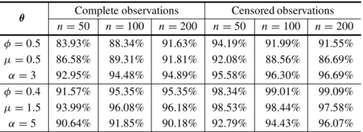
Table 3–95% confidence level obtained from 50,000 samples using Method 2
for different values ofθandn, using complete observations as well as censored
observations (20% censoring).
θ Complete observations Censored observations
n=50 n=100 n=200 n=50 n=100 n=200
φ=0.5 83.93% 88.34% 91.63% 94.19% 91.99% 91.55%
µ=0.5 86.58% 89.31% 91.81% 92.08% 88.56% 86.69%
α=3 92.95% 94.48% 94.89% 95.58% 96.30% 96.69%
φ=0.4 91.57% 95.35% 95.35% 98.34% 99.01% 99.09%
µ=1.5 93.99% 96.08% 96.18% 98.53% 98.44% 97.58%
α=5 90.64% 91.85% 90.18% 92.79% 94.43% 96.07%
We can observe in the results shown in Tables 1 to 3, that the MLEs are strongly affected by the initial values. For example, using method 1, forµ =0.5andn=50, the average obtained from N = 50,000 estimates ofµis equal to 1.816, with standard deviation equals to 1.973. Other problem using such methodology is that the coverage probability tends to decrease even considering large sample sizes.
Using our proposed methodology (method 2) it can be seen that in all cases the method gives good estimates forφ, αandµ. The coverage probabilities of parameters show that, as the sam-ple size increase the intervals tend to 95% as expected. Therefore, we can easily obtain good inferences for the parameters of the GG distribution for both, complete or censored data sets.
5.2 A Bayesian analysis
From the Bayesian approach, we can obtain informative hyperparameter for the gamma prior distribution using the method of moments (11) with mean given byλ=(φ,˜ µ,˜ α), obtained using˜ the equations (17-19). Additional, we have assumed the variance given byσ2
θ =(1,1,1),σ 2 θ =
(φ,˜ µ,˜ α)˜ andσ2
θ = (10,10,10)to verify which of these values produce better results. The
procedure was replicated consideringN=1,000 for different values of the parameters.
The OpenBUGS was used to generate chains of the marginal posterior distributions ofφ, µand αvia MCMC methods. The code is given by
model<-function () { for (i in 1:N) {
x[i] ˜ dggamma(phi,mu,alpha) }
phi ˜ dgamma(phi1,phi2) mu ˜ dgamma(mi1,mi2)
alpha˜ dgamma(alpha1,alpha2)
In the case of censored data, we only have to change dggamma(phi,mu,alpha) in the code above by dggamma(phi,mu,alpha)I(delta[i],). The hyperparametersphi1,phi2,. . . ,alpha2are obtained by our initial values. The main advantage of using the OpenBUGS is due its simplicity, here, the proposal distribution for generating the marginal distributions are defined by the program according to its structure. Therefore we only have to set the data to be fitted. For each simulated sample 8,500 iterations were performed. As “burn-in samples”, we discarded the 1000 initial values. To decrease the autocorrelations bettwen the samples in each chain, the thin considered was 15, obtaining at the end three chains of size 500, these results were used to obtain the posterior summaries forφ, µ andα. The convergence of the Gibbs sampling algorithm was confirmed by the Geweke criterion [7] under a 95% confidence level.
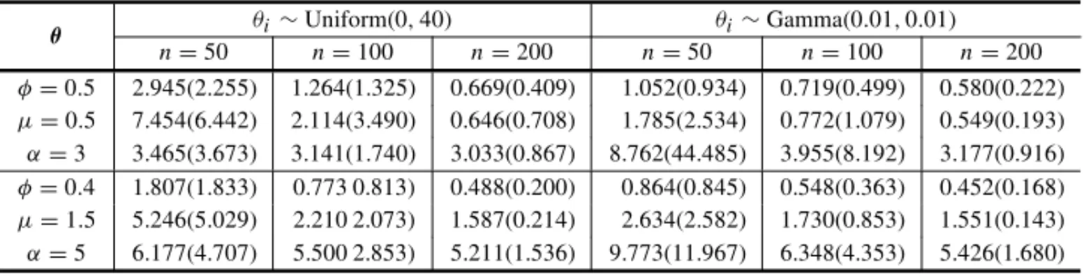
To illustrated the importance of good initial values and informative priors, firstly we considered a simulation study using flat priors, i.e., prior distributions that have large variance, here we assume thatθi ∼Uniforme(0,40),i =1, . . . ,3 orθi ∼Gamma(0.01,0.01). Table 4 displays the means, standard deviations of the posterior means from 1000 samples obtained using the flat priors calculated for different values ofθandn.
Table 4–Means and standard deviations from initial values and posterior means subsequently ob-tained from 1000 simulated samples with different values ofθandn, using the gamma prior
distribu-tion withθi∼Uniform(0,40)andθi∼Gamma(0.01,0.01).
θi∼Uniform(0,40) θi∼Gamma(0.01,0.01)
θ
n=50 n=100 n=200 n=50 n=100 n=200
φ=0.5 2.945(2.255) 1.264(1.325) 0.669(0.409) 1.052(0.934) 0.719(0.499) 0.580(0.222) µ=0.5 7.454(6.442) 2.114(3.490) 0.646(0.708) 1.785(2.534) 0.772(1.079) 0.549(0.193) α=3 3.465(3.673) 3.141(1.740) 3.033(0.867) 8.762(44.485) 3.955(8.192) 3.177(0.916) φ=0.4 1.807(1.833) 0.773 0.813) 0.488(0.200) 0.864(0.845) 0.548(0.363) 0.452(0.168) µ=1.5 5.246(5.029) 2.210 2.073) 1.587(0.214) 2.634(2.582) 1.730(0.853) 1.551(0.143) α=5 6.177(4.707) 5.500 2.853) 5.211(1.536) 9.773(11.967) 6.348(4.353) 5.426(1.680)
From this table, we observe that flat priors with vague information may affect the posterior estimates, specially for small sample sizes, for instance in the case ofn = 50 andα = 3.0 we obtained the mean of the estimates given by 8.762 with standard deviation 44.485 which is undesirable. On the other hand, tables 5-6 display the means, standard deviations and the coverage probabilities of the estimates of 1000 samples obtained using the initial values (IV) and the Bayesian estimates (BE) of the posterior means, calculated for different values ofθ andn,
using complete data.
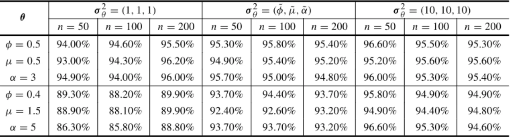
We observed from Tables 5-6 that using the values calculated from equations (17-19) in the method of moments (11) with meanλ=θ˜and with varianceσ2
θ =θ˜to get the hyperparameter
values of the gamma distribution, we obtained very good posterior summaries forφ, µandα, under a Bayesian approach.
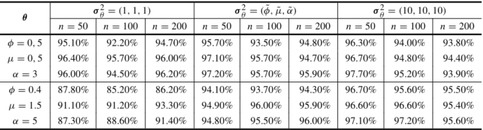
Table 5– Coverage probabilities with a confidence level of 95% of the estimates of posterior means
obtained from 1000 simulated samples of sizen=(50,100,200), with different values ofθ, using the gamma prior distribution withλ=(φ,˜ µ,˜ α),˜ σ2
θ =(1,1,1),σ2θ =(φ,˜ µ,˜ α)˜ andσ2θ =(10,10,10)and
complete observations.
θ σ
2
θ =(1,1,1) σ2θ=(φ,˜ µ,˜ α)˜ σ2θ=(10,10,10) n=50 n=100 n=200 n=50 n=100 n=200 n=50 n=100 n=200 φ=0.5 94.00% 94.60% 95.50% 95.30% 95.80% 95.40% 96.60% 95.50% 95.30% µ=0.5 93.00% 94.30% 96.20% 94.90% 95.40% 95.20% 95.20% 95.60% 95.60% α=3 94.90% 94.00% 96.00% 95.70% 95.00% 94.80% 96.00% 95.30% 95.40% φ=0.4 89.30% 88.20% 89.90% 93.70% 94.40% 93.70% 95.80% 94.90% 94.90% µ=1.5 88.90% 88.10% 89.90% 92.40% 92.60% 93.20% 94.90% 94.40% 94.80% α=5 86.30% 85.80% 88.80% 93.70% 93.70% 93.20% 96.60% 95.30% 94.60%
Table 6–Means and standard deviations from initial values and posterior means subsequently obtained
from 1000 simulated samples with different values ofθandn, using the gamma prior distribution with
λ=(φ,˜ µ,˜ α),˜ σ2
θ =(1,1,1),σ2θ =(φ,˜ µ,˜ α)˜ andσ2θ =(10,10,10)assuming complete observations.
θ σ
2
θ =(1,1,1) σ2θ =(φ,˜ µ,˜ α)˜ σ2θ =(10,10,10) n=50 Mean(SD) Mean(SD) Mean(SD) Mean(SD) Mean(SD) Mean(SD)
IV BE IV BE IV BE
φ=0.5 0.674(0.184) 0.741(0.300) 0.676(0.193) 0.729(0.327) 0.667(0.190) 0.893(0.603) µ=0.5 0.572(0.097) 0.624(0.166) 0.572(0.101) 0.623(0.177) 0.568(0.100) 0.879(0.611) α=3 2.572(0.439) 2.767(0.634) 2.567(0.442) 2.983(0.858) 2.592(0.432) 3.423(1.466) φ=0.4 0.629(0.135) 0.641(0.212) 0.629(0.137) 0.636(0.264) 0.625(0.128) 0.706(0.416) µ=1.5 1.683(0.142) 1.701(0.205) 1.684(0.145) 1.712(0.256) 1.678(0.138) 1.837(0.481) α=5 3.772(0.551) 4.004(0.697) 3.767(0.554) 4.454(1.082) 3.779(0.545) 4.981(1.630) n=100 Mean(SD) Mean(SD) Mean(SD) Mean(SD) Mean(SD) Mean(SD)
IV BE IV BE IV PD
φ=0.5 0.684(0.126) 0.678(0.240) 0.685(0.129) 0.661(0.258) 0.679(0.125) 0.690(0.372) µ=0.5 0.569(0.060) 0.583(0.117) 0.569(0.061) 0.578(0.124) 0.568(0.062) 0.635(0.290) α=3 2.489(0.304) 2.805(0.568) 2.495(0.311) 2.981(0.747) 2.502(0.307) 3.238(1.086) φ=0.4 0.636(0.099) 0.590(0.166) 0.635(0.095) 0.555(0.204) 0.635(0.098) 0.552(0.277) µ=1.5 1.680(0.102) 1.652(0.155) 1.680(0.098) 1.634(0.186) 1.679(0.100) 1.646(0.278) α=5 3.698(0.422) 4.143(0.650) 3.701(0.424) 4.650(1.052) 3.707(0.417) 5.112(1.475) n=200 Mean(SD) Mean(SD) Mean(SD) Mean(SD) Mean(SD) Mean(SD)
IV BE IV BE IV BE
random samples under the same conditions described in the beginning of this section. Tables 7-8 display the means, standard deviations and the coverage probabilities of the estimates of 1000 samples obtained using the initial values and the Bayes estimates of the posterior means, calculated for different values ofθandn, using censored observations (20% censoring).
Table 7– Coverage probabilities with a confidence level of 95% of the estimates of posterior means
obtained from 1000 simulated samples of sizen= (50,100,200), with different values ofθ, using the
gamma prior distribution withλ=(φ,˜ µ,˜ α),˜ σ2
θ=(1,1,1),σ2θ =(φ,˜ µ,˜ α)˜ andσ2θ =(10,10,10)and
censored observations (20% of censoring).
θ σ
2
θ=(1,1,1) σ2θ=(φ,˜ µ,˜ α)˜ σ2θ=(10,10,10) n=50 n=100 n=200 n=50 n=100 n=200 n=50 n=100 n=200 φ=0,5 95.10% 92.20% 94.70% 95.70% 93.50% 94.80% 96.30% 94.00% 93.80% µ=0,5 96.40% 95.70% 96.00% 97.10% 95.70% 94.70% 96.70% 94.80% 94.40% α=3 96.00% 94.50% 96.20% 97.20% 95.70% 95.90% 97.70% 95.20% 93.90% φ=0.4 87.80% 85.20% 86.20% 94.10% 93.70% 94.30% 96.70% 95.60% 95.50% µ=1.5 91.10% 91.20% 93.30% 94.90% 96.00% 95.90% 96.60% 96.60% 95.40% α=5 87.30% 88.60% 91.40% 94.80% 95.50% 96.00% 97.10% 97.20% 95.60%
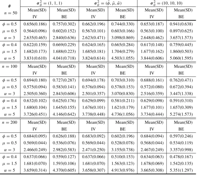
From Tables 7-8 that using the values calculated from equations (17-19) in the method of mo-ments (11) with mean λ = θ˜ and with varianceσ2
θ =θ˜are usefull to get the hyperparameter
values of the gamma distribution under censored data allowing us to obtain good posterior sum-maries forφ, µandα, under a Bayesian approach.
6 REAL DATA APPLICATIONS
In this section, the proposed methodology is applied using two data sets from the literature. The GG distribution is assumed to analyze these data sets and the obtained results are compared with other models such as the Weibull, Gamma and Lognormal distributions, using the Akaike information criterion (AI C = −2l(αˆ;x)+2k), corrected Akaike information criterion (AI Cc =
AI C+(2k(k+1))/(n−k−1)) and the Bayesian information criterion (B I C = −2l(αˆ;x)+
klog(n)), wherekis the number of parameters to be fitted andαˆis the estimate ofα. In all cases,
Bayesian approach is used to obtain the estimates of the parameters for the different distributions. Addionaly, we assume gamma priors with hyperparameters values equal to 0.1 for the parameters of the Weibull, Gamma and Lognormal distributions. For each case, 30,000 Gibbs samples were simulated using MCMC methods taking every 15t hgenerated sample obtaining a final sample of size 2,000 to be used to get the posterior summaries.
6.1 Remission times of patients with cancer
Table 8–Means and standard deviations from initial values and posterior means subsequently
ob-tained from 1000 simulated samples with different values ofθandn, using the gamma prior
distribu-tion withλ=(φ,˜ µ,˜ α),˜ σ2
θ =(1,1,1),σ2θ =(φ,˜ µ,˜ α)˜ andσ2θ =(10,10,10)assuming censored
data (20% censoring).
θ σ
2
θ =(1,1,1) σ2θ =(φ,˜ µ,˜ α)˜ σ2θ =(10,10,10) n=50 Mean(SD) Mean(SD) Mean(SD) Mean(SD) Mean(SD) Mean(SD)
IV BE IV BE IV BE
φ=0.5 0.656(0.186) 0.757(0.302) 0.662(0.196) 0.744(0.330) 0.653(0.187) 0.941(0.638) µ=0.5 0.564(0.096) 0.602(0.152) 0.567(0.101) 0.603(0.166) 0.563(0.100) 0.897(0.625) α=3 2.635(0.465) 2.840(0.636) 2.623(0.471) 3.098(0.869) 2.648(0.462) 3.657(1.573) φ=0.4 0.622(0.159) 0.669(0.229) 0.624(0.165) 0.665(0.284) 0.617(0.148) 0.759(0.445) µ=1.5 1.682(0.173) 1.688(0.223) 1.685(0.181) 1.704(0.279) 1.677(0.162) 1.860(0.503) α=5 3.831(0.610) 4.041(0.718) 3.824(0.614) 4.503(1.055) 3.844(0.606) 5.060(1.595) n=100 Mean(SD) Mean(SD) Mean(SD) Mean(SD) Mean(SD) Mean(SD)
IV BE IV BE IV BE
φ=0.5 0.694(0.180) 0.727(0.287) 0.694(0.178) 0.703(0.310) 0.688(0.161) 0.762(0.471) µ=0.5 0.575(0.094) 0.583(0.141) 0.576(0.094) 0.578(0.153) 0.572(0.080) 0.672(0.394) α=3 2.505(0.360) 2.843(0.606) 2.501(0.357) 3.070(0.830) 2.516(0.359) 3.447(1.338) φ=0.4 0.632(0.102) 0.625(0.176) 0.629(0.099) 0.581(0.211) 0.629(0.098) 0.591(0.310) µ=1.5 1.680(0.104) 1.645(0.155) 1.676(0.101) 1.621(0.179) 1.677(0.101) 1.657(0.309) α=5 3.726(0.451) 4.146(0.642) 3.738(0.448) 4.736(1.056) 3.734(0.444) 5.274(1.573) n=200 Mean(SD) Mean(SD) Mean(SD) Mean(SD) Mean(SD) Mean(SD)
IV BE IV BE IV BE
φ=0.5 0.684(0.095) 0.626(0.188) 0.683(0.092) 0.602(0.196) 0.684(0.094) 0.597(0.246) µ=0.5 0.569(0.044) 0.536(0.076) 0.569(0.044) 0.528(0.078) 0.568(0.044) 0.534(0.119) α=3 2.466(0.249) 2.982(0.583) 2.471(0.250) 3.155(0.738) 2.467(0.249) 3.357(0.998) φ=0.4 0.637(0.066) 0.559(0.127) 0.637(0.066) 0.510(0.153) 0.634(0.063) 0.478(0.167) µ=1.5 1.681(0.070) 1.593(0.106) 1.681(0.070) 1.563(0.123) 1.678(0.069) 1.542(0.135) α=5 3.659(0.314) 4.370(0.605) 3.658(0.307) 4.913(0.976) 3.665(0.308) 5.351(1.297)
From equations (17-19), we haveφ˜ = 0.5665,µ˜ = 0.2629 and α˜ = 1.4669. Using (11) and assuming as meanλ =θ˜ and varianceσ2
θ =θ˜, we obtain the priorsφ ∼Gamma(0.5665,1),
µ ∼Gamma(0.2629,1)andα ∼Gamma(1.4669,1). The posterior summaries obtained from MCMC methods are given in Table 10.
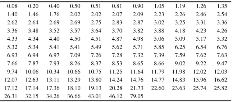
Figure 2 shows the survival function fitted by the different probability distributions and the em-pirical survival function. Table 10 presents the results of the AIC, AICc and BIC criteria for the different probability distributions, considering the blader cancer data introduced in Table 8.
Table 9–Remission times (in months) of a random sample of 128 bladder cancer patients.
0.08 0.20 0.40 0.50 0.51 0.81 0.90 1.05 1.19 1.26 1.35
1.40 1.46 1.76 2.02 2.02 2.07 2.09 2.23 2.26 2.46 2.54
2.62 2.64 2.69 2.69 2.75 2.83 2.87 3.02 3.25 3.31 3.36
3.36 3.48 3.52 3.57 3.64 3.70 3.82 3.88 4.18 4.23 4.26
4.33 4.34 4.40 4.50 4.51 4.87 4.98 5.06 5.09 5.17 5.32
5.32 5.34 5.41 5.41 5.49 5.62 5.71 5.85 6.25 6.54 6.76
6.93 6.94 6.97 7.09 7.26 7.28 7.32 7.39 7.59 7.62 7.63
7.66 7.87 7.93 8.26 8.37 8.53 8.65 8.66 9.02 9.22 9.47
9.74 10.06 10.34 10.66 10.75 11.25 11.64 11.79 11.98 12.02 12.03 12.07 12.63 13.11 13.29 13.80 14.24 14.76 14.77 14.83 15.96 16.62 17.12 17.14 17.36 18.10 19.13 20.28 21.73 22.60 23.63 25.74 25.82 26.31 32.15 34.26 36.66 43.01 46.12 79.05
Table 10–Posterior medians, standard deviations and 95% credibility intervals forφ , µandα.
θ Median SD C I95%(θ )
φ 2.5775 0.7485 (1.3444; 4.2175)
µ 0.5712 0.7215 (0.1575; 2.5821)
α 0.6300 0.1110 (0.4789; 0.9183)
Figure 2–Survival function fitted by the empirical and by different p.d.f considering the bladder cancer data set and the hazard function fitted by a GG distribution.
6.2 Data from an industrial experiment
Table 11–Results of AIC, AICc and BIC criteria for different probability
distributions considering the bladder cancer data set introduced in Table 8.
Criteria G. Gamma Weibull Gamma Lognormal
AIC 828.05 832.15 830.71 834.17
AICc 828.24 832.25 830.81 834.27
BIC 836.61 837.86 836.42 839.88
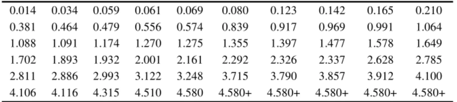
Table 12–Data set of cycles to failure for a group of 60 electrical appliances in a life test (+ indicates the presence of censorship).
0.014 0.034 0.059 0.061 0.069 0.080 0.123 0.142 0.165 0.210
0.381 0.464 0.479 0.556 0.574 0.839 0.917 0.969 0.991 1.064
1.088 1.091 1.174 1.270 1.275 1.355 1.397 1.477 1.578 1.649
1.702 1.893 1.932 2.001 2.161 2.292 2.326 2.337 2.628 2.785
2.811 2.886 2.993 3.122 3.248 3.715 3.790 3.857 3.912 4.100
4.106 4.116 4.315 4.510 4.580 4.580+ 4.580+ 4.580+ 4.580+ 4.580+
From equations (17-19), we haveφ˜ = 0.5090,µ˜ = 0.2746 and α˜ = 1.7725. Using (11) and assuming as meanλ = θ˜and variance σ2
θ = θ˜, we elicit the priorsφ ∼ Gamma(0.5090,1),
µ ∼Gamma(0.2746,1)andα ∼Gamma(1.7725,1). The posterior summaries obtained from MCMC methods are given in Table 13.
Table 13–Posterior medians, standard deviations
and 95% credibility intervals forφ , µandα.
θ Median SD C I95%(θ )
φ 0.2689 0.1856 (0.1097; 0.8193)
µ 0.1988 0.0632 (0.1538; 0.3685)
α 2.5850 1.3094 (1.0629; 5.6785)
Figure 3 shows the survival function fitted by probability distributions and the empirical survival function. Table 14 presents the results of the AIC, AICc and BIC criteria for different probability distributions, considering the industrial failure data set introduced in Table 12.
Table 14– Results of DIC criteria, AIC and BIC for different probability distributions considering the data of cycles to failure introduced in Table 11.
Criteria G. Gamma Weibull Gamma Lognormal
AIC 199.19 202.11 201.80 216.55
AICc 199.62 202.32 202.01 216.76
Figure 3–Survival function fitted by the empirical and different p.d.f considering the data set related to
the industrial data set and the hazard function fitted by a GG distribution.
Based on the AIC and AICc criteria, we concluded from Table 14 that the GG distribution has the best fit for the industrial data. Additionally, the GG distribution is the only one between probability distributions assumed that allows bathtub shape hazard. This is an important point for the use of the GG distribution in applications.
7 CONCLUDING REMARKS
The generalized gamma distribution has played an important role as lifetime data, providing great flexibility of fit. In this paper, we showed that under the classical and Bayesian approaches, the parameter estimates usually do not exhibit stable performance in which can lead, in many cases, to different results.
This problem is overcome by proposing some empirical exploration methods aiming to obtain good initial values to be used in iterative procedures to find MLEs for the parameters of the GG distribution. These values were also used to elicit empirical prior distributions (use of empirical Bayesian methods). These results are of great practical interest since the GG distribution can be easily used as appropriated model in different applications.
ACKNOWLEDGEMENTS
REFERENCES
[1] AHSANULLAHM, MASWADAHM & ALIMS. 2013. Kernel inference on the generalized gamma distribution based on generalized order statistics.Journal of Statistical Theory and Applications, 12(2): 152–172.
[2] MOALAAF, RAMOSLP & ACHCARAJ. 2013. Bayesian inference for two-parameter gamma distri-bution assuming different noninformative priors.Revista Colombiana de Estad´ıstica,36(2): 319–336.
[3] ASHKARF, BOBEE´ B, LEROUXD & MORISETTED. 1988. The generalized method of moments as applied to the generalized gamma distribution.Stochastic Hydrology and Hydraulics,2(3): 161–174.
[4] COXC, CHUH, SCHNEIDERMF & MUNOZ˜ A. 2007. Parametric survival analysis and taxonomy of hazard functions for the generalized gamma distribution.Statistics in Medicine,26(23): 4352–4374.
[5] DICICCIOT. 1987. Approximate inference for the generalized gamma distribution.Technometrics, 29(1): 33–40.
[6] FOLLANDGB. 2013.Real analysis: modern techniques and their applications. John Wiley & Sons.
[7] GEWEKEJET AL. 1991.Evaluating the accuracy of sampling-based approaches to the calculation of posterior moments, vol. 196. Federal Reserve Bank of Minneapolis, Research Department Min-neapolis, MN, USA.
[8] HAGERHW & BAINLJ. 1970. Inferential procedures for the generalized gamma distribution. Jour-nal of the American Statistical Association,65(332): 1601–1609.
[9] HUANGP-H & HWANG T-Y. 2006. On new moment estimation of parameters of the generalized gamma distribution using it’s characterization.Taiwanese Journal of Mathematics,10: 1083–1093.
[10] KASSRE & WASSERMANL. 1996. The selection of prior distributions by formal rules.Journal of the American Statistical Association,91(435): 1343–1370.
[11] LAWLESSJF. 2011.Statistical models and methods for lifetime data, vol. 362. John Wiley & Sons.
[12] LEE ET & WANGJ. 2003.Statistical methods for survival data analysis, vol. 476. John Wiley & Sons.
[13] MARTINEZEZ, ACHCARJA,DEOLIVEIRAPERESMV &DEQUEIROZJAM. 2016. A brief note on the simulation of survival data with a desired percentage of right-censored datas.Journal of Data Science,14(4): 701–712.
[14] PARRVB & WEBSTERJ. 1965. A method for discriminating between failure density functions used in reliability predictions.Technometrics,7(1): 1–10.
[15] PASCOAMA, ORTEGAEM & CORDEIROGM. 2011. The kumaraswamy generalized gamma dis-tribution with application in survival analysis.Statistical Methodology,8(5): 411–433.
[16] PHAMT & ALMHANAJ. 1995. The generalized gamma distribution: its hazard rate and stress-strength model.IEEE Transactions on Reliability,44(3): 392–397.
[17] PRENTICERL. 1974. A log gamma model and its maximum likelihood estimation.Biometrika,61(3): 539–544.
[19] RAMOSPL. 2014. Aspectos computacionais para inferˆencia na distribuic¸ ˜ao gama generalizada. Dissertac¸˜ao de Mestrado, 165 p.
[20] RAMOSPL, ACHCARJA & RAMOSE. 2014. M´etodo eficiente para calcular os estimadores de m´axima verossimilhanca da distribuic¸ ˜ao gama generalizada.Rev. Bras. Biom.,32(2): 267–281.
[21] RAMOS PL, LOUZADA F & RAMOS E. 2016. An efficient, closed-form map estimator for nakagami-m fading parameter.IEEE Communications Letters,20(11): 2328–2331.
[22] SHINJW, CHANGJ-H & KIMNS. 2005. Statistical modeling of speech signals based on generalized gamma distribution.IEEE Signal Processing Letters,12(3): 258–261.
[23] STACYEW. 1962. A generalization of the gamma distribution.The Annals of Mathematical Statistics, 1187–1192.
[24] STACY EW & MIHRAMGA. 1965. Parameter estimation for a generalized gamma distribution.
Technometrics,7(3): 349–358.
[25] WINGODR. 1987. Computing maximum-likelihood parameter estimates of the generalized gamma distribution by numerical root isolation.IEEE Transactions on Reliability,36(5): 586–590.
APPENDIX A
Proof. Since α n−1
2−α/(1+α)
φŴ(φ)n µ
nαφ−1n i=1t
αφ−1
i exp
−µαni=1tiα ≥ 0 by Tonelli theorem [6] we have
d2=
∞ 0 ∞ 0 ∞ 0
αn−
1
2−α/(1+α)
φŴ(φ)n µ nαφ−1
n
i=1
tiαφ−1
exp
−µα n
i=1
tiα
dµdφdα=
= ∞ 0 ∞ 0
αn−
3 2−
α (1+α)
φŴ(φ)n n
i=1
tiαφ−1
Ŵ(nφ) n
i=1tiα
nφdφdα=s1+s2+s3+s4,
where
s1= 1 0 1 0
αn−
3 2−
α (1+α)
φŴ(φ)n n
i=1
tiαφ−1
Ŵ(nφ) n
i=1tiα
nφdφdα
<
1
0
c′1αn−
3 2−
α
(1+α)γ (n−1,nq(α))
(nq(α))n−1 dα < 1
0
g1′αn−
3
2dα <∞.
s2=
∞ 1 1 0
αn−
3 2−
α (1+α)
φŴ(φ)n n
i=1
tiαφ−1
Ŵ(nφ) n
i=1tiα
nφdφdα
< ∞
1
c′1αn−
3 2−
α
(1+α)γ (n−1,nq(α))
(nq(α))n−1 dα <
∞
1
g2′α−
3
s3= 1
0
∞
1
αn−
3 2−
α (1+α)
φŴ(φ)n n
i=1
tiαφ−1
Ŵ(nφ)
n
i=1tiα
nφdφdα,
<
1
0
c2an−
3 2−
α
1+αŴ( n−1
2 ,np(α))
(np(α))n−21
dα <
1
0
g3′α−
1
2dα <∞.
s4=
∞
1
∞
1
αn−
3 2−
α (1+α)
φŴ(φ)n n
i=1
tiαφ−1
Ŵ(nφ) n
i=1tiα
nφdφdα
< ∞
1
c2an−
3 2−1+ααŴ(
n−1
2 ,np(α))
(np(α))n−21
dα < ∞
1
g4′α−
3
2dα <∞.
wherec′1,c′2,g′1,g′2,g′3andg′4are positive constants such that the above inequalities occur. For more details and proof of the existence of these constants, see Ramos [19]. Therefore, we have: