B-WIM systems application on reinforced concrete
bridge structural assessment and highway traic
characterization
Aplicação de sistemas B-WIM para avaliação
estrutural e caracterização do tráfego em uma ponte
de concreto armado
a Civil Engineering Department, Federal University of Mato Grosso;
b Programa de Pós Graduação em Engenharia Civil, Universidade Federal de Santa Catarina, Florianópolis, Santa Catarina, Brasil.
Received: 07 Dec 2016 • Accepted: 20 Mar 2017 • Available Online: 11 Dec 2017
P. JUNGES a
R. C. A. PINTO b
L. F. FADEL MIGUEL b
Abstract
Resumo
The vehicles that travel on Brazilian highways have changed a lot in the last decades, with an increase in the trafic load and in the amount of
trucks. This fact is not exclusive to our country, so much that in order to assess the structural safety of bridges, there was a great development in
bridge weigh-in-motion systems (WIM) the last decade, especially in developed countries. Moses, in 1979, was the irst one to introduce the
B-WIM concept. This work presents the results of a B-B-WIM system applied on a bridge over the Lambari river, located at BR 153 in Uruaçu (Goiás).
The weigh-in-motion technique used is based on Moses' Algorithm and uses inluence lines obtained direct from trafic. Trafic characterization of that particular highway, as well as the effects introduced in the bridge structure and the experimental dynamic ampliication factor are also dis -cussed. At the end it is concluded that the system used is capable of detecting, with good precision, the axle spacing and the gross vehicle weight shows errors inferior to 3% when compared with the gross weight acquired with static scale.
Keywords: B-WIM, monitoring, trafic characteristics, bridges, safety.
Os veículos que trafegam nas rodovias brasileiras mudaram muito nas últimas décadas, ocorrendo um aumento na capacidade de carga e na quantidade de caminhões. Esse fato não é exclusivo do nosso país, tanto que na última década houve um grande desenvolvimento dos sistemas de pesagem em movimento em pontes (bridge weigh-in-motion, B-WIM), especialmente nos países desenvolvidos, para avaliação da segurança estrutural de pontes. Moses em 1979 foi o primeiro a introduzir o conceito de B-WIM e o algoritmo por ele desenvolvido continua sendo o mais popular nos sistemas comerciais. No presente estudo são mostrados os resultados da utilização de um sistema B-WIM no monitoramento de uma ponte sobre o rio Lambari, na BR 153, no município de Uruaçu (Goiás). A técnica de pesagem em movimento empregada é baseada no
algoritmo de Moses e utiliza linhas de inluência obtidas diretamente do tráfego. A caracterização do tráfego atuante nessa rodovia, bem como os esforços introduzidos na estrutura da ponte e um coeiciente de impacto obtido de forma experimental são também discutidos. Ao inal conclui-se
que o sistema empregado é capaz de detectar com boa precisão o espaçamento entre os eixos e o peso bruto total dos veículos apresenta erros inferiores a 3% quando comparados com os pesos obtidos em balança estática.
1. Introduction
The live load model used in Brazil has not changed much in the last forty years. Since the NB-6 from 1960 [1], the live load in bridges consists of a standard vehicle with six wheels distributed on three equally spaced axles of 1.5 m. On the other hand, the vehicles that travel on the Brazilian Highways have changed a lot in the last decades, with an increase in the load capacity and in the amount of trucks. Moreover, new classes of vehicles emerged, being common nowadays the presence of trucks up to nine axles and 30 meters long.
Therefore, the load from the trafic should be better assessed to ensure bridge safety. According to [2], these changes in the trafic
need to be regularly taken into account by means of code
calibra-tion. B-WIM systems, which allow the effective estimation of trafic
over the bridge, have had a great development in recent years [3], both in terms of safety assessment of existing structures and on the determination of design loads.
The B-WIM concept was introduced by Moses [4] in the late 70s. An
algorithm with his name uses the inluence line (IL) concept in order to
acquire the weight of the vehicles that travel over bridges with girders. In the 80s, Peters ([5] and [6]) developed weigh-in-motion sys-tems for use on bridges (AXWAY) and culverts (CULWAY), having reached good results for gross vehicle weight estimation (GVW), but inaccurate results for weight of close axles.
In the 90s, two B-WIM systems emerged at the same time in Slo-venia and Ireland [7], both result of the COST 323 [8] and WAVE [9] projects. The DuWIM system was developed by researchers of Trinity College Dublin and University College Dublin. It uses point-to-point manual graphical method to acquire the bridge IL from the passage of a calibration vehicle over the bridge. The SiWIM sys-tem, developed by the Slovenian Institute of Civil Engineering and Construction (ZAG) team, uses an optimization algorithm after the vehicle weight was determined by Moses’ algorithm in order to im-prove the results. In addition, the SiWIM system does not use axle
detection sensors over the bridge. Both DuWIM and SiWIM were also developed to orthotropic bridges applications.
In the 2000s, Yamada and Ojio [10] developed a B-WIM system in which the support stiffeners of a steel bridge are instrumented to measure the vertical strains. However, the method is not very accurate since, according to the authors, only one element is the instrumented.
In all these aforementioned methods, the axles weight identiication
is nothing more than an optimization problem [11]. In this sense, authors like Jiang et al [12], Au et al [13], Law et al [14], Deng and Cai [15], Pan and Yu [16] and Kim et al [17] sought to employ dif-ferent optimization techniques to solve the problem, from the use
of genetic algorithms to artiicial neural networks.
Besides these systems in time domain, several authors proposed methods that use the bridge dynamic response ([18], [19], [20], [21] e [22]). Nevertheless, these methods are still quite complex
and dificult to implement.
In 2005, Karoumi, Wiberg and Liljencrantz [23] extended the B-WIM utilization to railway bridge monitoring. The developed system uses strain transducers placed at different points in order to detect the axles and to calculate the velocity. In Brazil, Carvalho Neto e Veloso
[24] developed a similar system to characterize the railroad trafic.
Despite all the progress, Moses’ algorithm continues to be the ideal choice in the implementation of B-WIM systems due its simplicity and good precision, provided that certain requirements are met
[11]. In this way, in order to assess the eficiency of this system
on the bridges of the Brazilian road network, a bridge at BR 153 highway has been monitored during 42 days. From this monitoring,
information was obtained about the trafic and structure behavior in
terms of IL and internal forces distribution.
2. Bridge weigh-in-motion systems (B-WIM)
Broadly used in developed countries for bridge structural safety as-sessment, B-WIM techniques are already applied in some of these
Figure 1
countries to determine the design live load for bridges. According
to Žnidarič e Žnidarič [25], on B-WIM application, the vehicle stay
in contact with the bridge for a long time period, which makes pos-sible to acquire a large amount of measurements and therefore, smooth the dynamic effects. Besides, the main advantage of a B-WIM system is that it is portable and does not interfere with the
trafic during its installation [2].
B-WIM concepts were irst introduced by Moses [4] in 1979, using
the principle that a live load along the bridge introduce stresses proportional to the product of the IL ordinate with the load magni-tude. The weight of the trucks that travel over a bridge is obtained by a function that minimizes the error between the measured stresses and the theoretical ones.
Thus, a truck traveling with a constant velocity produces a re-sponse that varies over time in equally intervals (k). Observing Figure 1 and considering the superposition principle, the theoretical maximum bending moment, in a k instant, is given by Equation (1).
(1)
where MSTk = theoretical bending moment; N = number of vehicle axles; Pi = weight of the ith vehicle axle; I
i
k = IL ordinate for the ith
axle for k scan.
Moses has used the fact that the stress in each girder is related with bending moment by the relationship indicated in Equation (2) and has acquired the active bending moment in the bridge, in an
instant k, as deined by Equation (3), considering that all girders
have the same properties.
(2)
(3)
where E = modulus of elasticity of the bridge material; Wj = elastic section module for the jth girder; M
SE
k = experimental bending mo-ment in a time instant; m = number of girders; εjk = strain of the jth
girder in a time instant.
Dynamic effects of the truck-pavement-structure system are in-cluded in the value of the experimental bending moment. As the measured response is acquired during the whole passage of the vehicle over the bridge, these dynamic effects can be smoothed out by an error function that minimizes the sum of the squares differences between the experimental and theoretical bending mo-ments, as shown in Equation (4). This minimization process allows to obtain loads closer to the real static values.
(4)
where φ = error function; k = scan number; K = total number of scans.
The minimization process of Equation (4) in relation to the jth axles
results in Equation (5). This equation can be rewritten in a matrix
form, as deined by Equation (6), as a function of the inluence
lines matrix [F] and the vector that relates the measured bending moments and the IL ordinates {M}.
(5)
(6)
(7)
(8)
Figure 2
where T = total number of time intervals used; {P} = vector of axles weight; [F] = inluence lines matrix for bending moment; {M} vector that relates the measured bending moments and the IL ordinates.
Each element of vector {P}, deined by Equation (6), represents the
weight of one of the axles of the vehicle. The GVW is given by the sum of the elements of this vector.
The eficiency of Moses’ algorithm here presented is affected main -ly by the dynamic effect of vehicles in movement, by the transverse
position of the vehicles and the inal equation system [11]. The dy -namic effect of vehicles is directly related to the pavement rough-ness and bridge entrance conditions. The greater the dynamic ef-fects, the lower will be the accuracy of the system, because greater will be the difference between measured and predict response us-ing the static IL. Moreover, the algorithm does not take into account the number of lanes and hence does not account for the transverse
load distribution, which could lead to signiicant errors. Finally, the inal equation system can be ill conditioned in cases where noise in the measured signal is signiicant.
2.1 Calibração do sistema
In his study, Moses has used a theoretical IL in order to acquire trucks weights. However, according to Žnidarič and Baumgart-ner [26], the actual IL of the structure differs from the theoretical one; it is between the idealized conditions of simple supported and
completely ixed support (Figure 2). Several authors have demon -strated the importance of using an IL that better describes the real structural conditions, as Žnidarič and Baumgartner [26], Mc-Nulty [27], González and O’Brien [28], McMc-Nulty and OBrien [29], Quilligan [30], Obrien, Quilligan and Karoumi [31], Junges, Pinto and Fadel Miguel [32], Ieng [33], Heinen, Pinto and Junges [34]. According to Obrien, Quilligan and Karoumi [31], although the IL can be easily obtained from the theoretical or numerical analysis of the struc-ture, the results usually do not meet the ones measured on the bridge, being interesting to acquire the IL directly from the measured stresses coming from the passage of a vehicle with known weight. These au-thors have developed a mathematical method to calculate the IL directly from monitoring data. In the proposed method, there is no need to know the exactly position in which the applied load starts the bending of the bridge. Thus, uncertainty around the real support conditions and the small strain usually induced near the supports are avoided.
Using a vehicle with known axle weights, this method consists to minimize Equation (4) in respect to the Rth IL ordinate, resulting in
the Equation (9) which can be rewritten in matrix form as shown in Equation (10).
(9)
(10)
where [W] = sparse and symmetric matrix dependent of axle weights; {I} = vector containing the IL ordinates; {MP} vector de-pendent of measured bending moments and axle weights. The IL ordinates are obtained by according to Equation (11).
(11)
This procedure was validated on two reinforced concrete bridges located in Sweden [31], reaching excellent correlation between the measured response and the predicted one with the acquired IL. Nevertheless, this method may require a high computational cost, since it is necessary to invert a matrix that, for a three-axle truck and acquisition frequency of 1024 Hz, may be in the order of 1500 and 2000.
The B-WIM system used in the present study, developed initially
by Žnidarič, Žnidarič e Terčelj [35], uses ILs obtained by means
of the procedure proposed by [31] from the passage of trucks with known weights over the bridge. The IL calibration follows the indication of the COST 323 [8] report and the recommendations about weigh-in-motion published by ISWIM [36] to ensure a good quality in the results.
Based on the COST 323 [8] report, the calibration process of B-WIM systems, i.e., obtaining the actual bridge IL, consists of pass-ing vehicles with known weights over the system several times. The greater the number of passages, the greater the accuracy of the system. These passages should be done with at least two ve-hicle classes (rigid and semi-trailer) at two velocity levels.
2.2 Axle detection sensors
In order to obtain velocity information, axle spacing and vehicle class that travel in the highway, strain transducers, called free-of-axle detector (FAD) sensors, are placed on the bottom of the bridge superstructure instrumented with B-WIM systems [37]. The FAD sensors are installed at a certain distance along the bridge length so that it is possible to acquire similar signals spaced by a time interval, as can be seen in Figure 3 for the passage of a 5-axle truck. From these signals, the vehicle velocity is calculated by an optimization process that results on the time interval which
minimizes the difference between sensors readings [7], as deined
by Equation (12).
(12)
where ξ = objective function; Δt = time for the truck to pass be -tween two instrumented sections; TT = total time for the truck to
Figure 3
pass the two instrumented sections; ε1 e ε2 = strain measured in section 1 e 2, respectively.
Figure 4 shows an example of the behavior of objective function (ξ)
with time interval (Δt) varying between 0 and 1 s. From this igure,
it is clear that a minimum global value for the time interval exists. Knowing the distance between sensors and using the time interval obtained by this optimization process, it is possible to acquire the vehicle velocity.
2.3 Dynamic ampliication factor
The dynamic ampliication factor, or impact coeficient, is calcu -lated by the relationship between measured and static response, according to Equation (13).
(13)
where DAF = dynamic ampliication factor; εSE,max = measured
re-sponse; εST,max= static response.
The static response can be obtained by the signal reconstruction, from
the IL and axle weights, or by means of low-pass ilters in the measured
signal. The latter leading to better results (ARCHES D10 [38]).
Low-pass ilters eliminate the response with frequency above cer -tain threshold level. Therefore, the signal is smoothed, removing
high frequency luctuations and saving the low frequency ones. The moving average is the most usual low-pass ilter, however the B-WIM system used in the present study uses a Gaussian ilter. The iltering process consists of making a convolution of the origi -nal sig-nal and a Gaussian function, both in the frequency domain
[39]. The Gaussian ilter in one dimension is deined according to
Equation (15).
(14)
where g(x) = Gaussian function; σ= standard deviation.
One of the best justiications for the good performance of the Gaussian ilter is related with its response in the frequency domain. The Gaussian function deined in Equation (15) continues
Figure 4
Acquiring the time interval which minimizes
the objective function
Figure 5
Bridge strain signal before and after the
application of the gaussian ilter
Figure 6
to be Gaussian in the frequency domain [39]. This way the con-volution process leads to better smoothed responses when
com-pared to other ilters. Figure 5 shows the bridge strain signal before
and after the smoothing process.
2.4 Temperature efect
Differently from the transducers used in conventional weigh-in-motion systems installed in the pavement and directly exposed to the sun, the B-WIM systems’ transducers are installed bellow the bridge superstructure, which leads to smaller temperature
luctuations over the day. In addition, the B-WIM system used in
the present study uses self-temperature-compensating transduc-ers. Therefore, for small temperature variations, like the ones that usually occur bellow the superstructure, it is not expected that the measured strain values will be altered.
3. Case study: Lambari bridge
3.1 Bridge description
The object of the present study is a bridge over Lambari River, on BR-153 highway, km-153, municipality of Uruaçu (State of Goiás), Brazil. Figure 6 and Figure 7 show some geometry details of this
Figure 7
Superstructure cross section of the Lambari bridge (dimensions in cm)
Figure 8
bridge. The structure is made of four main 15 m span girders sup-ported by columns, with 3.75 m cantilevers at each edge, resulting
in a total length of 22.5 m. Moreover, there are ive cross beams:
one at midspan, two above the columns and two at the edges. This bridge was monitored by a B-WIM system between November of 2013 and January of 2014, for a total of 42 days, in order to as-sess its security level. Figure 8 shows the location of the transduc-ers for weight measurement (W1, W2, W3 e W4) on the bottom face of the girders, near midspan, and also the FAD transducers (FAD 1, FAD 2, FAD 3 e FAD 4). FAD transducers were placed on the bottom face of the bridge deck in order to acquire more promi-nent peaks from the passage of a vehicle over the bridge.
3.2 System calibration
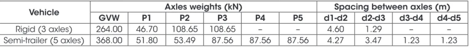
The B-WIM system was calibrated following COST 323 [8] report indications. Therefore, two trucks were used, one rigid with three
axles and another semi-trailer with ive axles. A total of 56 pas -sages were performed for the two lanes, with 17 pas-sages for lane 1 (South-North direction) and 19 passages for lane 2 (North-South direction). The trucks properties are shown in Table 1, with their weights indicated by static scale weighing.
Table 2 and Table 3 present the velocities and axles spacing ob-tained for the 17 passages on lane 1 and the 19 passages for lane
2, respectively, the errors of axles spacing for each passage when compared to the real values are also shown. It can be seen that the maximum absolute difference between the real spacing and the calculated one is 15 cm, which occurred in the second passage on lane 2, corresponding to a small error of just 3.25%. For the closed spaced axles, the highest errors are 6.17% and 6.19%, for lanes 1 and 2 respectively. Although this percentage is relatively high, these errors correspond to only 8 cm of difference between the real axle space and the calculated one.
The next step was to ilter the signal in order to obtain the actual IL and the weighing of the trafic vehicles. The structure fundamental
frequency was acquired by performing a frequency domain analy-sis in the free vibration part of the signals obtained during the pas-sage of the calibration trucks. The frequency domain response for each passage was attained from a Fast Fourier Transform (FFT), as can be seen in Figure 9. The value of 10 Hz can be assigned as the structure fundamental frequency.
The complete signals of each calibration event in the frequency domain are presented in Figura 10, where one can verify that frequencies up to 2.5 Hz are responsible for great part of the amplitude in the structure response. Thus, this value was
de-ined as the cut off frequency for the signal iltering. All passages signals were then iltered in frequency domain previously to the
weighing process.
Table 2
Velocities and axles spacings obtained with FAD sensors for lane 1
Passage Number of axles
Velocity (m/s)
Calculated axles spacings (m) Error (%)
d1-d2 d2-d3 d3-d4 d4-d5 d1-d2 d2-d3 d3-d4 d4-d5
1 3 22.34 4.67 1.31 – – -1.48 -1.47 – –
2 3 25.41 4.66 1.24 – – -1.41 3.82 – –
3 3 25.73 4.67 1.26 – – -1.60 2.61 – –
4 3 26.06 4.63 1.27 – – -0.69 1.36 – –
5 3 22.84 4.59 1.29 – – 0.12 -0.28 – –
6 3 23.64 4.66 1.29 – – -1.36 -0.18 – –
7 3 24.79 4.65 1.21 – – -1.04 6.17 – –
8 3 24.20 4.63 1.23 – – -0.69 4.75 – –
9 3 23.64 4.66 1.29 – – -1.36 -0.20 – –
10 3 25.09 4.66 1.23 – – -1.22 5.01 – –
11 3 18.15 4.64 1.24 – – -0.95 3.83 – –
12 3 18.15 4.64 1.28 – – -0.95 1.08 – –
13 5 21.62 4.27 3.51 1.27 1.27 0.10 -1.02 -3.00 -3.00
14 5 23.91 4.20 3.50 1.21 1.21 1.56 -0.95 1.27 1.27
15 5 23.91 4.30 3.46 1.26 1.21 -0.63 0.40 -2.54 1.27 16 5 24.79 4.21 3.53 1.21 1.26 1.36 -1.85 1.59 -2.34 17 5 23.64 4.20 3.55 1.20 1.25 1.62 -2.44 2.42 -1.32
Table 1
Properties of the trucks used during the calibration process
Vehicle Axles weights (kN) Spacing between axles (m)
GVW P1 P2 P3 P4 P5 d1-d2 d2-d3 d3-d4 d4-d5
With the iltered data, it was attained the IL for lane 1 and lane 2,
as shown on Figure 11, together with the theoretical IL. By
observ-ing this igure, three aspects can be highlighted: (i) calibration ILs
present peaks inferior to the theoretical IL; (ii) calibration ILs are bigger in extension than the theoretical one and; (iii) lane 1 IL
pres-ent an unexpected behavior, speciically near the South support. Related to the irst aspect, it is clear that the real support condi -tions are different from the idealized theoretical ones, occurring a smoothing in the IL maximum value.
The extension of the calibration ILs (second aspect) will always
be bigger than the bridge length, because the readings start on the instant in which the vehicle enters the bridge (Figure 01) and do not end right after it leaves. In the application of Moses’
method, when the irst axle enters the bridge (t = 0), the other axles do not cause deformation, but they need to be taken into account. Furthermore, because the load is dynamic, the effects caused by the passage of the vehicle do not cease after its exit from the structure. In fact, the structure still presents free vibra-tion response for a while. When this signal stretch is not consid-ered, higher errors occur. Thus, it was decided to extend the IL
Table 3
Velocities and axles spacings obtained with FAD sensors for lane 2
Passage Number of axles
Velocity (m/s)
Calculated axles spacings (m) Error (%)
d1-d2 d2-d3 d1-d2 d2-d3
1 3 24.56 4.70 1.25 – – -2.21 3.31 – –
2 3 24.56 4.75 1.30 – – -3.25 -0.43 – –
3 3 23.99 4.73 1.31 – – -2.89 -1.70 – –
4 3 23.72 4.72 1.30 – – -2.71 -0.55 – –
5 3 24.27 4.69 1.33 – – -2.04 -2.91 – –
6 3 24.27 4.69 1.33 – – -2.04 -2.91 – –
7 3 24.86 4.71 1.31 – – -2.38 -1.64 – –
8 3 24.56 4.75 1.30 – – -3.25 -0.43 – –
9 3 24.56 4.70 1.30 – – -2.21 -0.41 – –
10 3 24.27 4.69 1.28 – – -2.04 0.76 – –
11 3 18.76 4.73 1.28 – – -2.74 0.60 – –
12 3 23.45 4.72 1.33 – – -2.54 -2.97 – –
13 5 25.79 4.28 3.53 1.26 1.26 -0.28 -1.62 -2.39 -2.37 14 5 24.86 4.27 3.54 1.26 1.26 -0.07 -2.14 -2.65 -2.63 15 5 25.79 4.28 3.58 1.26 1.26 -0.28 -3.07 -2.39 -2.39 16 5 15.51 4.27 3.51 1.24 1.24 -0.06 -1.29 -1.00 -1.00 17 5 24.86 4.32 3.54 1.26 1.21 -1.20 -2.15 -2.63 1.31 18 5 21.72 4.33 3.52 1.31 1.23 -1.33 -1.47 -6.90 -0.02 19 5 17.05 4.26 3.53 1.27 1.23 0.16 -1.74 -2.90 -0.19
Figure 9
Fundamental frequency of the structure obtained
experimentally
Figure 10
length beyond the bridge ends. It was observed that this
exten-sion directly inluences the preciexten-sion of the acquired weights.
The extension must be adjusted case by case. For the bridge here analyzed, it was found the value of 36 m for the total exten-sion as the one leading to lower relative errors.
The characteristics of the IL of lane 1, both in terms of shape and
maximum value, have occurred due the large oscillation present in the signals originated by the presence of defects in the South
entrance of the bridge. In this case, the iltering process was not
effective to minimize the dynamic effects.
Using the obtained ILs, the axles weights and GVW of the cali-bration vehicles were calculated as described on item 2. Table 4
Figure 11
Comparison between ILs acquired during the B-WIM system calibration and the theoretical one
Table 4
Errors (%) acquired for the passages of the calibration vehicles on lane 1
Passage P1 P2 P3 P4 P5 GVW
1 -5.65 -12.91 11.61 – – -1.53
2 -43.59 147.09 -126.97 – – 0.57
3 -51.18 162.49 -142.75 – – -0.93
4 -47.67 128.14 -114.96 – – -3.01
5 -28.02 32.26 -26.39 – – -2.54
6 -23.10 61.20 -62.53 – – -4.63
7 -34.92 119.64 -110.40 – – -2.37
8 -21.15 90.92 -85.44 – – -1.48
9 -15.05 49.23 -51.42 – – -3.56
10 -33.40 109.00 -94.78 – – -0.06
11 -70.71 -5.24 56.76 – – 8.70
12 -73.72 1.24 50.42 – – 8.22
13 -43.31 80.15 -684.41 954.71 -324.55 2.75
14 11.14 -0.04 -79.57 30.72 42.71 0.08
15 -27.23 48.09 -241.83 188.07 15.18 0.22
16 -14.17 27.09 -54.20 -66.16 87.91 -1.98
17 2.12 13.72 -167.98 146.13 15.57 2.29
Absolute
and Table 5 bring the errors for axles weights and GVW for each passage during the calibration process when compared to the
data in Table 1. Although the calibration vehicles had signiicantly
different GVWs, the errors were compared together because the system must be robust in order to weigh vehicles with different
characteristics with a certain conidence margin. As can be seen,
the errors for individual axles weight are high, especially for the closed spaced ones. On the other hand, in relation to GVW, the errors are smaller, with maximum error of 8.70% for lane 1 and 3.17% for lane 2, and relative medium error inferior of 3% for both cases.
3.3 Traic characterization
Figure 12 illustrates the vehicles histogram, based on number of axles, that crossed over Lambari bridge during the 42 days of
monitoring. Vehicles up to three axles summed 52% of total trafic.
The GVW of those vehicles, as expected, did not show high values as can be seen in the GVW histogram shown in Figure 13. For this histogram, it is also possible to observe that GVW superior to 300 kN were given by trucks with 6-axle and above which were respon-sible for the upper tail of the distribution.
The histograms of maximum bending moment at midspan are
Table 5
Errors (%) acquired for the passages of the calibration vehicles on lane 2
Passage P1 P2 P3 P4 P5 GVW
1 -1.42 12.02 -9.57 – – 0.76
2 -3.07 6.45 -7.66 – – -1.04
3 12.02 -18.53 14.32 – – 0.39
4 6.04 -16.34 14.34 – – 0.25
5 14.17 -7.64 4.20 – – 1.09
6 10.16 -4.44 2.41 – – 0.96
7 -3.52 9.38 -7.47 – – 0.16
8 5.00 2.71 -4.64 – – 0.09
9 2.25 -1.95 2.25 – – 0.52
10 2.60 9.51 -7.02 – – 1.48
11 -0.64 -9.99 14.14 – – 1.60
12 -2.64 -14.74 14.91 – – -0.40
13 -9.07 12.88 -86.10 116.08 -50.66 -2.34
14 0.13 9.07 -108.78 150.44 -58.35 -1.28
15 -6.12 16.98 -118.92 153.52 -62.74 -2.54
16 23.14 -42.22 237.69 -354.22 166.61 3.12
17 24.20 -15.29 -89.10 198.10 -105.49 0.02
18 13.20 -10.95 -31.11 71.07 -35.29 -0.05
19 27.47 -55.37 284.48 -388.59 167.11 3.17
Absolute
medium error 8.78 14.55 55.74 75.37 34.01 1.11
Figure 12
Vehicles histogram, based on number of axles,
that traveled over Lambari bridge
Figure 13
presented in Figure 14 for each girder. The histograms for girders V3 and V4 show higher dispersion of results when compared to the ones for girders V1 and V2. This happened due to the defects in the South entrance, leading the vehicles to generate more impact when entering the bridge, as can be observed also in lane 1 IL. The central girders, V2 and V3, were the most loaded ones,
show-ing that trafic lowed close to the longitudinal axis of the bridge.
For these girders, Figure 15 shows the bending moment histogram for each vehicle with more than 3 axles. As can be seen, vehicles
with 3, 4 and 5 axles contributed signiicantly to the upper tail of the
distribution, presenting maximum bending moments in the same magnitude as the ones introduced by vehicles with 6 or more axles.
Figure 16 presents the dynamic ampliication factor for each ve -hicle that traveled over the bridge during the 42 days of monitoring. It is observed that trucks with lower GVW present higher impact
coeficient values, identifying an inversely proportional relation -ship between GVW and DAF. This behavior is in agreement with what was observed by [38]. Fitting a Fréchet distribution to the
measured cumulative probability distribution, as shown in Figure 16 (b), a value of 1.31 for DAF is obtained. This value is in agree-ment with the one indicated in the Brazilian Code NBR 7188 [40] for the analyzed bridge (1.33).
4. Conclusions
In the present study, results of the monitoring of a reinforced con-crete bridge in Goiás State by means of a B-WIM system are
pre-sented. From these data, it can be concluded about the application of such system:
n The adopted procedure to acquire the Inluence Line, implement -ed in the B-WIM system [31], has made possible to obtain the ac-tual IL of the structure, representing the real support conditions.
n The FAD system for vehicle classiication proved to be ef
-icient in detecting the axles of the vehicles traveling alone
on the bridge. However, when there is multiple presence this procedure is not recommended. If there is a need for accurate
Figure 14
classiication of vehicles, image data must be used, so a 3-axle vehicle, e.g., can be classiied either as a bus or a truck.
n The system provided good estimation of GVW. On the other hand, weight of isolated axles showed great variability. As a result, this study provided an indication that for the bridge
ana-lyzed, and the B-WIM system employed, only the trafic com -position (silhouettes and velocities) and the GVW of vehicles could be adequately obtained.
From the monitoring data, it was possible to characterize the active
trafic in the logistic corridor studied and its impact on the bridge inter -nal forces. From this a-nalysis, the following conclusions are drawn:
n Vehicles with up to three axles made up more than half of the
trafic during the period of monitoring.
n The vehicles tended to travel next to the longitudinal axis of the bridge instead of on rolling lanes, inducing greater stresses in the central girders.
n Even vehicles with relatively low GVW have introduced high
stresses due to their higher dynamic ampliication factor.
Figure 15
Bending moments histogram for girders V2 and V3 by means of vehicle class
Figure 16
(a) Dynamic ampliication factor (DAF) by vehicle type and (b) itting a Fréchet function to the
cumulative probability of DAF
B
B
B
5. Acknowledgements
The authors would like to thank the Transport Infrastructure
Na-tional Department (DNIT) for the inancial support and to the Foun -dation of Research Support and University Extension (FAPEU) and to the Foundation for Socioeconomic Studies (FEPESE) for the scholarships.
6. References
[1] ASSOCIAÇÃO BRASILEIRA DE NORMAS TÉCNICAS. Cargas móveis em pontes rodoviárias. NB-6, Rio de Janeiro, 1960.
[2] Žnidarič A. Kreslin M. Lavrič I. Kalin J. Simpliied approach to modelling trafic loads on bridges. Procedia – Social and
Behavioral Sciences, v.48, 2012, p.2887-2896.
[3] O’Brien E. Žnidarič A. Ojio T. Bridge Weigh-in-Motion – latest
developments and applications world wide. In: International Conference of Weigh-in-Motion, 5th, Paris, 2008, p.25-38. [4] Moses F. Weigh-in-Motion system using instrumented
bridg-es. ASCE Transp Eng J, v.105, n.3, 1979, p.233-249. [5] Peters RJ. AXWAY - A system to obtain vehicle axle weigths.
In: Conference of the Australian Road Research Board, 12th, Hobart, 1984, p.19-29.
[6] Peters RJ. CULWAY - an unmanned and undetectable high-way speed vehicle weighing system. In Conference of the Australian Road Research Board, 13th, Adelaide, 1986, p.70-83.
[7] O’Brien EJ. Žnidarič A. Weigh-in-Motion of Axles and Ve -hicles for Europe (WAVE). Report of Work Package 1.2: Bridge WIM systems (B-WIM), 2001, 100 p.
[8] COST 323–Weigh-in-Motion of Road Vehicles - Final
Re-port. Appendix 1: European WIM Speciication, 1999.
[9] Jacob B. Weigh-in-motion of Axles and Vehicles for Eu-rope (WAVE) - General Report. 4th Framework Programme Transport. RTD project, RO-96-SC, 403, 2001.
[10] Yamada K. Ojio T. Bridge weigh-in-motion system using re-action force method. In: International Workshop on Structur-al HeStructur-alth Monitoring of Bridges/Colloquium on Bridge Vibra-tion, Japan Society of Civil Engineers, 2003, p.269-276. [11] Yu Y. Cai C. Deng L. State-of-the-art review on bridge
weigh-in-motion technology. Advances in Structural Engineering, v.19, n.9, 2016, p.1514-1530.
[12] Jiang RJ. Au FTK. Cheung YK. Identiication of vehicles
moving on continuous bridges with rough surface. Journal of Sound and Vibration, v.274, 2004, p.1045-1063.
[13] Au FTK. Jiang RJ. Cheung YK. Parameter identiication of
vehicles moving on continuous bridges. Journal of Sound and Vibration, v.269, 2004, p.91-111.
[14] Law SS. Bu JQ. Zhu XQ. Chan SL. Vehicle Condition Sur-veillance on Continuous Bridges Based on Response Sensi-tivity. Journal of Engineering Mechanics, v.132, n.1, 2006, p.78-86.
[15] Deng L. Cai CS. Identiication of parameters of vehicles
moving on bridges. Engineering Structures, v.31, n.10, 2009, p.1514-1530.
[16] Pan C. Yu L. Moving force identiication based on irely al -gorithm. Advanced Materials Research, v. 919, n.1, 2014, p.329-333.
[17] Kim S. Lee J. Park M. Jo B. Vehicle Signal Analysis Using
Artiicial Neural Networks for a Bridge Weigh-in-Motion Sys -tem. Sensors, v.9, 2009, p.7943-7956.
[18] Leming SK. Stalford HL. Bridge weigh-in-motion system de-velopment using superposition of dynamic truck/static bridge interaction. In: American Control Conference, Denver, 2003. [19] Law SS. Bu JQ. Zhu XQ. Chan SL. Vehicle axle loads
identi-ication using inite element method. Engineering Structures,
v.26, 2004, p.1143-1153.
[20] González A. Rowley C. O’Brien EJ. A general solution to the
identiication of moving vehicle forces on a bridge. Int. J. Nu -mer. Meth. Engng, v.75, 2008, p.335-354.
[21] Rowley CW. O’Brien EJ. González A. Žnidarič A. Experimen
-tal Testing of a Moving Force Identiication
BridgeWeigh-in-Motion Algorithm. Experimental Mechanics, v. 49, 2009, p.743-746.
[22] Deesomsuk T. Pinkaew T. Effectiveness ofVehicleWeight Estimation from BridgeWeigh-in-Motion. Advances in Civil Engineering, 2009, p.1-13.
[23] Karoumi R. Wiberg J. Liljencrantz A. Monitoring trafic loads
and dynamic effects using an instrumented railway bridge. Engineering Structures, v.27, n.12, 2005, p.1813-1819. [24] Carvalho Neto JA. Veloso LACM. Weighing in motion and
characterization of the railroad trafic with using the B-WIM
technique. Ibracon Structures and Materials Journal, v.8, n.4, 2015, p.491-506.
[25] Žnidarič J. Žnidarič A. Evaluation of the carrying capacity of
existing bridges – Final Report. Institute for Testing and Re-search in Materials and Structures, Ljubljana, 1994.
[26] Žnidarič A. Baumgartner W. Bridge Weigh-in-Motion sys -tems – an overview. In: European Conference of Weigh-in-Motion of Road Vehicles, 2nd, Lisbon, 1998, p.139-152.
[27] McNulty P. Testing of an Irish Bridge Weigh-in-Motion System, Dublin, 1999, Thesis (Master) - University College Dublin.
[28] González A. O’Brien EJ. Inluence of Dynamics on Accu -racy of a Bridge Weigh-in-Motion System. In: Conference of Weigh-in-Motion, 3rd, Orlando, 2002.
[29] McNulty P. O’Brien EJ. Testing of Bridge Weigh-in-Motion System in a Sub-Artic Climate. Journal of Testing and Evalu-ation, v.31, n.6, 2003.
[30] Quilligan M. Bridge Weigh-in-Motion: Development of a 2-D Multi-Vehicle Algorithm, Stockolm, 2003, Thesis (Phd) - Structural Design and Bridge Division, Royal Institute of Technology, 160 p.
[31] O’Brien EJ.Quilligan M. Karoumi R. Calculating an inluence
line from direct measurements. In: ICE Bridge Engineering, v.159, n.1, 2005, p.31-34.
[32] JungesP. Pinto RCA. Fadel Miguel LF. Linha de inluência
real de pontes utilizando sistemas BWIM. In: Congresso Brasileiro do Concreto, 56°, Anais, Natal, 2014.
[33] Ieng S. Bridge inluence line estimation for Bridge
[34] Heinen S. Pinto RCA. Fadel Miguel LF. Junges P. Effect of
transverse load distribution on the inluence lines given by a
bridge weigh in motion system. In: International Conference on Bridge Maintenance, Safety and Management, 8th, Anais,
Foz do Iguaçu, 2016.
[35] Žnidarič A. Žnidarič J. Terčelj S. Determination of the true trafic load in the process of safety assessment of existing
bridges. In: Congress of Structural Engineers of Slovenia, 12th, Anais, 1991, p.241-246.
[36] ISWIM. Weigh-in-Motion of Road Vehicles, 2013.
[37] Žnidarič A. Lavrič I. Kalin J. The next generation of bridge
weigh-in-motion systems. In: International Conference of Weigh-in-Motion, 3rd, 2002.
[38] ARCHES. Deliverable D10: Recommendations on dynamic
ampliication allowance, (2009).
[39] Gonzalez RC. Woods RE. Digital image processing. Pear-son, 3ed, 2007, 976 p.