Core-softened fluids, water-like anomalies, and the liquid-liquid critical
points
Evy Salcedo, Alan Barros de Oliveira, Ney M. Barraz, Charusita Chakravarty, and Marcia C. Barbosa
Citation: J. Chem. Phys. 135, 044517 (2011); doi: 10.1063/1.3613669
View online: http://dx.doi.org/10.1063/1.3613669
View Table of Contents: http://jcp.aip.org/resource/1/JCPSA6/v135/i4
Published by the American Institute of Physics.
Additional information on J. Chem. Phys.
Journal Homepage: http://jcp.aip.org/
Journal Information: http://jcp.aip.org/about/about_the_journal
Top downloads: http://jcp.aip.org/features/most_downloaded
Core-softened fluids, water-like anomalies, and the liquid-liquid
critical points
Evy Salcedo,1,a)Alan Barros de Oliveira,2,b) Ney M. Barraz, Jr.,3,c)
Charusita Chakravarty,4,d)and Marcia C. Barbosa5,e)
1Departamento de Física, Universidade Federal de Santa Catarina, Florianópolis, SC, 88010-970, Brazil
2Departamento de Física, Universidade Federal de Ouro Preto, Ouro Preto, MG, 35400-000, Brazil
3Programa de Pós-graduação em Física da UFRGS, Bento Gonçalves 9500, 91501970, Porto Alegre,
RS, Brazil
4Department of Chemistry, Indian Institute of Technology-Delhi, New Delhi 110016, India
5Instituto de Física, Universidade Federal do Rio Grande do Sul, Porto Alegre, RS, 1501-970, Brazil
(Received 4 March 2011; accepted 28 June 2011; published online 29 July 2011)
Molecular dynamics simulations are used to examine the relationship between water-like anomalies and the liquid-liquid critical point in a family of model fluids with multi-Gaussian, core-softened pair interactions. The core-softened pair interactions have two length scales, such that the longer length scale associated with a shallow, attractive well is kept constant while the shorter length scale associated with the repulsive shoulder is varied from an inflection point to a minimum of progres-sively increasing depth. The maximum depth of the shoulder well is chosen so that the resulting potential reproduces the oxygen-oxygen radial distribution function of the ST4 model of water. As the shoulder well depth increases, the pressure required to form the high density liquid decreases and the temperature up to which the high-density liquid is stable increases, resulting in the shift of the liquid-liquid critical point to much lower pressures and higher temperatures. To understand the entropic effects associated with the changes in the interaction potential, the pair correlation entropy is computed to show that the excess entropy anomaly diminishes when the shoulder well depth in-creases. Excess entropy scaling of diffusivity in this class of fluids is demonstrated, showing that decreasing strength of the excess entropy anomaly with increasing shoulder depth results in the pro-gressive loss of water-like thermodynamic, structural and transport anomalies. Instantaneous normal mode analysis was used to index the overall curvature distribution of the fluid and the fraction of imaginary frequency modes was shown to correlate well with the anomalous behavior of the diffu-sivity and the pair correlation entropy. The results suggest in the case of core-softened potentials, in addition to the presence of two length scales, energetic, and entropic effects associated with local minima and curvatures of the pair interaction play an important role in determining the presence of water-like anomalies and the liquid-liquid phase transition.© 2011 American Institute of Physics. [doi:10.1063/1.3613669]
I. INTRODUCTION
Water is characterized by well-known thermodynamic and kinetic liquid-state anomalies; for example, the rise in density on isobaric heating (density anomaly) and the in-crease in molecular mobility on isothermal compression (dif-fusivity anomaly).1 Since the anomalies of bulk water are
connected with its behavior as a solvent in chemical and biological systems, an understanding of the structural ori-gins of such anomalous behavior has attracted considerable attention.2,3While the anomalies of water were initially
pre-sumed to be uniquely connected to the hydrogen-bonded net-work of water,4there is now evidence that a number of liquids
display water-like liquid-state anomalies, such as Te,5 Ga,
Bi,6S,7,8Ge
15Te85,9silica,10–12silicon,13and BeF2.10,11,14,15
a)Electronic mail: [email protected]. b)Electronic mail: [email protected]. c)Electronic mail: [email protected]. d)Electonic mail: [email protected]. e)Electronic mail: [email protected].
The generic relationships between structure, entropy and mo-bility underlying this diverse set of liquids with water-like anomalies, can be understood in terms of the behavior of the excess entropy (Sex), defined as the difference between the entropy (S) of the liquid and the corresponding ideal gas at the same density and temperature.11,16–23 A
neces-sary condition for the fluid to show density, diffusion, and structural anomalies is the presence of anomalous excess en-tropy behavior, corresponding to a rise in Sexon isothermal compression (∂Sex/∂ρ >0).11,14,15,21–25 The structural basis for the excess entropy anomaly is the existence of distinct forms of local order or length scales in the low- and high-density regimes; competition between the two types of lo-cal order results in a rise in excess entropy at intermediate densities.
In addition to the singularity-free scenario for water-like thermodynamic and kinetic anomalies, it has been conjec-tured that the anomalies of water are due to the presence of a second liquid-liquid critical point, corresponding to the onset of a line of first-order phase transitions between
044517-2 Salcedoet al. J. Chem. Phys.135, 044517 (2011)
high- and low-density phases of water.26The relationship be-tween the liquid-liquid critical point and water-like anoma-lies can be addressed by considering minimal models of liquids with isotropic, pair-additive interactions that give rise to water-like anomalies, as well as liquid-liquid criti-cal points.27–30 Such simple models are able to capture
sev-eral water features, including liquid-liquid phase transition, thermodynamic, and dynamic anomalies,31–35 yet amenable
analytically.36–39While two length scales in the pair
interac-tion appears to be a necessary condiinterac-tion for seeing both the liquid-liquid critical point (LLCP) and water-like anomalies, it is possible to design isotropic potentials with two length scales where appropriate variation of parameters can result in shifting either the LLCP or the water-like anomalies into the metastable or unstable regime.40In this paper, we study a family of liquids with continuous and core-softened pair in-teractions consisting of a hard core, a short-range shoulder, and an attractive well at a larger separation.40 Since the
po-tentials share a common functional form consisting of a sum of one Lennard-Jones and four Gaussian terms, we refer to them as the family of multi-Gaussian water-like liquids. By suitably varying the parameters, the outer attractive well can be left unchanged, while the shoulder can be progressively altered from being purely repulsive to a deep attractive well. As the shoulder shifts from being purely repulsive to more attractive, the anomalous regime in the pressure-temperature plane shrinks and disappears while the LLCP shifts to higher temperatures and lower pressures. The connection with atom-istic models is made by ensuring that the limiting case of the double minimum potential that has no anomalies corresponds to an isotropic potential that reproduces the oxygen-oxygen radial distribution function of ST4 water.41 Using this set of
anomalous fluids, we address a number of questions related to the features of the pair interaction, in addition to the two length scales, that control the temperature-pressure regime of the water-like liquid state anomalies versus the liquid-liquid critical point. Both the liquid-liquid critical point and the water-like anomalies require a change in the nature of local or-der in the liquid with density, and therefore two length scales in the case of core-softened fluids. The liquid-liquid critical point, however, depends on the energetic bias towards segre-gation of the two length scales with decreasing temperature. In contrast, the water-like liquid state anomalies require an excess entropy anomaly, involving a continuous transforma-tion of the liquid from low- to high-density through a range of quasi-binary states reflecting the competition between two length scales in the intermediate regime.18 In order to
under-stand the relationship between the interaction potential, the water-like liquid state anomalies and the liquid-liquid critical point, it is therefore necessary to consider the temperature-dependent stabilization of the low- and high-density length scales as well as the density-dependent changes in the entropy of the system.
In order to understand how the change in interaction po-tential within the multi-Gaussian water models affects the thermodynamic and kinetic water-like anomalies, it is neces-sary to map out the excess entropy anomaly for the different model fluids. We use the pair correlation entropy as a sim-ple structural estimator of the excess entropy, defining it for a
one-component fluid of structureless particles as
S2 N kB = −
2πρ
∞
0 {
g(r) lng(r)−[g(r)−1]}r2dr, (1)
where g(r) is the radial distribution function. It is typically the dominant contribution to the excess entropy of a fluid expressed as a multi-particle correlation expansion of the form
Sex=S−Sid=S2+S3+. . . , (2)
whereSnis the entropy contribution due ton-particle spatial
correlations.42–46 The excess entropy and mobility anomalies
are linked by excess entropy scaling relations of the form
X∗=Aexp(α(Sex/N kB)), (3)
where X∗ are dimensionless transport properties with either macroscopic (Rosenfeld) or microscopic (Dzugutov) reduc-tion parameters and the scaling parameters,αandA, depend on the functional form of the underlying interactions.47–50
In the case of simple liquids, the excess entropy scaling pa-rameters can be approximately set as A≈0.6 and α≈0.8. In addition, for such fluids, the pair correlation entropy per particle,s2, typically represents 85%−90% of the total ex-cess entropy.51 Mittal et al. investigated the approximation
Sex≈S2 as well as the relation between the excess entropy and the diffusion coefficient for the specific case of core-softened fluids.20,22 They have shown that S
2 captures the most important and qualitative behaviors of Sex with a rea-sonable quantitative accuracy.
As an additional means to relate the interaction poten-tial to the liquid-state properties, we characterize the potenpoten-tial energy surface (PES) of the multi-Gaussian family of water-like liquids using instantaneous normal mode analysis. In the instantaneous normal mode (INM) approach, the key quan-tity is the ensemble-averaged curvature distribution of the PES sampled by the system. For a system of N particles, the mass-weighted Hessian associated with each instanta-neous configuration is diagonalized to yield 3N normal mode eigenvalues and eigenvectors and the ensemble-average of this distribution is referred to as the INM spectrum. The INM spectrum of a liquid will have a substantial fraction of unsta-ble modes with negative eigenvalues that simulations suggest is strongly correlated with the diffusivity.52–57Random energy
models of liquids also suggest that for supercooled liquids there will be a connection between the fraction of imaginary modes, the diffusivity, and the configurational entropy.58,59 Our previous work on INM analysis of a core-softened water-like fluid demonstrated that the instantaneous normal mode spectra carry significant information on the dynamical conse-quences of the interplay between length scales characteristic of anomalous fluids.19 We have therefore performed an INM
analysis of the multi-Gaussian water-like fluids to understand the relationship between the interaction potential, anomalies and the liquid-liquid critical point.
1.2 1.8 2.4 3.0 r*
0 4 8
U*
A case B case C case D case
FIG. 1. Interaction potential obtained by changing parametersh1in Eq.(4).
The potential and the distances are in dimensionless unitsU∗=U/γ and r∗=r/r0.
II. THE MODEL
A. The potential
The multi-Gaussian family of water-like fluids is defined by pair-additive, continuous, and core-softened interactions with the functional form
U(r)=ǫ σ
r a
−σ
r b
+ 4
j=1 hjexp
− r−cj
wj
2 .
(4)
The first term is a Lennard-Jones potential-like and the second one is composed of four Gaussians, each of widthwj
centered atcj. The potential and the distances are given in
di-mensionless units,U∗=U/γ andr∗=r/r
0, whereγ is the energy scale andr0is the length scale chosen so the closest approach between particles is about r∗ =1, i.e., so that the second length scale associated with the repulsive shoulder re-mains the same. Here we use ǫ/γ =0.02 andσ/r0 =1.47. Modifyingh1in the Eq.(4)allows us to change the depth of the hard-core well, as illustrated in Fig.1while keeping the shape and location of the attractive well constant. We report here results for four different values forh1 and they are ex-pressed as a multiple of a reference valuehref1 as shown in the TableI. For all the four cases the values ofa, b,{cj, wj}with
j =1, . . . ,4, and href. Table IIgives the parameter values in Å and kcal/mol consistent with reproducing the oxygen-oxygen radial distribution of ST4 water using case D.41
TABLE I. Parametersh1for potentials A, B, C, and D.
Potential Value ofh1
A 0.25href1
B 0.50href1
C 0.75href1
D 1.00href1
TABLE II. Parameters for potentials A, B, C, and D in units of Å and of kcal/mol.
Parameter Value Parameter Value
a 9.056 w1 0.253
b 4.044 w2 1.767
ǫ 0.006 w3 2.363
σ 4.218 w4 0.614
c1 2.849 href1 −1.137
c2 1.514 h2 3.626
c3 4.569 h3 −0.451
c4 5.518 h4 0.230
B. The simulation details
The properties of the system were obtained by NVT molecular dynamics using Nose-Hoover heat-bath with cou-pling parameter Q=2. The system is characterized by 500 particles in a cubic box with periodic boundary conditions, interacting with the intermolecular potential described above. All physical quantities are expressed in reduced units and de-fined as
t∗= t(m/γ) 1/2 r0
T∗= kBT γ
p∗= pr0 γ
ρ∗=ρr03
D∗= Dm
γ r02 . (5)
Standard periodic boundary conditions together with predictor-corrector algorithm were used to integrate the equa-tions of motion with a time step t∗=0.002 and potential cut off radius rc∗=3.5. The initial configuration is set on solid or liquid state and, in both cases, the equilibrium state was reached after teq∗ =1000 (what is in fact 500 000 steps since t∗=0.002) . From this time on the physical quantities were stored in intervals of t∗
R =1 during tR∗ =1000. The
sys-tem is uncorrelated aftert∗
d =10, as judged from the velocity
auto-correlation function. 50 decorrelated samples were used to get the average of the physical quantities.
At each state point, 100 configurations were sampled and used to construct the instantaneous normal mode spectra and associated quantities. We repeated the calculation for some state points using 500 configurations and found no significant difference.
C. Instantaneous normal modes analysis
The potential energy of configuration rnear r0 can be
written as a Taylor expansion of the form
U(r)=U(r0)−F•z+
1 2r
T
044517-4 Salcedoet al. J. Chem. Phys.135, 044517 (2011)
wherezi=√mi(ri−r0) are the mass-scaled position
coordi-nates of a particlei. The first and second derivatives ofU(r) with respect to the vectorzare the force and the Hessian ma-trix, denoted by F and H, respectively. The eigenvalues of the HessianHare ({ω2i}, i=1,3N) representing the squares of normal mode frequencies, andW(r) are the corresponding eigenvectors. In a stable solid, r0 can be conveniently taken
as the global minimum of the potential energy surfaceU(R), which implies that F=0 andHhas only positive
eigenval-ues corresponding to oscillatory modes. The INM approach for liquids interpretsras the configuration at timet relative to the configuration r0 at time t0. Since typical
configura-tions,r0are extremely unlikely to be local minima, therefore F=0 and H will have negative eigenvalues. The negative
eigenvalue modes are those which sample negative curva-ture regions of the PES, including barrier crossing modes. The ensemble-averaged INM spectrum,f(ω), is defined as
f(ω)=
1 3N
3N
i=1
δ(ω−ωi)
. (7)
Quantities that are convenient for characterizing the instanta-neous normal mode spectrum are: (i) the fraction of imaginary frequencies (Fi), defined as
Fi=
im
f(ω)dω, (8)
and the Einstein frequency (ωE), given by
ωE2 =
ω2f(ω)dω= T rH
m(3N−3), (9)
where the integral is performed over the entire range of fre-quencies, real as well as imaginary.
III. RESULTS
A. Phase diagram
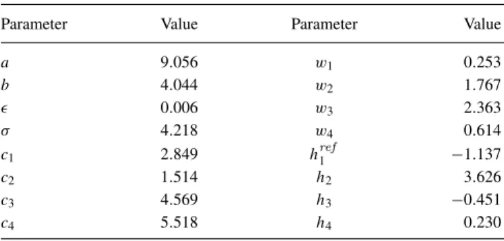
Figure 2 illustrates the pressure-temperature phase dia-gram for the four cases of the potential.40 Because of the
presence of the attractive interaction, all four cases have a liquid-gas transition with an associated critical point that is not shown here. In addition, all the four model liquids studied here have a liquid-liquid critical point. Cases A, B, and C have water-like density and diffusional anomalies. The solid bold lines represent the locus of temperatures of maximum den-sity (TMD) for different isobars. State points enclosed by the TMD locus represent the regime of density anomaly within which (∂ρ/∂T)P >0. The maximum temperature along the
TMD locus, denoted by TT MDmax , is the threshold temperature for onset of the density anomaly. The dotted-dashed lines are the temperatures of maximum and minimum diffusivity along different isotherms.40
This overall change in the nature of the liquid-state phase diagram for the four multi-Gaussian liquids is summarized in Figure 3. Clearly, as the second length scale shifts from an inflection point on the repulsive shoulder to a well with pro-gressively increasing depth and curvature, the region of liq-uid state anomalies shrinks and disappears. The figure illus-trates how the pressure and temperature associated the
liquid-0.2 0.4 0.6 0.8 1.0
T*
0 2 4
p*
A case
0.2 0.4 0.6 0.8 1.0
T*
-1 0 1 2 3
p*
B case
0.4 0.6 0.8 1.0
T*
-1 -0.5 0 0.5 1
p*
C case
0.6 0.8 1.0
T*
-0.9 -0.6 -0.3 0
p*
D case
FIG. 2. Pressure-temperature phase diagram for cases A, B, C,and D. The thin solid lines are the isochores 0.30< ρ∗<0.65. The liquid-liquid critical
point is the dot, the locus of temperatures of maximum density is the solid thick line and the locus of diffusion extrema is the dot-dashed line.
gas and liquid-liquid critical points vary with the potentials A,B,C,and D. The same graph also shows that as the shoul-der becomes deeper, the maximum temperature of the TMD locus, which marks the onset temperature for thermodynam-ically anomalous behavior, approaches the liquid-liquid criti-cal point.
Since the thermodynamic and mobility anomalies of wa-ter are correlated, we first focus on understanding the thermo-dynamic condition for the presence of density anomaly. This may be stated as
∂S ∂ρ = −
V2α N KT
>0, (10)
where α is the thermal expansion coefficient and KT is the
isothermal compressibility. For the system to have a large
0.5 1.0 1.5 2.0 2.5
T* 0
1 2 3
p*
A case B case C case D case
A case - max of TMD B case - max of TMD C case - max of TMD
0.35 0.42 0.49 0.56
ρ∗
-4.0 -3.2 -2.4 -1.6
s 2
*
T* = 0.60 T* = 0.70 T* = 0.80 T* = 0.90 T* = 1.00 T* = 1.10
A case
0.35 0.42 0.49 0.56
ρ∗
-4.0 -3.2 -2.4 -1.6
s 2
*
T* = 0.60 T* = 0.70 T* = 0.80 T* = 0.90 T* = 1.00 T* = 1.10
B case
0.35 0.42 0.49 0.56
ρ∗
-4.0 -3.2 -2.4 -1.6
s 2
*
T* = 0.60 T* = 0.70 T* = 0.80 T* = 0.90 T* = 1.00 T* = 1.10
C case
0.35 0.42 0.49 0.56
ρ∗
-4.0 -3.2 -2.4 -1.6
s 2
*
T* = 0.60 T* = 0.70 T* = 0.80 T* = 0.90 T* = 1.00 T* = 1.10
D case
FIG. 4. Pair entropy versus density for the cases A, B, C, and D for various temperatures.
anomalous region, the ratio α/KT should be therefore large
and negative. Near the critical point, the compressibility,KT,
and thermal expansion coefficient, αT, diverge, however the
compressibility diverges with a large exponent making the ra-tio zero. In this case, the condira-tion given by Eq.(10)cannot be fulfilled. This suggests that near the liquid-liquid critical point the system prefers to undergo a phase separation into high- and low-density liquids rather than show a smooth en-tropy anomaly.
B. Excess entropy and pair correlations
As discussed in Sec. III A, the density anomaly corre-sponds to a set of state points for which (∂S/∂ρ)T >0. The
total entropy is a sum of the ideal (Sid) and excess (Sex) con-tributions. SinceSiddecreases monotonically with increasing density, therefore, a density anomaly must imply the pres-ence of an excess entropy anomaly, (∂Sex/∂ρ)T >0.
Erring-ton et al.have further shown that the strength of the excess entropy anomaly required to give rise to density anomaly is given by the conditionex=[∂(Sex/N kB)/∂lnρ]T >1.22
By approximating the excess entropy with the two-body cor-relation contribution ofs2 (see Eq. (1)), we relate the struc-tural information in the radial distribution function of the fluid to the thermodynamic behavior.
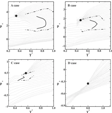
Figure 4 illustrates the s∗2(ρ)=S2/N kB versus ρ∗ for
various temperatures and for the potentials A,B,C,and D. For cases A,B, and C, at low temperatures, there is a rise in excess entropy on isothermal compression characteristic of water-like liquids11,19,20 that contrasts with the behavior of
simple liquids where free volume arguments are sufficient to justify a monotonic decrease in entropy on isothermal com-pression. For the case D, no anomaly is observed in the pair entropy even at low temperatures. The progressive attenuation of the anomalies on going from case A to caseD, is illustrated in Figure5which compares the behavior of the pair entropy versus density for all studied potentials at a given temperature, T∗ =0.9. This graph together with Figure3indicates that as the maximum temperature at the TMD line approaches the liquid-liquid critical temperature, the pair entropy curve be-comes more flat and the anomalous behavior disappears.
The origin of the pair entropy anomaly in fluids with two length scales can be explained in terms of a competition between two length scales at intermediate densities. Only a
0.32 0.40 0.48 0.56
ρ∗
-2.1 -1.8 -1.5
s*
A case B case C case D case
044517-6 Salcedoet al. J. Chem. Phys.135, 044517 (2011)
single length scale dominates in the low- and high-density limits while at intermediate densities, where both length scales are present, can be regarded as quasi-binary sys-tems with a mixing entropy. The radial distribution functions shown in our previous study clearly demonstrate the presence of two length scales. They also show that with the increasing temperature, the shorter length scale peak of g(r) becomes more prominent in cases A,B,and C. In contrast, in the case D, both length scales associated with the first and second peak of theg(r) broaden with increasing temperature as a conse-quence of which there is no emergence of an anomaly with decreasing temperature.
The crucial question to ask in the multi-Gaussian family of water models is why, despite the presence of two length scales at intermediate densities, the pair entropy anomaly is progressively lost as the shoulder goes from being an inflex-ion point to a minimum with about twice the depth as the outer, attractive well. Clearly the rise in entropy with isother-mal compression due to the mixing of two length scales is counteracted by additional effects. To understand this we note that the entropy of an one-dimensional harmonic oscillator of frequencyωis given by
sω
N kB =
1−ln(β¯ω). (11)
The increasing curvature of the short-range minimum, relative to the attractive minimum, implies that a pair-separated trapped in the shoulder minimum will have lower vibrational entropy than one trapped in the broad shallow at-tractive minimum. As a consequence, at intermediate densi-ties, while the presence of two length scales will increase entropy, the loss of entropy when the pairs are located in the short-range minimum will tend to decrease entropy. As the shoulder minimum becomes deeper, the second effect be-comes more important and the excess entropy anomaly dis-appears. In systems such as the two-scale linear ramp, such curvature-dependent effects will be absent.
It is also interesting to consider the shifting of the liquid-liquid critical point to lower pressures and higher tem-peratures. For a temperature-driven phase separation into low-density liquid (LDL) and high-density liquid (HDL), increasing energetic stabilization of one length scale relative to the other is required. In case A, this is clearly due to the outer attractive well with a depth of about U∗≈0.3 and T∗
c ≈0.3. In case D, this is due to the shorter length scale with
a well depth of about ∗=1.00 andT∗
c ≈0.8. For a
shal-low shoulder, the high density liquid is stabilized under high pressure. Within the HDL phase, particles are occupying the shoulder scale. The density anomalous region, characterized by having particles in the two scales occurs at the pressure range of the low density liquid phase. As the shoulder scale becomes deeper, less pressure is needed to form the high den-sity liquid. The LDL phase occupies a smaller pressure range and, therefore, the density anomalous region shrinks. For a very deep shoulder well as in case D, the HDL requires no pressure to be formed, the LDL is at negative pressures and the anomalous density regime disappears.
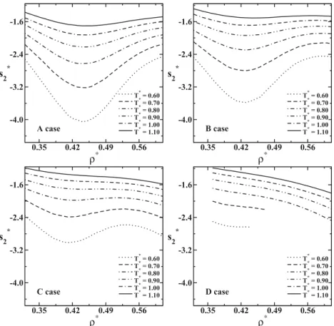
C. Diffusion and Rosenfeld reduction parameter
Previously we have shown that the diffusion coefficient in the cases A, B, and C decreases with the decrease of the density for a certain range of densities.40 The region in the
pressure temperature phase diagram limited by the maxima and minima of the diffusion coefficient is illustrated as dot-dashed lines in Fig.2. In the case D, the diffusion coefficient increases with the decrease of the density as in normal liq-uids. It is interesting to notice that the same behavior is also observed in the pair entropy suggesting that the anomalies present in these two quantities might be related. In order to check this hypothesis we now consider the scaling relation-ship between the diffusivity and the pair entropy. Using the Rosenfeld macroscopic reduction parameters for the length asρ−1/3and the thermal velocity as (k
BT /m)1/2, the
dimen-sionless diffusivity is defined as
DR ≡D
ρ1/3 (kBT /m)1/2
. (12)
The scaling of the reduced diffusivity,DR with pair entropy,
s∗
2 is illustrated in Fig.6. Previous results for core-softened fluids suggest that S=Sex−S2tends to be density depen-dent in anomalous fluids,16 resulting in a stronger isochores dependence when ln(DR) is plotted against S2, rather than against Sex. In the present study, we have computed onlyS2 and, therefore, Fig. 6 shows scaling with respect to S2. For case A, the collapse of data from all the state points on a sin-gle line is quite good. This case model very closely mimic those of the Gaussian-core fluid,60 a system which also
ex-hibits good scaling of Rosenfeld parameterized self diffusivity with two-body excess entropy. This makes logical sense since the case A and the Gaussian-core systems are qualitatively similar for low to intermediate temperatures. As we progress
0.8 1.6 2.4 3.2 4.0
-s2*
0.01 0.1
DR
ρ∗ = 0.30 ρ∗ = 0.35 ρ∗ = 0.40 ρ∗ = 0.45 ρ∗ = 0.50
A case
0.8 1.6 2.4 3.2 4.0
-s2*
0.01 0.1
DR
ρ∗ = 0.30 ρ∗ = 0.35 ρ∗ = 0.40 ρ∗ = 0.45 ρ∗ = 0.50
B case
0.8 1.6 2.4 3.2 4.0
-s2*
0.01 0.1
DR
ρ∗ = 0.35 ρ∗ = 0.40 ρ∗ = 0.45 ρ∗ = 0.50
C case
0.8 1.6 2.4 3.2 4.0
-s2*
0.01 0.1
DR
ρ∗ = 0.30 ρ∗ = 0.35 ρ∗ = 0.45 ρ∗ = 0.50 ρ∗ = 0.55 ρ∗ = 0.60
D case
FIG. 6. Diffusion in Rosenfeld units as a function of −s∗
2 for the cases
-40 -20 0 20 40 60
ω
0 0.03 0.06 0.09
f(ω)
A case
-40 -20 0 20 40 60
ω
0 0.03 0.06 0.09
f(ω)
B case
-40 -20 0 20 40 60
ω
0 0.03 0.06 0.09
f(ω)
C case
-40 -20 0 20 40 60
ω
0 0.03 0.06 0.09
f(ω)
D case
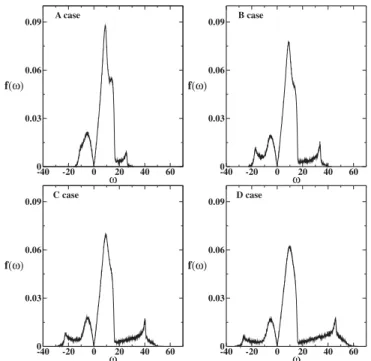
FIG. 7. Normal models versus frequency for the four studies cases. The den-sity is fixed,ρ∗=0.50 in all the cases and the temperature is varied.
from case A to case D, the isochores dependence of the scal-ing parameters becomes more pronounced suggestscal-ing that the density dependence of Sincreases on going from case A to case D.
This is consistent with other anomalous systems that were studied recently. For liquid water, the DR vs. s2 scal-ing holds reasonably well for lower temperature state points (where anomalies are present), but it develops clear iso-chore dependence at high temperature (where anomalies disappear).16,61For core-softened liquids with short-range
at-tractions theDRvs.s2relationship holds well for the anoma-lous state points and breaks down for conditions when the anomalies disappear.62–65
D. The instantaneous normal mode spectrum
The variation in anomalous behavior in the multi-Gaussian family of water-like liquids studied here suggests that in addition to length scales, we need to look at other fea-tures of the pair potential, e.g., its first and second derivatives. Instantaneous normal mode analysis provides a way to sum-marize information on the curvature distribution of the poten-tial energy landscape. In Figure7, we show the INM spectra of liquids bound by the four potentials (A, B, C, and D) at a common state point ofρ∗=0.50 and temperatureT∗=0.8. The crucial features are as follows:
0.3 0.4 0.5 0.6
ρ
∗0 0.05 0.10 0.15 0.20 0.25
F
iA case
0.3 0.4 0.5 0.6
ρ
∗0 0.05 0.10 0.15 0.20 0.25
F
iB case
0.3 0.4 0.5 0.6
ρ
∗0 0.05 0.10 0.15 0.20 0.25
F
iC case
0.3 0.4 0.5 0.6
ρ
∗0 0.05 0.10 0.15 0.20 0.25
F
iD case
FIG. 8. Fraction of imaginary modes versus density for fixed temperatures,T∗=0.20,0.30,0.40,0.50,0.60,0.70,0.80,0.90, and 1.10 from bottom to top for
044517-8 Salcedoet al. J. Chem. Phys.135, 044517 (2011)
• A low-frequency split peak in the real branch centered at about ω=10, that does not vary significantly be-tween the four cases and must reflect modes associated with the outer attractive well;
• A high-frequency peak in the real branch, centered at approximately 30, 35, 40, and 50 for cases A, B, C, and D, respectively, which must correspond to motion in neighborhood of the shoulder length scale. As the curvature of the short-range minimum increases, this features shifts to higher frequencies and becomes more prominent; and
• The imaginary branch reflects regions of negative cur-vature in the neighborhood of barriers and inflection points. Case A, where there is no barrier in the pair in-teraction but only an inflection point has a single peak such as a simple liquid. However, this peak is broad be-cause of the core-softened repulsive wall and the frac-tion of imaginary modes is large. As the barrier be-tween the short and long length scales becomes more pronounced in the pair interaction, the second peak in the imaginary branch becomes more prominent.
Thus, the real branch is dominated by vibrational modes associated with motion in the attractive and shoulder length scales while the imaginary modes branch is dominated by negative curvature modes associated with transitions between the shoulder and attractive wells. For the case A, the real branch has three peaks related to the three basins: the shoulder scale, the attractive scale, and a second attractive scale located at further distance in Fig. 1. It has just one imaginary peak that indicating that transitions between the two length scales do not require local barrier crossing. For the cases B and C, the imaginary branch has two peaks suggestive of modes con-necting between the shoulder scale, attractive scale, and sec-ond attractive scales. The peak with largest frequency in the real branch has larger frequency in the case C than in the case A and is related to the shoulder scale. For the case D, the shoulder is deep and so the frequency related to the shoul-der scale has a very high frequency. The imaginary branch has two distinct oscillation modes that exclude transitions be-tween the shoulder scale and the other scales and, therefore, no anomalies are expected.
The above discussion suggests that INM spectra carry fairly detailed information on the dynamics of transitions be-tween the two length scales. The two features which are a compact signature of INM spectra are the Einstein frequency and the fraction of imaginary modes. Isotherms of the Ein-stein frequency as a function of density for all the four cases show a monotonic increase with density and do not show any significant signatures of the water-like anomalies. The frac-tion of imaginary modes, in contrast, correlates strongly with the anomalous behavior of the pair entropy and the diffusiv-ity. Figure8 shows theFi curves versus density for various
isotherms of all the four multi-Gaussian model fluids stud-ied here. The parallel behavior of thes2(ρ) andFi(ρ) curves
at corresponding isotherms is immediately obvious, though theFi(ρ) have a stronger non-monotonic behavior thans2(ρ) curves. This can be seen most clearly for a high-temperature isotherm.
IV. CONCLUSIONS
This paper examines the relationship between water-like anomalies and the liquid-liquid critical point in a family of model fluids with multi-Gaussian and core-softened pair in-teractions. The pair interaction in this family of liquids is composed of a sum of Lennard-Jones and Gaussian terms, in such a manner that the longer length scale associated with a shallow, attractive well is kept constant while the shorter length scale associated with the repulsive shoulder changes from an inflection point to a minimum of progressively in-creasing depth. The maximum depth of the shoulder length scale is chosen so that the resulting potential reproduces the oxygen-oxygen radial distribution function of the ST4 model of water. As the energetic stabilization of the shoulder length scale increases, the liquid-liquid critical point shifts to higher temperatures and lower pressures. Simultaneously, the tem-perature for onset of the density anomaly decreases and the region of liquid state anomalies in the pressure-temperature plane diminishes. The condition for the presence of anoma-lies is inconsistent with divergences near a critical point, so that in the limiting case of maximum shoulder well depth, the anomalies disappear.
changes in vibrational entropy associated by the two length scales.
A general conclusion that emerges from this study is that even though the ratio between the two length scales is im-portant for locating the temperature range of the anomalies,66
additional energetic and entropic effects associated with lo-cal minima and curvatures of the pair interaction can play an important role. The liquid-liquid phase separation depends on the relative energies associated with the two length scales whereas the water-like anomalies depend upon a continuous rise in entropy as a function of isothermal compression. A number of recent studies of core-softened fluids illustrate this conclusion. For example, energetic and entropic effects play a very different role in the discrete and discontinuous ver-sions of the shouldered well potential.18 In the discrete case, the enthalpic implications do not change significantly and the liquid-liquid critical point is not significantly different in the two systems. In contrast, the continuous potential allows for a smooth transformation through a range of quasi-binary states from low- to high-density and shows water-like anomalies. A more recent study of core-softened fluids shows that increas-ing the depth of the attractive well,67while leaving the
shoul-der feature constant, results in disappearance of the anomalies while shifting the liquid-liquid critical point to lower pres-sures and higher temperatures.
ACKNOWLEDGMENTS
This work is supported by the Indo-Brazil Cooperation Program in Science and Technology of the CNPq (Brazil) and DST (India). This work is also partially supported by the CNPq through the INCT-FCx.
1O. Mishima and H. E. Stanley,Nature (London)396, 329 (1998).
2K. A. Dill, T. M. Truskett, V. Vlachy, and B. Hribar-Lee,Annu. Rev.
Bio-phys. Biomol. Struct.34, 173 (2005).
3P. Kumar, G. Franzese, and H. Eugene Stanley,J. Phys. Condens Matter
20, 244114 (2008).
4J. D. Bernal and B. H. Fowler,J. Chem. Phys.1, 515 (1933).
5H. Thurn and J. Ruska,J. Non-Cryst. Solids22, 331 (1976).
6See http://periodic.lanl.gov/default.htm, 2007 for periodic table of the
elements.
7G. E. Sauer and L. B. Borst,Science158, 1567 (1967).
8S. J. Kennedy and J. C. Wheeler,J. Chem. Phys.78, 1523 (1983).
9T. Tsuchiya,J. Phys. Soc. Jpn.60, 227 (1991).
10C. A. Angell, R. D. Bressel, M. Hemmatti, E. J. Sare, and J. C. Tucker,
Phys. Chem. Chem. Phys.2, 1559 (2000).
11R. Sharma, S. N. Chakraborty, and C. Chakravarty,J. Chem. Phys.125,
204501 (2006).
12P. H. Poole, M. Hemmati, and C. A. Angell,Phys. Rev. Lett.79, 2281
(1997).
13H. Tanaka,Phys. Rev. B66, 064202 (2002).
14M. Agarwal, R. Sharma, and C. Chakravarty,J. Chem. Phys.127, 164502
(2007).
15M. Agarwal and C. Chakravarty, J. Phys. Chem. B 111, 13294
(2007).
16M. Agarwal, M. Singh, R. Sharma, M. P. Alam, and C. Chakravarty,
J. Phys. Chem. B114, 6995 (2010).
17M. Agarwal, M. P. Alam, and C. Chakravarty,J. Phys. Chem. B115, 6935
(2011).
18A. B. de Oliveira, P. A. Netz, T. Colla, and M. C. Barbosa,J. Chem. Phys.
124, 084505 (2006).
19A. B. de Oliveira, E. Salcedo, C. Chakravarty, and M. C. Barbosa,J. Chem.
Phys.132, 234509 (2010).
20J. Mittal, J. R. Errington, and T. M. Truskett,J. Chem. Phys.125, 076102
(2006).
21J. Mittal, J. R. Errington, and T. M. Truskett,J. Phys. Chem. B110, 18147
(2006).
22J. R. Errington, T. M. Truskett, and J. Mittal,J. Chem. Phys.125, 244502
(2006).
23Z. Yan, S. V. Buldyrev, and H. E. Stanley,Phys. Rev. E78, 051201 (2008).
24R. Sharma, M. Agarwal, and C. Chakravarty,Mol. Phys.106, 1925 (2008).
25A. B. de Oliveira, G. Franzese, P. A. Netz, and M. C. Barbosa,J. Chem.
Phys.128, 064901 (2008).
26P. H. Poole, F. Sciortino, U. Essman, and H. E. Stanley,Nature (London)
360, 324 (1992).
27P. C. Hemmer and G. Stell,Phys. Rev. Lett.24, 1284 (1970).
28E. A. Jagla,Phys. Rev. E58, 1478 (1998).
29G. Franzese, G. Malescio, A. Skibinsky, S. V. Buldyrev, and H. E. Stanley,
Nature (London)409, 692 (2001).
30M. R. Sadr-Lahijany, A. Scala, S. V. Buldyrev, and H. E. Stanley,Phys.
Rev. Lett.81, 4895 (1998).
31A. B. de Oliveira, M. C. Barbosa, and P. A. Netz,Physica A386, 744
(2007).
32A. B. de Oliveira, P. A. Netz, and M. C. Barbosa,Euro. Phys. J. B64, 481
(2008).
33A. B. de Oliveira, P. A. Netz, and M. C. Barbosa,Europhys. Lett.85, 36001
(2009).
34A. B. de Oliveira, E. B. Neves, C. Gavazzoni, J. Z. Paukowski, P. A. Netz,
and M. C. Barbosa,J. Chem. Phys.132, 164505 (2010).
35S. Prestipino, F. Saija, and G. Malescio, J. Chem. Phys.133, 144504
(2010).
36S. Zhou,Phys. Rev. E77, 041110 (2008).
37S. Zhou,J. Chem. Phys.132, 194112 (2010). 38S. A. Egorov,J. Chem. Phys.128, 174503 (2008).
39O. Pizio, Z. Sokolowska, and S. Sokolowski,Condens. Matter Phys.14,
174504 (2011).
40N. M. Barraz, E. Salcedo, and M. C. Barbosa,J. Chem. Phys131, 094504
(2009).
41T. Head-Gordon and F. H. Stillinger,J. Chem. Phys.98, 3313 (1993). 42H. S. Green,The Molecular Theory of Fluids(North-Holland, Amsterdam,
1952).
43R. E. Nettleton and H. S. Green,J. Chem. Phys.29, 1365 (1958).
44H. J. Ravache,J. Chem. Phys.55, 2242 (1971). 45D. C. Wallace,J. Chem. Phys.87, 2282 (1987).
46A. Baranyai and D. J. Evans,Phys. Rev. A40, 3817 (1989).
47Y. Rosenfeld,Phys. Rev. A15, 2545 (1977).
48Y. Rosenfeld,Chem. Phys. Lett.48, 467 (1977).
49Y. Rosenfeld,J. Phys. Condens. Matter11, 5415 (1999). 50M. Dzugutov,Nature (London)381, 137 (1996). 51A. Baranyai and D. J. Evans,Phys. Rev. A42, 849 (1990).
52P. Shah and C. Chakravarty,J. Chem. Phys.115, 8784 (2001).
53P. Shah and C. Chakravarty,J. Chem. Phys.116, 10825 (2002).
54P. Shah and C. Chakravarty,Phys. Rev. Lett.88, 255501 (2002). 55M. Cho, G. R. Fleming, S. Saito, I. Ohmine, and R. M. Stratt,J. Chem.
Phys.100, 6672 (1994).
56E. L. Nave, A. Scala, F. W. Starr, H. E. Stanley, and F. Sciortino,Phys. Rev.
Lett.84, 4605 (2000).
57M. C. C. Ribeiro and P. A. Madden,J. Chem. Phys.106, 8616 (1997). 58T. Keyes,Phys. Rev. E62, 7905 (2000).
59T. K. Keyes, J. Chowdhary, and J. Kim,Phys. Rev. E66, 051110 (2002). 60W. P. Krekelberg, T. Kumar, J. Mittal, J. R. Errington, and T. M. Truskett,
Phys. Rev. E79, 031203 (2009).
61R. Chopra, T. M. Truskett, and J. R. Errington,J. Phys. Chem. B114, 10558
(2010).
62W. P. Krekelberg, J. Mittal, V. Ganesan, and T. M. Truskett,J. Chem. Phys.
127, 044502 (2007).
63W. P. Krekelberg, J. Mittal, V. Ganesan, and T. M. Truskett,Phys. Rev. E
77, 041201 (2008).
64Y. D. Fomin, V. N. Ryzhov, and N. V. Gribova,Phys. Rev. E81, 061201
(2010).
65Y. D. Fomin and V. N. Ryzhov,Phys. Lett. A375, 2181 (2011).
66Z. Yan, S. V. Buldyrev, P. Kumar, N. Giovambattista, P. G. Debenedetti,
and H. E. Stanley,Phys. Rev. E76, 051201 (2007).
67J. da Silva, E. Salcedo, A. B. de Oliveira, and M. C. Barbosa,J. Chem.