Sugarcane yield estimates using time series analysis of spot vegetation images

Sugarcane yield estimates using time series analysis of

spot vegetation images

Jeferson Lobato Fernandes

_{; Jansle Vieira Rocha}

_{*; Rubens Augusto Camargo Lamparelli}

1

UNICAMP/FEAGRI – Programa de Pós-Graduação em Planejamento e Desenvolvimento Rural Sustentável. 2

UNICAMP/FEAGRI – Av. Candido Rondon, 501, Barão Geraldo – 13083-875 – Campinas, SP – Brasil. 3

UNICAMP/CEPAGRI – Cidade Universitária Zeferino Vaz, s/n – 13083-970 – Campinas, SP – Brasil. *Corresponding author <jansle.rocha@feagri.unicamp.br>

ABSTRACT: The current system used in Brazil for sugarcane (Saccharum officinarum L.) crop forecasting relies mainly on subjective information provided by sugar mill technicians and on information about demands of raw agricultural products from industry. This study evaluated the feasibility to estimate the yield at municipality level in São Paulo State, Brazil, using 10-day periods of SPOT Vegetation NDVI images and ECMWF meteorological data. Twenty municipalities and seven cropping seasons were selected between 1999 and 2006. The plant development cycle was divided into four phases, according to the sugarcane physiology, obtaining spectral and meteorological attributes for each phase. The most important attributes were selected and the average yield was classified according to a decision tree. Values obtained from the NDVI time profile from December to January next year enabled to classify yields into three classes: below average, average and above average. The results were more effective for ‘average’ and ‘above average’ classes, with 86.5 and 66.7% accuracy respectively. Monitoring sugarcane planted areas using SPOT Vegetation images allowed previous analysis and predictions on the average municipal yield trend.

Key words: NDVI, remote sensing, data mining, crop forecasting

Estimativa de produtividade da cana-de-açúcar por meio de séries

temporais de imagens spot vegetation

RESUMO: O atual sistema de previsão de safras para a cultura da cana-de-açúcar (Saccharum officinarum L.) usado no Brasil depende, em boa parte, de informações subjetivas, baseadas no conhecimento de técnicos do setor sucroalcooleiro e em informações sobre demanda de insumos na cadeia produtiva. Avaliou-se o uso de imagens decendiais de NDVI do sensor SPOT Vegetation e variáveis meteorológicas do modelo do ECMWF para inferir sobre os dados de produtividade oficiais registrados em municípios e safras previamente selecionados. Foram selecionados 20 municípios e sete safras compreendidas entre o período de 1999 e 2006. O ciclo de desenvolvimento da cultura foi dividido em quatro fases, de acordo com a fisiologia, gerando para cada fase atributos espectrais e meteorológicos. Foram selecionados os atributos mais relevantes para a classificação da produtividade média municipal e, por meio de árvore de decisão, a produtividade média municipal foi classificada. Valores extraídos do perfil temporal do NDVI entre os meses de dezembro e janeiro permitiram classificar a produtividade em três classes: abaixo da média, média e acima da média. Os resultados foram mais efetivos para as classes “média” e “acima da média”, com acertos de 86,5 e 66,7%, respectivamente. O monitoramento de áreas canavieiras do estado de São Paulo por meio de imagens SPOT Vegetation permitiu inferir sobre a tendência da produtividade média municipal previamente.

Palavras-chave: NDVI, sensoriamento remoto, mineração de dados, previsão de safras

Introduction

The estimation of sugarcane (Saccharum officinarum L.) yield can be conducted at local (e.g. sugar mills) and regional (e.g. government) scales. The yield estimation methods for sugarcane adopted by the Brazilian govern-ment are considered subjective because they are based on information gathered from direct inquiries to the pro-duction sector, such as field research using question-naires, surveys on information about demands on agri-culture raw materials, use of yield historical data and field observations on plant behavior (IBGE, 2002; CONAB, 2007). The possibility of determining sugar-cane development by spectral data such as the

la Terre (SPOT) Vegetation, which enables the simula-tion of plant development and its correlasimula-tion with the average municipal yield.

Greenland (2005) found relation between climate variables - obtained by stations in the sugarcane grow-ing area - and annual sugarcane yield in Louisiana and it was possible to simulate the annual yield based on climate variables. Estimated meteorological data, pro-vided by European Center for Medium-range Weather Forecast (ECMWF) model, allows one to obtain meteo-rological variables for extensive areas, in order to relate to the annual yield of sugarcane.

The main goal of this study was to obtain spectral profile and meteorological data based on publicly avail-able data, for different plant development stages, and clas-sify average municipal yield, in order to detect tenden-cies previously to harvesting.

Material and Methods

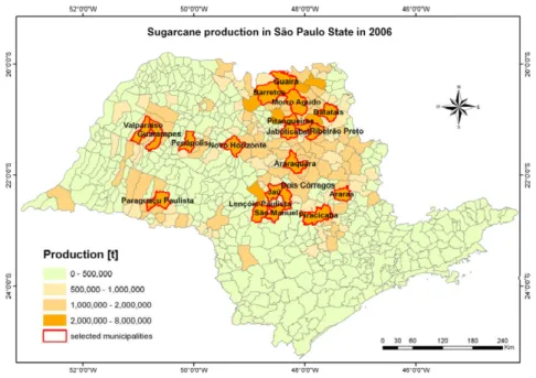
The study was carried out in 20 municipalities in São Paulo State, Brazil, during seven consecutive cropping seasons. All municipalities of São Paulo State were ranked in descending order by sugar cane average yield in 2006 and 20 municipalities of the top were selected. Average municipal yield data for sugarcane were ob-tained from IBGE (2008). The SPOT Vegetation images were made available from 1999, thus, for this reason, the period analyzed was defined between August 1999 and October 2006. Figure 1 shows the spatial distribution of sugarcane production in São Paulo State in 2006 and the selected municipalities.

The SPOT Vegetation offers free low spatial resolu-tion NDVI images (1 km × 1 km pixel) with high tem-poral resolution (daily) (Vegetation, 2007). About 255 im-ages of SPOT Vegetation product S10 (NDVI 10-day

composite) atmospherically and geometrically corrected were used in this study.

Meteorological data, estimated by the European Cen-ter for Medium-range Weather Forecast (ECMWF) global model, interpolated at 0.5 degrees resolution, in the form of 10-daily composite images (geotiff format), are freely available at the Joint Research Centre (JRC, 2007) of the European Commission. The following meteorological vari-ables were selected: Rainfall (in mm, accumulated value for every 10-day period); Global radiation (in Wh/m², ac-cumulated value for every 10-day period); Minimum tem-perature (in °C, mean for every 10-day period); Medium temperature (in °C, mean for every 10-day period); Maxi-mum temperature (in °C, mean for every 10-day period). Both 10-daily NDVI and meteorological data were gath-ered for the period between August 1999 and October 2006. The Hants (Harmonic Analysis of NDVI Time-Se-ries) algorithm was applied to NDVI annual time series in order to eliminate abrupt variations in the 10-day NDVI values usually caused by the presence of clouds. This algorithm, proposed by Roerink et al. (2000), con-siders the NDVI temporal behavior throughout a crop-ping season as harmonic and with low frequency. There-fore, the series was adjusted by eliminating high fre-quency oscillation regarded as ‘noise’. The adjustment was based on the minimum quadratic error. Figure 2 shows, as an example, the adjustment of values origi-nated from a pixel in sugarcane cultivation area.

A Geographical Information System (GIS) was used to select pixels located in sugarcane planted areas from the SPOT Vegetation images. Thematic maps from CANASAT (2007) were used as reference to locate ar-eas planted with sugarcane in each municipality. Then, the NDVI time series profiles were obtained for each selected pixel in all municipalities and cropping seasons. So, an average municipal NDVI time series profile was

calculated. Average municipal NDVI profiles were used in order to adequate the spatial scale of the spectral data with the yield data available. Average municipal ECMWF meteorological data were also used to gener-ate time profiles for each municipality and cropping sea-son. An automatic process for image data extraction was used through an ENVI/IDL computational system based on the study carried out by Esquerdo et al. (2006).

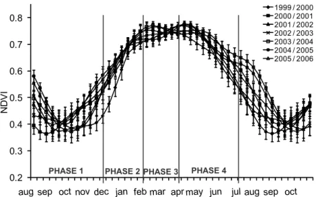
Information about sugarcane physiology was used in order to separate the database in different development phases within the cropping season: establishment, vegeta-tive development and stabilization/senesce, as used by Simões et al. (2005a). The vegetative development was di-vided in two parts: fast growth and slow growth. Thus, the development cycle was divided in 4 phases: establish-ment, fast growth, slow growth and stabilization/senesce. The NDVI is directly related to the crop characteris-tics of the sugarcane (Simões et al., 2005a). For each crop-ping season the average NDVI profile of 20 municipali-ties was calculated to compare different dynamics in plant

Figure 2 – Example of Hants’ algorithm for a pixel in sugarcane cultivation, applied on 10-day SPOT Vegetation images.

0.2 0.3 0.4 0.5 0.6 0.7 0.8

sep oct nov dec jan feb mar apr may jun jul aug sep oct

ND

V

I

original hants

Figure 3 – Average NDVI profiles and standard deviation for each cropping season and definition of four development phases boundaries.

0.2 0.3 0.4 0.5 0.6 0.7 0.8

NDV

I

1999 / 2000 2000 / 2001 2001 / 2002 2002 / 2003 2003 / 2004 2004 / 2005 2005 / 2006

PHASE 1 PHASE 2 PHASE 3 PHASE 4

development among seven cropping seasons. So, the boundaries between phenological stages were defined in crop calendar, based on a general behavior of NDVI data during seven years. The average NDVI profiles and stan-dard deviation among the 20 municipalities, obtained for each cropping season, are shown in Figure 3. Then, NDVI and meteorological data were aggregated by phase, allow-ing for the generation of spectral and meteorological at-tributes for each development phase as well as for the whole cropping season, resulting in 51 attributes for each municipality/cropping season, as shown in Table 1.

To use data mining techniques, such as attribute se-lection and classification by decision tree, the average municipal yield (attribute class) data were discretized in three classes through percentiles. Table 2 shows the three classes of average municipal yield after discretization, as well as their respective lower and up-per limits and number of occurrences.

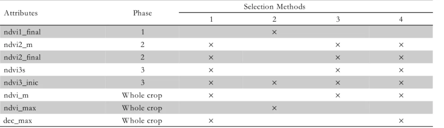
Table 1 – Spectral and meteorological attributes generated for each development phase and for the whole cropping season.

Phase Attribute name Description

PH ASE 1

1 ndvi1_s Sum of N DVI values of phase 1 (accumulated). 2 ndvi1_m Arithmetic mean of N DVI values in phase 1

3 ndvi1_final N DVI value in the last 10-day period of phase 1 (3rd _{10-day period of N ovember)} 4 rain1_s Phase 1 accumulated rainfall

5 grs1_s Phase 1 accumulated global radiation

6 tmin1_m Arithmetic mean of minimum temperatures values of phase 1 7 tmean1_m Arithmetic mean of medium temperatures of phase 1 8 tmax1_m Arithmetic mean of maximum temperatures of phase

PH ASE 2

9 ndvi2s Sum of N DVI values of phase 2 (accumulated)

10 ndvi2_inic N DVI value in the first 10-day period of phase 2 (1st _{10-day period of December)} 11 ndvi2_m Arithmetic mean of N DVI values of phase 2

12 ndvi2_final N DVI value in the last 10-day period of phase 2 (3rd _{10-day period of January )}

13 ndvi2_d Difference between the N DVI values for the last and first 10-day periods of phase 2 N C VI valuesdecêndios da fase 2.

14 rain2s Phase 2 accumulated rainfall 15 grs2s Phase 2 accumulated global radiation

16 tmin2m Arithmetic mean of minimum temperature values of phase 2 17 Tmean2m Arithmetic mean of medium temperatures of phase 2 18 tmax2m Arithmetic mean of maximum temperatures of phase 2

PH ASE 3

19 ndvi3s Sum of N DVI values of phase 3 (accumulated).

20 ndvi3_inic N DVI value in the first 10-day period of phase 3 (1st _{10-day period of February )} 21 ndvi3_m Arithmetic mean of N DVI values in phase 3

22 ndvi3_final N DVI value in the last 10-day period of phase 3 (3rd _{10-day period of March)} 23 ndvi3_d Difference between the N DVI values of the last and first 10-day periods of phase 3 24 rain3s Phase 3 accumulated rainfall

25 grs3s Phase 2 accumulated global radiation

26 tmin3m Arithmetic mean of mean of minimum temperature values in phase 3 27 Tmean3m Arithmetic mean of mean of medium temperatures values in phase 3 28 tmax3m Arithmetic mean of mean of maximum temperatures values in phase 3

PH ASE 4

29 ndvi4s Sum of N DVI values of phase 4 (accumulated)

30 ndvi4_inic N DVI value for the first 10-day period of phase 4 (1st _{10-day period of April)} 31 ndvi4_m Arithmetic mean of N DVI values of phase 4

32 ndvi4_final N DVI value for the last 10-day period of phase 4 (3rd 10-day period of June) 33 ndvi4_d Difference between the N DVI values of the last and first 10-day periods of phase 4 34 rain4s Phase 4 accumulated rainfall

35 grs4s Phase 4 accumulated global radiation

36 tmin4m Arithmetic mean of minimum temperature values of phase 4 37 tmean4m Arithmetic mean of medium temperature values of phase 4 38 tmax4m Arithmetic mean of maximum temperature values of phase 4

W H OLE C RO PPIN G SEASO N

39 ndvis Sum of N DVI values in all phases (accumulated between August and June)

40 ndvi_min Minimum N DVI value occurred for crop

41 dec_min 10-day period of minimum N DVI value, from the 1st _{10-day period of August on} 42 ndvi_m Arithmetic mean of N DVI values for the whole crop

43 ndvi_max Maximum N DVI value occurred for crop

44 dec_max 10-day period of maximum N DVI value, from 1st _{10-day period of August on} 45 ndvi_d Difference between the maximum and minimum N DVI values for crop

46 periodo_mM N umber of 10-day periods (duration) between the occurrence of the minimum and maximum N DVI values for crop

47 rains C rop accumulated rainfall 48 grss C rop accumulated global radiation

To verify the tendency shown in the second classifi-cation correlation analysis were carried out between spectral attributes and average municipal yield using two approaches. The first approach evaluated the average re-sult for each cropping season, considering the 20 munici-palities’ average. The average spectral attribute and the average crop yield among the 20 municipalities were cal-culated for each cropping season. The second approach evaluated the average result for each municipality, con-sidering the average of the seven cropping seasons. The average historical value of the spectral attribute and yield was calculated for each municipality.

Results and Discussion

Table 3 shows the selected attributes for each method. The meteorological attributes were not selected. That could be explained by the fact that the development phases were fixed in the calendar, the duration of each develop-ment phase and the use of cumulative meteorological data. Other reason for absence of selection is related with the method used to discretize the yield. Three classes in per-centiles method may not have been adequate to relate with the numeric meteorological attributes.

Using the ndvi2_m, ndvi2_final, ndvi3_s, ndvi3_inic and ndvi_m attributes, J48 classification algorithm was applied based on decision tree. A threshold was applied defining a minimum number of ten objects. As a train-ing set, a cross validation method with 5 folds was used. From a total of 140 instances, the classifier rated 98 cor-rectly, corresponding to 70% accuracy. Table 4 presents the confusion matrix and accuracy of the performed clas-sification. The diagonal values represent the correctly classified instances.

Balance and coherence of results were observed (Table 4), since there was more confusion between neighboring classes (B-M and M or M and M-A) than between remote classes (B-M and M-A). This confusion may be associated with the discretization method used for the attribute class (average crop yield). The ndvi2_final and ndvi2_m attributes are located on top of the tree, which means an important role in yield clas-sification (Figure 4). They belong to the fast growth phase, gathered between the first 10-day period of De-cember the third 10-day period of January. The behav-ior of these two attributes was coherent, once the higher values of NDVI in the vegetative development phase mean good crop development in the field, favoring

Table 2 – Limits of classes for the average municipal yield and number of occurrences.

C lass Description Lower limit Upper limit Number of occurrences

--- t ha–1 _{--- B-M}

Low-medium 60 73 24 M

Medium 74 85 74 M-A

Medium-high 86 110 42

Original C lassif.

B-M M M-A Accuracy [%]

B-M 15 9 2 62.5

M 6 55 12 74.3

M-A 3 10 28 66.7

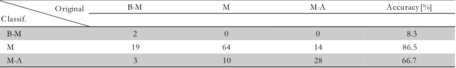
Table 4 – Confusion matrix and classification accuracy for yield rate from ndvi2_m, ndvi2_final, ndvi3_s, ndvi3_inic and ndvi_m attributes.

Table 3 – Selected attributes for each attribute selection method.

Attributes Phase Selection Methods

1 2 3 4

ndvi1_final 1 ×

ndvi2_m 2 × × ×

ndvi2_final 2 × × ×

ndvi3s 3 × × ×

ndvi3_inic 3 × × × ×

ndvi_m W hole crop × × ×

ndvi_max W hole crop ×

higher yield results. Then, a new classification for the same 140 instances using only the ndvi2_final and ndvi2_m attributes was carried out. The classification algorithm continued to be the J48, using a threshold with a minimum number of ten objects, and cross validation method with 5 folds was applied for the training set. The classifier rated 67% of cases correctly, which corre-sponded to 94 out of 140 instances.

There was a significant worsening regarding the clas-sification of yield B-M, whose hit percentage dropped from 62.5 to 8.3 (Tables 4 and 5). Classification of M class yield improved, increasing from 74.3 to 86.5 its ac-curacy percentage. For classification of M-A class, the result did not change.

Figure 5 shows the decision tree for determination of average municipal yield, which was obtained using only the ndvi2_m and ndvi2_final attributes. The analy-sis of both classifications, to determine yield classes M and M-A, showed that it was possible to obtain reason-able results using only the ndvi2_final and ndvi2_m at-tributes; that, though, did not occur with class B-M. Only the ndvi2_final attribute was determinant for the classi-fication of M-A class (Figures 4 and 5). These features were originated from phase 2, which refers to the pe-riod between the beginning of December and the end of January and, therefore, with an anticipation of at least

two months in relation to the beginning of the harvest-ing period. Other factors, besides those considered in this study, influence the official yield figures presented. Special attention should be drawn to the B-M class re-garding low yield indices since, even under favorable field conditions for plant development, low yield may occur if economic factors, for instance, are not favorable. However, for high yield indices to occur, these field con-ditions must be favorable.

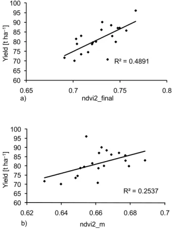
Correlation analyses between the two spectral at-tributes of phase 2 and the average municipal yield were done to evaluate the tendency shown in Figure 5, in which higher values are related to higher yield and vice versa. In the first approach, the option was to evaluate the cropping season average to homogenize differences between standard municipal yields. Figure 6 shows the correlation results between NDVI final/average, NDVI in phase 2 and average yield for each cropping season, considering averages among 20 municipalities. Each dot in the graphs refers to one cropping season. The results from Figure 6 were consistent with the classification pre-sented in Figure 5, i.e., cropping seasons with higher spectral attributes values tended to show higher yields and vice versa.

In the second approach, the goal was to verify whether the municipal yield historical pattern (histori-cal series between 1999 and 2006) could be perceived in the spectral variables. The results presented in Figure 7 also show consistency with the classification result pre-sented in Figure 5, despite the low coefficient of deter-mination. Low coefficient of determination was ex-pected, since the results of the average municipal yield do not depend only on field conditions.

Figure 4 – Decision tree for yield classification using ndvi2_m, ndvi2_final, ndvi3_s, ndvi3_inic and ndvi_m attributes.

Figure 5 – Decision tree for yield classification using ndvi2_final and ndvi2_m attributes.

Original C lassif.

B-M M M-A Accuracy [%]

B-M 2 0 0 8.3

M 19 64 14 86.5

M-A 3 10 28 66.7

Despite the results presented high level of accuracy, they are good indicators for crop monitoring purposes, once they provide a good basis for qualitative assessment of crop yield, as used by institutions such as the Joint Research Center of the European Commission (JRC, 2010), which produces monthly crop monitoring bulle-tins for several regions in the world based on NDVI, sig-naling areas with below average/average/above average conditions for crop development.

Acknowledgements

To the National Council for Scientific and Techno-logical Development (CNPq) for the support received.

References

Boken, V.K. and Shayewich, C.F. 2002. Improving an operational wheat yield model using phenological phase-based Normalized Difference Vegetation Index. International Journal of Remote Sensing 23: 4155-4168.

Canasat. 2007. Mapping sugarcane by earth observation satellites. Avail abl e at: htt p:/ /www.dsr.i npe .br/mapdsr/i ntro.h tm [Accessed Nov. 13, 2007] (in Portuguese).

Co mpanhi a Naci onal d e Abast eci men to [CO NAB]. 2007. Monitoring of the Brazilian S ugar Cane 2007/2008 cropping se aso n, first survey , M ay/2007. Avai lab le at: ht tp:// w w w . c o n a b . g o v . b r / c o n a b w e b / d o w n l o a d / s a f r a / 1_levantamento0708_mai2007.pdf [Accessed Dec. 10, 2007] (in Portuguese).

Esquerdo, J.C.D.M.; Antunes, J.F.G.; Baldwin, D.G.; Emery, W.J.; Zullo Júnior, J. 2006. An automatic system for AVHRR land surface product generation. International Jo urnal of Remote Sensing 27: 3925-3942.

Ferencz, C.; Bognár, P.; Lichtenberger, J.; Hamar, D.; Tarcsai, G.; Timár, G.; Molnár, G.; Pásztor, S.; Steinbach, P.; Székely, B.; Ferencz, O.E.; Ferencz-Árkos, I. 2004. Crop yield estimation by remote sensing. International Journal of Remote Sensing 25: 4113-4149.

Green lan d, D. 2005. Cli mat e variabil ity an d sugarcane yie ld in Louisiana. Journal of Applied Meteorology 44: 1655-1666. I nst it uto Brasi l ei ro d e Geo g raf ia e E st atí sti c a [IBGE]. 2002.

Agri cul tural an d S t oc k R aisin g S urve ys, M e th o do l og i cal Reports Se ries. Available at: http://www.ibge.go v.br/home/ e s t a t i s t i c a / i n d i c a d o r e s / a g r o p e c u a r i a / PesquisasAgropecuarias2002.pdf [Accessed Mar. 07, 2008] (in Portug uese).

In sti tut o Brasile iro de Ge ografi a e Estat íst ica [I BGE ]. 2008. Agg regat es Dat abase . SIDRA - I BGE S ystem for Automatic Re covery . Avai lab le at: htt p:/ /www.sidra.i bge .go v.b r. [Accessed Jun. 29, 2008] (in Portuguese).

Figure 6 – a) Correlation between ndvi final in phase 2 and average yield for each cropping season (considering 20 municipalities). b) Correlation between average ndvi in phase 2 and average yield for each crop (considering 20 municipalities).

Figure 7 – a) Correlation between average final ndvi in phase 2 and average yield for each municipality – historical series between 1999 and 2006; b) Correlation between average ndvi in phase 2 and average yield for each municipality - historical series between 1999 and 2006.

R² = 0.2537

60 65 70 75 80 85 90 95 100

0.62 0.64 0.66 0.68 0.7

Y ield [ t ha –1] ndvi2_m b)

R² = 0.4891

60 65 70 75 80 85 90 95 100

0.65 0.7 0.75 0.8

Y ield [ t ha –1 ] ndvi2_final a)

R² = 0.561

77 78 79 80 81 82 83 84 85

0.7 0.72 0.74 0.76

Y ie ld [ t ha –1 ] ndvi2_final a)

R² = 0.8594

76 77 78 79 80 81 82 83 84 85

0.6 0.62 0.64 0.66 0.68 0.7

Received October 02, 2009 Accepted October 01, 2010 Joint Research Centre [JRC]. 2006. Meteorological Data Simulated

by ECMWF Model. Available at: http://mars.jrc.ec.europa.eu/ mars/About-us/FOODSEC/Data-Distribution [Accessed Apr. 25, 2007].

Joint Research Centre [JRC]. 2006. Bulletins and Publications. Available at: http://mars.jrc.ec.europa.eu/mars/Bulletins-Publications [Accessed Apr. 12, 2010].

Labus, M.P.; Nielsen, G.A.; Lawrence, R.L.; Engel, R. 2002. Wheat yield estimates using multi-temporal NDVI satellite imagery. International Journal of Remote Sensing 23: 4169-4180. Ro eri nk, G.J.; Men ent i, M.; Ve rho ef, W. 2000. Rec onstructi ng

cloudfree NDVI composites using Fourier analysis of time series. International Journal of Remote Sensing 21: 1911-1917. Si mõe s, M.S .; Roc ha, J.V.; Lamparel li, R.A.C. 2005a. Spe ctral

variable s g rowth analysis and yi eld of sugarcan e. Sci ent ia Agricola 62: 199-207.

Si mõe s, M.S .; Roc ha, J.V.; Lamparell i, R.A.C. 2005b . Growth indices and productivity in sugarcane. Scientia Agricola 62: 23-30.

Simões, M.S.; Rocha, J.V.; Lamparelli, R.A.C. 2009. Orbital spectral variables, growth analysis and sugarcane yield. Scientia Agricola 66: 451-461.