Diffusive properties of soft condensed matter systems under external confinement

Diego de Lucena Camarão

Diffusive properties of soft condensed matter systems under

external confinement

Diffuse eigenschappen van zachte gecondenseerde materie

systemen met uitwendige opsluiting

Diego de Lucena Camarão

Diffusive properties of soft condensed matter systems under

external confinement

Doctoral thesis presented to the Department of Physics of Federal University of Ceará as part of the prerequisites to obtain the title of Doctor of Science (D.Sc.)

Federal University of Ceará

Department of Physics

Graduation Program in Physics

Supervisor: Prof. Dr. Wandemberg Paiva Ferreira

Co-supervisor: Prof. Dr. François M. Peeters

Diego de Lucena Camarão. – Fortaleza / CE / Brazil,

2014-141p. : il. (color.) ; 30 cm.

Supervisor: Prof. Dr. Wandemberg Paiva Ferreira Doctoral Thesis – Federal University of Ceará Department of Physics

Graduation Program in Physics, 2014.

1. Soft condensed matter. 2. Colloids. 3. Computer simulation. I. Prof. Dr. Wandemberg Paiva Ferreira. II. Federal University of Ceará. III. Department of Physics. IV. Title

Diego de Lucena Camarão

Diffusive properties of soft condensed matter systems under

external confinement

Doctoral thesis presented to the Department of Physics of Federal University of Ceará as part of the prerequisites to obtain the title of Doctor of Science (D.Sc.)

Approved doctoral thesis. Fortaleza / CE / Brazil, 27/08/2014:

Prof. Dr. Wandemberg Paiva Ferreira

Supervisor (UFC, Brazil)

Prof. Dr. François M. Peeters

Co-supervisor (UAntwerpen, Belgium)

Prof. Dr. Ramón Castañeda-Priego

University of Guanajuato, Mexico

Prof. Dr. Fabrício Q. Potiguar

UFPA, Brazil

Prof. Dr. Gil de Aquino Farias

UFC, Brazil

Prof. Dr. Raimundo N. da Costa Filho

UFC, Brazil

Acknowledgements

I would like to kindly express my full gratitude to my supervisor Prof. Wandemberg Paiva

Fer-reira, for all the support during the development of this thesis. Not less important is my gratitude

towards my co-supervisor Prof. François Peeters for all his insightful comments to improve this

thesis, and specially his endless patience. I would also like to thank Prof. Felipe Munarin, Dr.

Kwinten Nelissen and Dr. Vyacheslav Misko for all the support during the preparation of some

of the works presented in this thesis.

Scientific developments are certainly not a result of individual achievement, therefore

I would like to thank all people involved in my life during all these (almost) four years of my

PhD studies, specially my family and my friends. It would be unfair if I forgot any names, so

I’ll just keep it simple and plain: Thank you very much for all the support throughout these

years.

I would also like to thank all the employees from the Department of Physics of Federal

University of Ceará (UFC) and from the Department of Physics of University of Antwerp (UA).

Last but not least, I would like to thank the Brazilian agencies CAPES and CNPq, and the

Flemish agency FWO, for financial support.

Diego

“The first principle is that you must not fool yourself.

And you are the easiest person to fool.”

Abstract

In this thesis we study the influence of external confinement potentials on the dynamical

prop-erties of soft condensed matter systems. We analyze the diffusive propprop-erties of two specific

systems by means of Langevin and Brownian Dynamics simulations. In Chapter 1, we

intro-duce the subject of soft condensed matter. We show several theoretical and experimental aspects

of these type of systems. We make a brief introduction to the topic of diffusion (Sec.1.5), where

we discuss main aspects of Brownian motion. We introduce the single-file diffusion (SFD)

prob-lem (Sec.1.5.3) and discuss it in the context of soft condensed matter systems, both theoretically

and experimentally. In Chapter 2, we introduce the computational method used in this thesis.

We discuss Molecular Dynamics (MD) and its variants, Langevin and Brownian Dynamics

sim-ulations. We also introduce numerical algorithms used in the following chapters. In Chapters

3, 4and5, we analyze two different systems, namely (i) a system of interacting Yukawa

parti-cles confined in a parabolic quasi-one-dimensional (q1D) channel and (ii) a system of magnetic

colloidal particles under the influence of both a parabolic confinement potential and a periodic

external modulation along the unconfined direction. In the former, we study the transition from

the single-file diffusion (SFD) regime to the two-dimensional (2D) diffusion regime. In the

lat-ter, we study the influence of several parameters that characterizes the system, e.g., the strength

of an external magnetic field and the periodic modulation along the unconfined direction, on its

dynamical properties. Finally, we present the summary of the main findings reported in this

the-sis and we show some open questions as perspectives for future research in the field of diffusion

in soft condensed matter systems.

Resumo

Nesta tese estudamos a influência de potenciais de confinamento externos nas propriedades

dinâmicas de sistemas de matéria condensada mole. Analisamos as propriedades difusivas

de dois sistemas específicos utilizando simulações computacionais (Dinâmica Molecular de

Langevin e Dinâmica Browniana). No Capítulo1, introduzimos o tópico sobre matéria

conden-sada mole. Mostramos vários aspectos teóricos e experimentais neste tipo de sistema. Fazemos

uma breve introdução ao tópico de difusão (Sec.1.5), onde discutimos os principais aspectos do

movimento Browniano. Introduzimos o problema de difusão em linha (SFD, do inglês

single-file diffusion) (Sec.1.5.3) e o discutimos, teorica e experimentalmente, no contexto de sistemas de matéria condensada mole. No Capítulo2, introduzimos os métodos computacionais

utiliza-dos nesta tese. Discutimos os métoutiliza-dos de Dinâmica Molecular e suas variantes, o método de

Dinâmica de Langevin e Dinâmica Browniana. Também introduzimos algoritmos de integração

utilizados nos capítulos posteriores. Nos Caps. 3,4e5, analisamos dois sistemas distintos, (i)

um sistema de partículas de Yukawa confinadas em um canal parabólico quasi-unidimensional

(q1D) e (ii) um sistema de colóides magnéticos sob a influência de um potencial parabólico

e uma modulação periódica externa ao longo da direção não confinada. No primeiro sistema,

estudamos a transição do regime de difusão em linha (SFD) para o regime de difusão normal

(2D). No segundo sistema, estudamos os efeitos de vários parâmetros que caracterizam o

sis-tema (e.g., a magnitude do campo magnético externo e a presença da modulação periódica

externa) em suas propriedades dinâmicas. Finalmente, apresentamos um sumário dos

princi-pais resultados obtidos nesta tese e mostramos algumas questões em aberto como perspectivas

para pesquisas futuras na área de difusão em sistemas de matéria condensada mole.

Samenvatting

In deze thesis werd de invloed van uitwendig aangelegde inperkingspotentialen onderzocht op

de dynamische eigenschappen van zacht gecondenseerde materie systemen. De diffusie

ei-genschappen van twee specifieke systemen werden onderzocht doormiddel van Langevin en

Brownse dynamische simulaties. In Hfst. 1 wordt het onderwerp van zacht gecondenseerde

materie geintroduceerd. Verschillende theoretische en experimentele aspecten van dit type van

systemen worden vermeld. Ook wordt er een korte inleiding gegeven van het onderwerp

diffu-sie (Sec. 1.5), waar de verschillende hoofd aspecten van Brownse beweging worden vermeld.

Het probleem van ‘single file’ diffusie (SFD) (Sec.1.5.3) wordt geintroduceerd en besproken in

de context van zacht gecondenseerde materie systemen, zowel theoretisch als experimenteel. In

Hfst. 2, wordt de computationele methode besproken die in deze thesis werd aangewend. We

bespreken de Moleculaire Dynamica (DM) simulatie methode en de varianten zoals Langevin

and Brownse dynamische simulaties. De numerieke algoritmen die in de volgende hoofstukken

worden aangewend worden geintroduceerd. In de Hfst. 3, 4en5analyzeren we twee

verschil-lende systemen, namelijk: (i) een systeem van interagerende Yukawa deeltjes die opgesloten

zijn in een parabolische kwasi-één-dimensionaal (q1D) kanaal, en (ii) een systeem van

mag-netisch colloidale deeltjes onder de invloed van een parabolische inperkingspotentiaal en een

periodisch externe modulatie langs de vrije richting. In het eerste systeem bestuderen we de

overgang van het ‘single-file’ diffusie regime naar het twee-dimensionaal diffusie regime. We

bestuderen de invloed van de verschillende parameters die het systeem karakteriseren, bijv. de

sterkte van het uitwendig magneetveld en de aanwezigheid van een periodische modulatie langs

de vrije richting op de dynamische eigenschappen. Eindelijk, presenteren we de overzicht van

de thesis en we vermelden een aantal open vragen die interessant zijn voor toekomst onderzoek

in het gebied van diffusie van zacht gecondenseerde materie systemen.

List of Figures

Figure 1 – Examples of soft condensed matter systems. Top panel: (left) Paints, and

(right) powder soap. Bottom panel: (left) A colloidal gel dispersion, and

(right) glue. . . 30

Figure 2 – Schematic representation of polystyrene colloidal particles of radius R=1.4

µm dispersed in heavy water (D2O) and confined by external laser beams.

Taken from Ref. (10). . . 31

Figure 3 – (a) Schematic representation of a Penning trap, where charged particles are

confined by using electric and magnetic fields. (b) Sketch of the experiment

used to confine the particles and (c) image of the actual device used in the

experiments of Ref. (16). . . 32

Figure 4 – (a) Schematic representation of the electric double layer, which consists of

the positively charged cloud of counter ions around the colloidal particle

and the negatively charged surface (total charge Z) of the colloidal particle.

(b) Two colloidal particles interact with each other through a repulsive

inter-particle interaction potential which is screened by the cloud of counter ions.

Taken from Ref. (20). . . 33

Figure 5 – A 2D system of N=230 electrons confined by a parabolic trap and

interact-ing through a repulsive potential tend to form a Wigner crystal in the

cen-ter. However, some defects can appear due to the competition between the

confinement potential (trap) and the repulsion between the particles. Also,

particles in the borders tend to be accommodated in a distorted triangular

lattice. Taken from Ref. (26). . . 35

Figure 6 – A series of Wigner crystal structures showing the arrangement of electrons

in a circular island from an occupation number of N =3 to N=100. The

electrons form ring structures as more electrons are added. For large N,

a triangular Wigner lattice forms in the center, while the outer electrons

remain in rings. Taken from Ref. (29), illustration by Alan Stonebraker.. . . 36

Figure 7 – Representation of a dusty plasma. The free positive ions in the plasma

ad-here to the surface of the dust particles creating a strong electrostatic

repul-sive interaction between these particles. Taken and adapted from Ref. (30). . 37

Figure 8 – Trajectory of a particle executing a Brownian movement. Note that the

movement is very irregular and experiments by Robert Brown showed that

the movement is most active in less viscous liquids and less active for lower

channels with the particles (black dots) inside. Taken from Ref. (41). . . 41

Figure 10 – Pictorial representation of periodic boundary conditions (PBC) for a 2D

sys-tem. In the center, there is the main computational unit cell, and the identical

copies around it. From Ref. (71) . . . 50

Figure 11 – (a) In the center there is the reference particle (dark circle). The circles

around it represents other particles in the system. A centered ring is drawn

as reference and it has radius r and width dr. (b) As an example, we show

the typical radial distribution function for a Lennard–Jones system in the

liquid phase. Taken from Ref. (74). . . 53

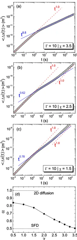
Figure 12 – (a)-(c) Log-log plot of the mean square displacement (MSD)_h∆x2(t)_ias a function of time for different values of χ. Different diffusion regimes can

be distinguished: normal diffusion regime (α =1.0) and intermediate

sub-diffusive regime (ITR,α <1.0). Note that for the case ofχ = 1.5, there is a

normal diffusion regime (i.e. α =1.0) after the ITR. The dashed and solid

lines in (a)-(c) are a guide to the eye. Panel (d) shows the dependence of

the slope (α) of the MSD curves (in the ITR, characterized by an apparent

power-law;_h∆x2(t)_i∝tα) on the confinement strengthχ. . . 67 Figure 13 – (a)-(c) Log-log plot of the mean square displacement (MSD)_h∆x2(t)_ias a

function of time for different values of Rw. Different diffusion regimes can

be distinguished: normal diffusion regime (α =1.0) and intermediate

sub-diffusive regime (ITR,α<1.0). Note that for the case of Rw= 0.60, there is

a normal diffusion regime (i.e. α =1.0) after the ITR. The dashed and solid

lines in (a)-(c) are a guide to the eye. Panel (d) shows the dependence of

the slope (α) of the MSD curves (in the ITR, characterized by an apparent

power-law;_h∆x2(t)_i∝tα) on the confinement parameter Rw. . . 68

Figure 14 – (a)-(b) Exponent α as a function of time, calculated from Eq. (3.15) for

different values of the confinement parametersχ and Rw, respectively. . . . 69

Figure 15 – (a) Number of crossing events C(t)as a function of time for N =400

par-ticles, for χ=1.5 (black open circles) andχ=3.5 (green open diamonds).

The solid red line is a linear fit to C(t). Panels (b) and (c) show the rate

of the crossing eventsωc as a function of the confinement potential

param-eters (χ and Rw). The insets in the panels (b) and (c) show the derivatives,

dωc(χ)/dχ and dωc(Rw)/dRw, correspondingly.. . . 72

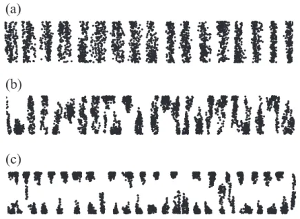
Figure 16 – For the hard-wall confinement case, we show typical trajectories of particles

(i.e. 106 MD simulation steps) confined by the channel of width (a) Rw=

Figure 17 – Probability distribution of the particle density P(y)along the y-direction are

shown for (a) different values ofχ (parabolic 1D confinement) and (b) four

different values of the width Rwof the channel (hard-wall confinement). . . 74

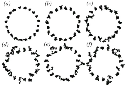
Figure 18 – Trajectories of N=20 particles diffusing in a ring of radius rch=9 mm for

106consequent time steps for different values of γ. γ=1 (a), 2 (b), 3 (c), 5

(d), 7 (e), 9 (f). . . 76

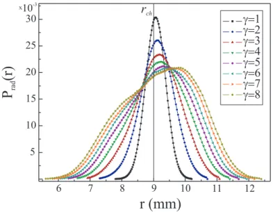
Figure 19 – The distribution of the probability density of particles Prad(r)in a circular

channel of radius rch =9 mm along the radial direction r. The different

curves correspond to various γ. Increasingγ the width of the distribution

Prad(r)increases due to a weakening of the confinement. . . 77

Figure 20 – Spatial distribution of the potential Vint(r,φ)created by a particle (red (grey)

circle) and the qualitative distribution of the probability density of particles

in circular channel Prad(r)(green (light grey) line) along the radial direction

r. The function∆r determines an approximate radial distance between parti-cles when the potential barrier Ubar becomes “permeable” for given

temper-ature T . The function∆rsw characterizes a width of the distribution Prad(r)

at this temperature T . . . . 77

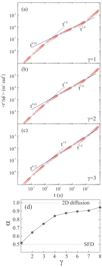
Figure 21 – (a)–(c): Log-log plot of the mean square displacement (MSD) _h∆φ2_i as a function of time for different values of the “effective” temperature γ = (a)

1, (b) 2, and (c) 3. Here (Nens=100,Npar =20). (d) The diffusion

expo-nent α as a function of γ. Increase of the “effective” temperature γ leads

to the gradual transformation of the single-file regime of diffusion into the

diffusion regime of free particles. . . 80

Figure 22 – Log-log plot of the MSD _h∆x2(t)_i(a) and corrected MSD _h∆x2(t)_icorr (b)

as a function of time for different values of the probability P of bypassing.

Averaging was done over Nsim=1000 ensembles. . . 82

Figure 23 – Schematic representation of the system. The particles have diameterσ and

dipole moment µµµ_i, which forms an angle θi with respect to the x-axis. An

in-plane external magnetic field B is applied with magnitude B andφ is the

angle between B and the x-axis. . . . 87

Figure 24 – Potential energy, as defined by Eqs. (4.4)-(4.5), per particle as a function of

time t for B=100, µ =2.0. In the inset we show the same, but for B=2.

In both cases, the number of particles in the computational unit cell was

N=300 and all the other parameters are given in Sec. 4.2.2. . . 89

Figure 25 – Dipole-dipole interaction potential V_dip(r) [Eq. (4.9)] as a function of the

function of the time t for B=100 and (a)φ =90 , (b)φ =70 , (c)φ =50

and (d) φ =0o. The dashed orange lines are a guide to the eye and the crossover time tcfor each case is indicated by the vertical arrow. . . 93

Figure 27 – (a) Mobility Fb in region (II) as a function of φ and (b) crossover time tc

between the STND regime and the sub-diffusive regime as a function of

φ. The solid lines are a guide to the eye. The dashed vertical line in (b) divides regions with (II) and without (I) an attractive part in the inter-particle

interaction potential. . . 94

Figure 28 – (a) Minimum inter-particle distance d between neighboring particles for

B=100 and T =1.0 as a function of the orientationφ of the external field.

(b) Exponent of diffusion (α) as a function of the orientation φ of the

ex-ternal magnetic field. Note that d decreases with decreasingφ in the region

0o<φ .55o, which is the same region where we found the increase of the diffusion mechanism [cf. panel (b)]. The solid lines are a guide to the eye. . 95

Figure 29 – Typical snapshots of the system after 106 simulation time steps for (a)φ =

90oand (b)φ =30o. Other parameters are B=100 and T =1.0. . . 96 Figure 30 – Mean-square displacement of the system [open black circles, W(t)] and

mean square displacement of individual particles [gray triangles, Wj(t)] as a

function of the time t for two different values ofφ =(a) 90oand (b) 0o. The dashed orange lines are a guide to the eye. Other parameters are B=100

and T =1.0. . . 97

Figure 31 – Log-log plot of the mean square displacement (solid black curves) W(t)as a

function of the time t for B=0.1 and (a)φ =90o, (b)φ =70o, (c)φ =50o and (d) φ =0o. The dashed orange lines are a guide to the eye and the crossover time tcfor each case is indicated by the vertical arrow. . . 98

Figure 32 – Typical snapshots of the system after 106 simulation time steps for (a)φ =

90oand (b)φ =30o. Other parameters are B=0.1 and T =1.0. . . 98 Figure 33 – Log-log plot of the mean square displacement (solid black curves) W(t)as

a function of the time t forφ =90oand (a) B=10, (b) B=2, (c) B=1 and (d) B=0.1. The dashed orange lines are a guide to the eye. . . 99

Figure 34 – Exponent of diffusionα (in the ITR regime) as a function of the strength B

of the external magnetic field forφ =90o. The solid line is a guide to the eye. 99 Figure 35 – Log-log plot of the mean square angular displacement Wrot(t)as a function

of the time t forφ =90oand B=10, B=2, B=1 and B=0.1. The dotted orange horizontal lines correpond to the saturation values of Wrot(t). . . 100

Figure 36 – Effective self-diffusion coefficient Deff/D0 of a single-particle in one

di-mension in the presence of a thermal bath and a periodic potential V(x′) =

Figure 37 – Snapshot of the configuration of the system for V0/kBT =2.0. The particles

are represented by yellow circles where the black arrows indicate the

direc-tion of the dipoles. The contour plot of the potential Vmod(x) +Vconf(y) is

also shown. The linear density isρ =0.5σ−1 and the transversal

confine-ment strength isω =1.0p2kBT/mσ2. . . 108

Figure 38 – Log-log plot of the mean square displacement in the x direction Wx(t) as

a function of time t for different values of the ratio V0/kBT . The yellow

dotted line is a guide to the eye. The open diamonds indicate approximately

the time scale (tN) where the normal diffusive regime, i.e. Wx(t) ∝t, is

recovered. The transversal confinement strength is ω = 1.0p2kBT/mσ2

and the linear density isρ=0.5σ−1. . . 109

Figure 39 – Long-time self-diffusion coefficient Ds/D0as a function of the ratio V0/kBT ,

for different linear densitiesρ. The effective self-diffusion coefficient Deff/D0

[Eq. (5.2)] as a function of V0/kBT for a single particle is also shown (solid

red curve) for comparison. The inset shows the ratio R=Ds/Deffas a

func-tion of V0/kBT for the caseρ =0.5σ−1. . . 110

Figure 40 – (a) Log-log plot of the mean square displacement in the x direction, Wx(t),

as a function of time t for different values of the ratio V0/kBT . The yellow

dotted line is a guide to the eye. The transversal confinement strength is

ω =10.0p2kBT/mσ2and the linear density isρ =0.5σ−1. Vertical black

arrows indicate the relaxation time tc. Inset: Single-file diffusion mobility F,

obtained from the relation (5.16), as a function of V0/kBT . (b) Snapshot of

the configuration of particles (black dots) for V0/kBT=1.0. The modulation

Vmod(x)is plotted as the solid red curve. . . 111

Figure 41 – The same as Fig. 37 but now for V0/kBT =4.0. Linear density is (a) ρ =

0.25σ−1, and (b)ρ=0.75σ−1. For both cases, the transversal confinement

strength isω =1.0p2kBT/mσ2and the commensurability factor is p=1. . 112

Figure 42 – The same as Fig. 38 but now for density (a) ρ =0.25σ−1, and (b) ρ =

0.75σ−1. The transversal confinement strength isω=1.0p2kBT/mσ2and

the commensurability factor is p=1. . . 113

Figure 43 – (a)-(c) Log-log plot of the mean square displacement in the x direction Wx(t),

as a function of time t for different values of the ratio V0/kBT . The yellow

dotted line has a slope of 1 and is a guide to the eye. The transversal

confine-ment strength isω =1.0p2kBT/mσ2and the linear density isρ=0.5σ−1.

Color code is the same as in Fig. 42. (d) Long-time self-diffusion coefficient,

Ds, as a function of V0/kBT for different values of the commensurability

mensurability factor p=(a) 1/2, (b) 1 and (c) 3/2. For all cases, the strenght

of the x direction modulation is V0/kBT =2.0. Note that L changes

accord-ing to the value of p. . . . 115

Figure 45 – (a) Snapshot of the configuration of particles (black dots) for V0/kBT =3.0.

The modulation Vmod(x) is plotted as the solid red curve. (b), (c) Log-log

plot of the MSD as a function of time t in the parallel and transversal

di-rection, respectively, for different values of V0/kBT . The dotted yellow line

has a slope of 1, the magenta dotted-dashed line has a slope of 0.35 and

both are guide to the eye. The open diamonds in (b) [(c)] indicate

approxi-mately the time scale (tN) where the normal diffusive regime [sub-diffusive

regime] appears. (d) Parallel self-diffusion coefficient D_||and (e) anomalous

transversal diffusion coefficient Ktrans, both as a function of V0/kBT .

Param-eters of the simulation are p=2,ρ=1.0σ−1andω =1.0p2kBT/mσ2. . . 118

Figure 46 – Log-log plot of the transversal MSD Wy(t) as a function of time t, for

dif-ferent values of V0/kBT . The magenta dotted-dashed line has a slope of 0.5

and is a guide to the eye. Inset: snapshot of the configuration of particles

(black dots) for V0/kBT =4.0. The modulation Vmod(x) is plotted as the

solid red curve. Parameters of the simulation are p=4, ρ =2.0σ−1 and

Contents

I Literature review

27

1 Soft condensed matter . . . . 29

1.1 General considerations . . . 29

1.2 Colloidal dispersions . . . 30

1.3 Pair interaction between colloidal particles . . . 32

1.3.1 van der Waals forces . . . 32

1.3.2 Debye-Hückel inter-particle interaction potential . . . 33

1.4 Structural and dynamical properties of colloidal dispersions . . . 34

1.4.1 Wigner crystals . . . 34

1.5 Diffusion and Brownian motion. . . 35

1.5.1 Diffusion equation . . . 35

1.5.2 Brownian motion . . . 38

1.5.3 Single-file diffusion (SFD) . . . 40

II Methods

43

2 Computer simulation . . . . 45

2.1 Introduction . . . 45

2.2 Molecular Dynamics (MD) . . . 46

2.2.1 Description of the MD method . . . 47

2.2.2 Numerical integration algorithms . . . 48

2.2.2.1 The Verlet algorithm . . . 48

2.2.2.2 The leapfrog algorithm . . . 49

2.2.3 Periodic boundary conditions (PBC) . . . 50

2.2.4 Calculation of physical properties . . . 51

2.2.4.1 Radial distribution function (RDF) . . . 52

2.2.5 Relation between MD and statistical mechanics . . . 54

2.3 Langevin Dynamics (LD) . . . 54

2.3.1 Brownian Dynamics (BD) . . . 55

2.3.2 Numerical integration of stochastic differential equations . . . 56

IIIResults

59

3 Single-file to two-dimensional diffusion . . . . 61

3.1 Introduction . . . 61

3.2 Model system and numerical approach . . . 63

3.3.2 “Long-time” behavior of the MSD curves and crossing events C(t) . . . 70

3.3.3 Distribution of particles along the y-direction . . . 71

3.4 Diffusion in a circular channel . . . 73

3.4.1 Breakdown of SFD . . . 76

3.4.2 Diffusion regimes . . . 78

3.5 Discrete site model: The long-time limit . . . 79

3.6 Concluding remarks . . . 83

4 Tunable diffusion of magnetic particles . . . . 85

4.1 Introduction . . . 85

4.2 Model and Numerical Methods . . . 87

4.2.1 Model System . . . 87

4.2.2 Numerical Methods . . . 88

4.3 Interaction potential between two dipoles . . . 90

4.4 Influence of a strong external magnetic field on diffusion . . . 91

4.4.1 Region (I): 55o.φ ≤90o . . . 92 4.4.2 Region (II): 0o_≤φ .55o. . . 92 4.5 Exponent of diffusion (α) in the intermediate (ITR) sub-diffusive regime . . . . 93

4.6 Weak magnetic fields . . . 96

4.7 Influence of the strength of the magnetic field . . . 97

4.8 Concluding remarks . . . 100

5 Single-file and normal diffusion of magnetic colloids . . . 103

5.1 Introduction . . . 103

5.2 Single-particle in an external periodic potential . . . 104

5.3 Interacting magnetic dipoles . . . 105

5.4 Normal and single-file diffusion for fixed linear density . . . 107

5.4.1 Caseω =1.0p2kBT/mσ2 . . . 107

5.4.2 Caseω =10.0p2kBT/mσ2 . . . 108

5.5 Effect of linear density on diffusion. . . 110

5.6 Effect of commensurability factor . . . 111

5.7 Anisotropic diffusion and transversal sub-diffusion . . . 114

5.7.1 Two particles per potential well. . . 114

5.7.2 Four particles per potential well . . . 116

5.8 Concluding remarks . . . 117

Summary . . . 121

Appendix

135

A.1 Interaction torque and external magnetic field torque . . . 137

Annex

139

ANNEX A Annex . . . 141

A.1 List of publications related with this thesis . . . 141

Part I

29

1 Soft condensed matter

In this chapter we introduce the topic of Soft Condensed Matter. We define colloidal

disper-sions and we give motivation for using these particles as model systems for testing theoretical

predictions of statistical physics. Many of the ideas presented here can be found in the

follow-ing much more specialized textbooks: “Soft condensed matter” by R. A. L. Jones and “Soft

matter physics” by Masao Doi.

1.1

General considerations

Condensed matter physics is a discipline in the field of Physical Sciences which studies the

physical properties of condensed phases of matter (1). It is mainly concerned in addressing

problems related to liquid and solid systems, but it also deals with different condensed phases

as, for instance, the Bose-Einstein condensate (BEC) in cold atomic systems (2) and the

super-conducting phase (3) found in low temperature materials.

However, there is a variety of materials found in nature which do not fall into the

cat-egory of either simple liquids or crystalline solids. For instance, glues, paints, soaps, and

col-loidal gels (Fig.1) are examples of these type of materials. They are usually referred to as soft

condensed matter systems (4) or soft matter, for short. These systems are formed of colloidal particles (solute) which are dispersed in another liquid (solvent). For example, fat and proteins

in milk are types of colloidal dispersions (_∼0.1µm of diameter) embedded in water.

All of these soft matter systems share some common characteristics. For example, the

characteristic length scale of colloidal dispersions is in an intermediate regime between the

atomic scale and the macroscopic scale. It is therefore usual to refer to colloidal dispersions

as a class of mesoscopic systems. The diameter of the colloidal particles ranges between 10

nm and 10µm. Another feature is that the common physical properties of these materials (e.g.,

self-assembly and non-linear response to external perturbations) are related to the fact that the

energy scales involved are of the order of the thermal energy, kBT . This means that quantum effects do not play an important role in the properties of soft matter systems, which make them

strong candidates for testing theoretical models in statistical physics using relatively simple

Figure 1 – Examples of soft condensed matter systems. Top panel: (left) Paints, and (right) powder soap. Bottom panel: (left) A colloidal gel dispersion, and (right) glue.

1.2

Colloidal dispersions

A colloidal particle of diameter_∼1µm at room temperature T =300 K in water has a

charac-teristic relaxation time1τs∼1 s. Therefore, the dynamics of this particle can be time resolved

using an experimental technique called video microscopy, which consists in recording the

parti-cle’s trajectory to extract useful information not only about the dynamics of the particle itself,

but also about the fluid properties in which it is embedded in.

On the other hand, in atomic systems, where particles have a diameter of a few angstroms,

the characteristic relaxation time is of the order ofτs ∼10−9 s, which is too short for

time-resolved experiments with atomic resolution. In principle it is also possible to study atomic

systems by means of atomic force microscopy (AFM), but colloidal dispersions are usually

more simple and flexible. The main experimental tools to study the static and dynamical

proper-ties of colloidal suspensions are static and dynamic light scattering (SLS and DLS, respectively)

(5,6).

Furthermore, mesoscopic systems can be much more easily tuned in experiments. The

interaction of colloids with external fields and the inter-particle interaction potential between

1.2. Colloidal dispersions 31

pairs of colloids are customizable in order to allow the study of different basic physical problems

in statistical physics. For instance, colloidal crystals show similar diffraction patterns (7) as

X-ray diffraction in atomic systems. One could also, for example, use colloidal crystals as model

systems to study kinetics of crystallization (8, 9), a much more difficult task to achieve using

atomic systems.

Figure 2 – Schematic representation of polystyrene colloidal particles of radius R= 1.4 µm dispersed in heavy water (D2O) and confined by external laser beams. Taken from Ref. (10).

As stated above, one major advantage of using colloidal particles as model systems

to study theoretical predictions of statistical physics is the possibility to tune inter-particle

in-teraction potentials. For instance, colloids can interact through a screened Coulomb potential

(commonly known as the Yukawa potential) or through a dipole-dipole potential, just to cite a

few. In the first case, the strength of interaction between colloids can be tuned by changing the

salt concentration of the solution in which the particles are moving in. In the second case, the

magnetic interaction (dipole-dipole) can be adjusted by introducing an external magnetic field

which induces a magnetic dipole moment inside the colloidal particles. The strength of this

interaction is then proportional to the magnitude of the external magnetic field. The Yukawa

po-tential has an exponential decay form, V(r)∝exp(₋r/λD)/r and the dipole-dipole interaction

has a 1/r3dependence, where r is the center-to-center distance between a pair of colloids and λDis the so-called Debye screening length (11).

Besides the tuning of the inter-particle interaction potential by adjusting external

param-eters, it is also possible to experimentally control the interaction of colloidal particles with

exter-nal fields (cf. Fig.2). For instance, colloidal dispersions can be placed on the top of modulated

(either periodic or random) substrates which are created by using, e.g., light fields (10,12,13).

Furthermore, several types of external potential shapes can be also realized experimentally by

using topographic patterns (14,15).

One of the devices used to experimentally trap colloidal charged particles is called a

Penning trap, where both an electric and a magnetic field are used to confined the particles.

This device usually has a cylindrical symmetry (Fig.3) and batteries are placed on the tips of

temperature of the system to very low values, where liquid and crystal phases are found.

Figure 3 – (a) Schematic representation of a Penning trap, where charged particles are confined by using electric and magnetic fields. (b) Sketch of the experiment used to confine the particles and (c) image of the actual device used in the experiments of Ref. (16).

1.3

Pair interaction between colloidal particles

1.3.1

van der Waals forces

In general, colloidal particles interact with each other through van der Waals forces. In the

case of the spherical particles, the van der Waals potential is given by the analytical expression

(17,18)

V(ri j) =₋C

" 2R2

r2_{i j−}4R2+ 2R2

r2_{i j} +ln 1+

4R2

r2_{i j}

!#

, (1.1)

where ri j is the center-to-center distance between a pair of particles i and j, R=σ/2 is the

radius of each particle, and C is a constant that depends on the type of colloidal particle and

the medium where it is embedded2. Note that the negative sign in Eq. (1.1) indicates that this

interaction is strongly attractive and therefore colloidal particles tend to stick together, which

is known as the coagulation effect. In order to study different kind of effects other than the

coagulation, it is of course desirable to have stabilized colloidal suspensions. This is mainly

achieved by introducing repulsive interaction between the particles, which can be done, e.g., by

electrostatic stabilization techniques (19).

1.3. Pair interaction between colloidal particles 33

1.3.2

Debye-Hückel inter-particle interaction potential

The surface of a colloidal particle is covered by molecules which are electrically neutral.

How-ever, when a colloidal particle is dispersed in water (for instance) the positive charged counter

ions of the molecules are dissolved due to water molecule polarization (20). Therefore, the

surface of the particle is negatively charged and the entropy tends to spread the ions over the

whole volume. When equilibrium is reached, the balance between energy and entropy creates

an electric double layer (21). This layer consists of the positively charged cloud of counter

ions around the colloidal particle and the negatively charged surface of the colloidal particle

itself. Therefore, the cloud of counter ions around the particle is responsible for screening the

interaction between colloidal particles.

Figure 4 – (a) Schematic representation of the electric double layer, which consists of the posi-tively charged cloud of counter ions around the colloidal particle and the negaposi-tively charged surface (total charge Z) of the colloidal particle. (b) Two colloidal particles interact with each other through a repulsive inter-particle interaction potential which is screened by the cloud of counter ions. Taken from Ref. (20).

In order to calculate the inter-particle interaction potential for this case, the

Poisson-Boltzmann (PB) equation

ε0εW∇2φ(r)∝exp

−zie_kφ(r)

BT

, (1.2)

can be solved analytically (11) in the first-order approximation case (i.e., by linearization of the

PB equation). By doing so, one gets the potentialφ(r)created by a colloidal particle at a point

r in space as

φ(r) = Ze 4πε0εW

exp(σ/2λD) (1+σ/2λD)

exp(₋r/λD)

r , (1.3)

where Z is the total charge (in units of the elementary charge e) on the surface of the colloidal

particle,ε0andεW are the permittivity of vacuum and water, respectively. The Debye screening

length is given by λ_D−1=pε0εWkBT/s with s=∑i(ez2i)ci (zi and ci are the valence and the bulk concentration of the counter ions of type i, respectively). Linear superposition of Eq. (1.3)

leads to the well-known Debye-Hückel (22) inter-particle interaction potential

V(ri j) =

(Ze)2 4πε0εW

exp(σ/2λD) (1+σ/2λD)

2

exp(₋ri j/λD)

ri j

for a pair of colloidal particles i and j separated by a distance ri j. Note that the screening effect

is directly related to the concentration of ions present in the sample, i.e.,λ_D−1∝1/√s. Therefore,

it is possible to experimentally tune the inter-particle interaction potential by adjusting the salt

(ions) concentration of the sample, as previously stated.

Note that, as opposed to the potential of Eq. (1.1), the Debye-Hückel potential is

pos-itive, which means the interaction between particles is repulsive. Consequently, experimental

techniques such as the electrostatic stabilization are mainly based on the adjustment of the salt

concentration of the samples. These adjustments prevent particles agglomeration and allows the

creation of well-defined 2D and 3D lattices of colloidal suspensions, e.g., nanocrystals (23,24).

1.4

Structural and dynamical properties of colloidal dispersions

1.4.1

Wigner crystals

In 1934, physicist Eugene Wigner predicted that a gas of electrons could present a phase

transi-tion from a liquid phase to a solid (crystalline) structure (25). This solid phase is now usually

called a Wigner crystal. The main physical mechanism behind this effect is that for a certain

value below a critical density (n<nc), the potential energy of the electrons dominates over the kinetic energy. Therefore, the spatial arrangement of the electrons becomes very important. In

3D, the electrons form a body-centered cubic (bcc) structure. In 2D, they form a triangular

lattice (Fig.5) and in 1D, the electrons become evenly spaced.

The first experimental observation of the Wigner crystallization of electrons was

re-ported by Grimes and Adams (27) in 1979. They found that, under certain circumstances,

electrons deposited on a 2D substrate of liquid helium would arrange themselves in a triangular

lattice, just like predicted by Wigner.

More recently, in 2009, an experimental and numerical study (28) also reported the

formation of Wigner crystal structures using trapped electrons on the surface of liquid helium.

Even more, by experimentally manipulating electrons one by one, the authors were able to

calculate the energy spectrum to add (or to extract) one electron from the trap with occupation

number N. Depending on N, the system of electrons would arrange itself into ring structures.

Previously, in 1994, Bedanov and Peeters (26) showed a theoretical prediction of the formation

of these ring structures (Fig.6) by means of numerical and analytical calculations.

Nowadays, Wigner crystals are also referred to as crystal phases found in non-electronic

systems (e.g., soft condensed matter systems) at low density regimes. For instance, these phases

have been observed experimentally in dusty plasmas (31). In this experiment, dust particles

dispersed in a weakly ionized argon plasma acquire a negative charge (due to the ions present

1.5. Diffusion and Brownian motion 35

Figure 5 – A 2D system of N =230 electrons confined by a parabolic trap and interacting through a repulsive potential tend to form a Wigner crystal in the center. However, some defects can appear due to the competition between the confinement potential (trap) and the repulsion between the particles. Also, particles in the borders tend to be accommodated in a distorted triangular lattice. Taken from Ref. (26).

particles in water (Sec.1.3.2), the interaction between dust particles is also screened by a double

electric layer. Since the inter-particle interaction potential between these particles is similar to

the one presented in Eq. (1.4), there has been a large number of theoretical and experimental

investigations about the Wigner crystallization phenomenon using soft condensed matter as

model systems.

1.5

Diffusion and Brownian motion

1.5.1

Diffusion equation

Diffusive processes occur frequently in nature and they are directly related to the transport of

any given physical quantity in space and time. For instance, the transport of molecules in a fluid

(molecular diffusion), the heat conduction in a metal bar (heat diffusion) and the movement of a

suspended particle in a viscous fluid (Brownian motion) are a few examples of known diffusive

processes.

One of the first mathematical description of a diffusion phenomenon was due to the

French mathematician Joseph Fourier, in his Théorie analytique de la chaleur (The Analytic

Theory of Heat) published in 1822. He studied the heat conduction through a metal bar and

Figure 6 – A series of Wigner crystal structures showing the arrangement of electrons in a cir-cular island from an occupation number of N =3 to N =100. The electrons form ring structures as more electrons are added. For large N, a triangular Wigner lattice forms in the center, while the outer electrons remain in rings. Taken from Ref. (29), illustration by Alan Stonebraker.

equation of the form

∂

∂tu(x,t) =DT

∂2

∂x2u(x,t), (1.5)

where DT is known is as the thermal diffusion coefficient and it is a material-specific quantity.

In 1855, German physician Adolf Fick published his work on particle diffusion and

established what is known today as the Fick’s laws of diffusion. The first Fick’s law states that

the flux of molecules always goes from regions in space of high concentration of particles to

regions of lower concentration, across a gradient of concentration. In mathematical terms, this

law is written as

jjj=₋D(c)∇∇∇c(rrr,t), (1.6)

where jjj is flux (amount of matter per unit area per unit time), D(c)is the diffusion coefficient which may depend on the concentration profile c(rrr,t). Note that the negative sign in Eq. (1.6) comes from the postulate that the flux of molecules goes from the regions of higher to lower

1.5. Diffusion and Brownian motion 37 ûckel ûckel elétrons elétrons+ -+ + + + + + + - -+

-Plasma

Figure 7 – Representation of a dusty plasma. The free positive ions in the plasma adhere to the surface of the dust particles creating a strong electrostatic repulsive interaction between these particles. Taken and adapted from Ref. (30).

∂

∂tc(rrr,t) +∇∇∇· jjj=0, (1.7)

is valid (there are no sinks or sources, i.e., there is no effective creation or destruction of matter),

the combination of Eqs. (1.6) and (1.7) leads to a similar diffusion equation as obtained by

Fourier

∂

∂tc(rrr,t) =∇∇∇·(D(c)∇∇∇c(rrr,t)). (1.8)

Note that if the diffusion constant is independent of the concentration profile c(rrr,t), Eq. (1.8) reduces to

∂

∂tc(rrr,t) =D∇

2

c(rrr,t), (1.9)

which is similar to the heat diffusion equation and also usually called the second Fick’s law.

A solution to Eq. (1.9), considering an initial condition c(rrr,0) =δ(rrr₋rrr0) (where rrr0 is the initial position of the concentration of particles) and assuming isotropy of space, is given by a

Gaussian propagator (33)

c(rrr,t) = 1

h(t)exp

−|rrr−rrr0|

2

m(t)

, (1.10)

where3 h(t)∝√t and m(t)∝t.

From the distribution c(rrr,t) it is possible to calculate its moments. The first two mo-ments are the commonly studied ones, i.e., the average displacement

hr_i=

Z _∞

−∞r c(rrr,t)dV, (1.11)

and the mean square displacement (MSD)

hr2_i=

Z _∞

−∞r

2

c(rrr,t)dV. (1.12)

These quantities are important because they can be obtained through experiments. Furthermore,

they are directly related to macroscopic quantities, such as temperature and viscosity, as we will

show in the following.

1.5.2

Brownian motion

The random movement of suspended particles on a fluid was first observed by Scottish botanist

Robert Brown in his work A Brief Account of Microscopical Observations (34) published in

1828, where he reported the irregular motion of pollen grains in water. Brown was intrigued by

the phenomenon but could not explain it in terms of any previously known theory at the time.

Much longer after Brown’s reports, in 1888, the French physicist Louis-Georges Gouy

made some important remarks about these random movements. Among these remarks, we cite a

few: (i) The motion is extremely irregular (Fig.8), the trajectory seems to be not differentiable,

and the motion never ceases; (ii) the motion is most active4 in less viscous liquids; (iii) the

motion is most active at higher temperatures.

Figure 8 – Trajectory of a particle executing a Brownian movement. Note that the movement is very irregular and experiments by Robert Brown showed that the movement is most active in less viscous liquids and less active for lower temperatures.

These observations were important for the later development of a Brownian motion

theory by Albert Einstein (35) published in 1905 and subsequent independent works by Paul

Langevin (36) in 1908, Marian Smoluchowski (37) in 1915, and others.

1.5. Diffusion and Brownian motion 39

The Einstein theory of Brownian motion is based on the arguments presented now.

Con-sider a set of N independent (non-interacting) particles performing successive random

displace-ments. In the time interval τ, the coordinates of each particle are changed by ∆x= ε. The fraction of particles which changes their positions between x and x+εin the time intervalτcan

be expressed by

dN

N =p(ε)dε, (1.13)

where p(ε)is a distribution of displacements. It is evident that this distribution must obey the

normalization condition _Z

∞

−∞p(ε)dε =1. (1.14)

The concentration of particles (number of particles per unit length) is c(x,t). Let us now calculate the distribution of particles at a time t+τ from their previous distribution at instant t.

By the definition of p(ε), the number of particles in the interval x and x+ε at the instant t+τ

is

c(x,t+τ)dx=dx

Z _∞

−∞c(x+ε,t)p(ε)dε. (1.15)

If we consider that the time interval τ is sufficiently small and that the displacementε is also

small, we can expand c(x,t)in powers ofτ andεup to second order. By doing so and replacing the results into Eq. (1.15), we get

c(x,t) +∂c(x,t) ∂t τ+

∂2_c(x,t) ∂t2

τ2

2 =c(x,t)

Z _∞

−∞

p(ε)dε+

+∂c(x,t) ∂x

Z _∞

−∞εp(ε)dε+

∂2_c(x,t) ∂x2

Z _∞

−∞

ε2

2 p(ε)dε.

(1.16)

From the normalization condition [Eq. (1.14)] and from the fact that the second term on

the r.h.s. of Eq. (1.16) vanishes5, we obtain the following differential equation for the

concen-tration c(x,t)

τ 2

∂2_c(x,t) ∂t2 +

∂c(x,t) ∂t =D

∂2_c(x,t)

∂x2 , (1.17)

where D is defined by the expression

D_≡ 1

τ

Z _∞

−∞

ε2

2 p(ε)dε. (1.18)

In the limit where the concentration of particles varies very slowly in time (_∂∂_tc(x,t)_≫τ_∂∂_t22c(x,t)), we can drop the first term on the l.h.s. of Eq. (1.17) and find

∂

∂tc(x,t) =D

∂2

∂x2c(x,t), (1.19)

5 _{From the construction of the function p(ε), it is clear that it must be an even function (otherwise the} nor-malization condition would not be satisfied), i.e., p(ε) =p(−ε). Therefore, sinceεp(ε)is an odd function,

R_∞

which is the same as the second Fick’s law [Eq. (1.9)]. Therefore, by this analysis, Einstein

showed that the movement of the now called Brownian particles in a viscous fluid is governed

by a diffusion equation. The solution of this equation is given by Eq. (1.10) and in a 1D system

of non-interacting particles, the propagator c(x,t)has the exact form (33)

c(x,t) = _√ 1

4πDtexp

−|x−x0|

2

4Dt

, (1.20)

which is a Gaussian around x0and has a width proportional to the diffusion coefficient D.

Plug-ging Eq. (1.20) into Eq. (1.12) one obtains the well-known result (38)

hx2(t)_{i ≡}W(t) =2Dt, (1.21)

which shows that the mean square displacement of a Brownian particle in a fluid grows linearly

in time6. This is usually called the normal diffusion regime sometimes also known as Einstein

(or Fickian) diffusion.

1.5.3

Single-file diffusion (SFD)

In 1955, physiologists Hodgkin and Keynes (39) were studying the passage (dynamics) of

molecules through narrow pores. These channels were so narrow that molecules could only

enter one by one, and therefore they would conserve the original sequence of molecules in a file.

This 1D process is now referred to as the single-file diffusion (SFD) problem.

As opposed to 2D and 3D diffusion, where normal diffusion (Einstein or Fickian

dif-fusion) is expected, i.e., the mean square displacement of a tagged particle in the long-time

limit grows linearly in time (W(t)∝t), the dynamics of a tagged particle in a file of interacting

particles exhibits anomalous diffusion, i.e.,

W(t) =2F√t, (1.22)

where F is the so-called single file diffusion mobility.

The first mathematical description of the SFD problem was introduced in the seminal

paper of Harris (40), in 1965, where he obtained the result of Eq. (1.22). The model of Harris

consisted in the following. Consider N point-like particles diffusing in a 1D infinite straight line

with the fixed condition x1(t)<x2(t)< ... <xN₋1(t)<xN(t)for all times t≥0. This condition implies that the particles are not allowed to pass each other7. Harris showed that the probability

distribution of a tagged particle is given by a Gaussian propagator, similar to the one described

in Eq. (1.20) but where the width of the distribution is proportional to the square root of time,

6 _{This result holds at long-times, i.e., t→∞.}

1.5. Diffusion and Brownian motion 41

i.e.,

PT(xT,t)∼

1 q

2π_hx2_T(t)_i exp

− x

2 T 2_hx2_T(t)_i

, (1.23)

with

hx2_T(t)_i= (2/ρ)pDt/π as t _→∞, (1.24)

whereρis the average density of particles (in an uniform system, 1/ρis the average distance

be-tween neighboring particles) and D is the diffusion coefficient. Note that comparing Eqs. (1.22)

and (1.24), one arrives at

F = 1 ρ

r

D

π, (1.25)

which relates the single-file diffusion mobility with the diffusion coefficient.

Figure 9 – (a) Circular narrow channels created by photolithography. (b) Image of the channels with the particles (black dots) inside. Taken from Ref. (41).

Eq. (1.24) is the main result of the theory of SFD and it has been obtained analytically

(42, 43, 44, 45, 46, 47, 48, 49, 50) by several different approaches. Furthermore, it has also

been observed experimentally in different contexts, including in soft matter systems (colloidal

dispersions) (41, 51, 52) and in NMR (nuclear magnetic resonance) studies of diffusion in

zeolites (53,54). The heuristic argument to justify the anomalous diffusive behavior reported

by Harris is that the dynamics of a tagged particle in a file are correlated with its neighboring

particles due to the special geometric constraint (i.e., the single-file condition). This means that

for a given particle to diffuse a certain distance its neighbors also needed to have diffused the

same amount.

For instance, one of the first experimental evidences of the anomalous diffusion behavior

[Eq. (1.22)] was reported by Wei et al. (41) in 2000. In this experiment, the authors constructed

1D circular narrow channels by a photolithography process (Fig.9) where super-paramagnetic

colloidal particles where dispersed to diffuse. The 3.6µm diameter particles were subjected to

condition was fulfilled, i.e., particles could not pass each other. Besides, the interaction between

particles was controlled by an external magnetic field, which induced a magnetic moment to

each particle. By following the trajectories of the particles over long periods of time with a

video microscopy technique, the authors showed that the mean square displacement of a tagged

particle followed Eq. (1.22) and its probability distribution was given by Eq. (1.23).

The single-file diffusion mobility factor, F, has also been extensively investigated, both

theoretically and experimentally. In the seminal work of Kollmann (46), the author showed

analytically that, regardless of the inter-particle interaction potential, the SFD law is always

obtained. Kollmann imposed some restrictions in his model: the inter-particle potential has to

be of finite range and the system must be homogeneous and in the liquid state. Another result

of Kollman’s work was relation between F and the structure factor S(q), given by

F= 1 ρ

r

DS(q)_|q→0

π , (1.26)

where S(0) =S(q)_|q→0is the structure factor calculated in the limit of long wavelengths (q→0). The transition from a liquid to a solid-like state in a 1D colloidal system has been recently

analyzed by Herrera-Velarde et al. (55). For finite-size particles (with diameterσ) interacting

through a hard-core potential, Lizana and Ambjörnsson showed (56) that F = 1−_ρρσpD/π, which reduces to the point-like particle (σ =0) case [Eq. (1.25)]. Last but not least, Leibovich

Part II

45

2 Computer simulation

In this chapter we will discuss briefly some aspects about computer simulation. We will present

methods commonly used in simulations, for instance, the Molecular Dynamics (MD) method,

as well as variations of this method, specifically Langevin Dynamics (LD) and Brownian

Dy-namics (BD). Although we try to cover a fair amount of information on the subject, the reader

is referred to much more specialized and complete texts, e.g., “Molecular Dynamics

Simula-tions”, by J. M. Haile, “The Art of Molecular Simulations” by D. C. Rapaport, and “Computer

Simulation of Liquids” by M. P. Allen.

2.1

Introduction

Computer simulation techniques were initially developed during the World War II, mainly

through the Manhattan Project1 in order to model nuclear detonation processes. However, due

to the fast development of the electronic industry and the facilitation of access to personal

computers (PCs), computer simulations started to be used in several other areas of scientific

research, specially in the mathematical modeling of physical, chemical and biological systems,

market analysis in economic sciences, social sciences (vote models, disease spreading, etc), and

engineering processes of new technologies.

Computational physics, a discipline which uses numerical algorithms to simulate

phys-ical systems, is considered an intermediate field between theoretphys-ical and experimental physics.

Nowadays, the majority areas of Physical Sciences (e.g. astrophysics, statistical physics, fluid

dynamics, and solid state physics) uses numerical techniques for the solution and analysis of

problems which can not be directly solved by analytical methods. The role of computers in

scientific research has been very relevant both in the theoretical and in the experimental realms.

From a theoretical point of view, computers allowed a new paradigm for scientists:

in-stead of using some analytical approximations to a specific physical problem, it is now possible

to use a computer experiment (computer simulation) to go beyond that approximation and to

examine directly the original system. It is clear, however, that computer simulations also use a

model system which includes certain approximations. Nevertheless, it is still a very powerful

tool to analyze complicated systems, e.g., many-body problems.

From an experimental point of view, computers have become a virtual laboratory, where

numerical experiments are carried out. The results from a computer simulation can be

com-pletely unexpected, i.e., they were not comcom-pletely evident from the mathematical formulation

of the model used to describe the real physical system. A wide variety of computational

model-ing techniques have been developed over the years.

2.2

Molecular Dynamics (MD)

Molecular Dynamics (MD) simulations refers to a computational set of methods (numerical

algorithms) widely used in scientific research, e.g., Physical Sciences, Chemistry, Biophysics,

and many others. This method allows one to calculate a set of macroscopic properties of a

given physical system (e.g., temperature, pressure, kinetic energy, etc). Furthermore, it allows

the calculation of both static and dynamical properties. The starting point of the method is

based on a well-defined microscopic description of the physical system under consideration

(58). This description can be made through the Hamiltonian or the Lagrangian formalisms, or

even directly by using Newton’s equations of motion.

In its most simple form, the MD method consists of choosing a set of initial conditions

(position and velocity of each particle), an inter-particle interaction potential, an appropriate

statistical ensemble, a numerical technique in order to integrate the equations of motion and

the implementation of the periodic boundary conditions. The objective of the MD method is

then to calculate the trajectories, in phase space, of a collection of particles which individually

obey classical coupled equations of motion (58). Therefore, it is necessary to solve numerically

(using appropriate algorithms2) these coupled equations of motion.

The first MD simulations described in the literature (59,60,61) are:

• Simulation of a system of hard spheres, by Alder and Wainwright (1957);

• Simulation of radiation damage events in a model of crystalline cooper, by Vineyard (1960);

• First simulation of a liquid system (liquid Argon), using a Lennard-Jones inter-particle interaction potential, by Rahman (1964).

An important observation should be made: the MD method can be applied, in

princi-ple, for both equilibrium systems (where there is conservation of total energy and number of

particles, for instance) and for systems out of equilibrium. The reader is refereed to the

fol-lowing literature (62, 63,64, 65) for a deep reading regarding MD methods for systems out of

equilibrium. In this thesis, however, we shall restrict ourselves to equilibrium systems.

2.2. Molecular Dynamics (MD) 47

2.2.1

Description of the MD method

The starting point of the MD method is to define a set of initial positions and velocities to all

the particles in the system. The most common used geometries in 3D are FCC (face-centered

cubic) and cubic. In 2D, the preferred initial geometry are square or triangular (hexagonal)

lattices. It is also possible to distribute the particles in the simulation box assigning random

initial coordinates. However, care should be taken in order to avoid particle overlap3. The

crystalline arrangements (e.g. square or triangular lattices) are most used, in general, due to its

simplicity.

In general, the initial velocities for the particles are drawn from either an uniform

dis-tribution or a Maxwell–Boltzmann (66) distribution. For instance, if one desires to simulate a

system on the micro-canonical ensemble NVE (where the total energy E of the system, the total

number of particles N, and the volume V of the simulation box are conserved), the distribution

of velocities can be drawn following the equipartition theorem4:

K=1 2

N

∑

i=1

miv2i = 3

2NkBT, (2.1)

where K is the total kinetic energy, N is the total number of particles in the system, kB is the

Boltzmann constant, T is the absolute temperature of the system, and mi and vi are the mass

and velocity of the ith particle, respectively. The total linear momentum of the system should

be zero, i.e., there should not be external forces acting on the center of mass of the system.

Therefore, the initial velocities should be re-scaled in order for the center of mass of the system

to remain at rest (67).

Given that all the particles’ positions and velocities are known, the following step in the

MD method is to obtain the subsequent positions and velocities of all particles. This is done by

integrating the coupled equations of motion for each particle, under conditions established by

the inter-particle interaction potential defined in the model system.

The choice of the inter-particle interaction potential between particles is a very

impor-tant step in order to correctly describe the physical system under consideration. In general, an

effective pairwise potential5is chosen, which considers only interactions between pairs of

par-ticles i and j separated by a distance ri j =|ri−rj|, at each simulation step. Some very known inter-particle interaction potential are, for instance, the hard-sphere potential, the soft Lennard–

Jones potential and others much more complex potentials, e.g., the ones used to model

interac-tions between ions and molecules (longitudinal and angular bending, and torsion potentials).

3 _{If two particles overlap and the distance between them is very small compared to the length scale of the} problem, this could generate an infinite force between a pair of particles, leading to numerical instabilities in the integration algorithm.

4 _{See, for instance, F. Bloch, “Fundamentals of Statistical Mechanics” ICP (1989).}

5 _{The term effective means that this potential incorporates, on average, the interaction of all other particles} of the system. Generally speaking, the total potential energy of a set of N particles is of the form U(r) =

∑N