A Work Project, presented as part of the requirements for the Award of a Master Degree in Economics from the NOVA – School of Business and Economics
IS THE EQUITY PREMIUM PUZZLE JUST A LACK OF FORESIGHT?
THE IMPACT OF TARGETING ON MYOPIC LOSS AVERSION
A Laboratory Experiment
Peter Dorfner, 3118
A project carried out on the Master in Economics program, under the supervision of: Professor Alexander Coutts
2
Abstract
Imagine an individual facing three identical investment decisions in a row. Each time she decides on how much to invest in a risky asset or save. Also, imagine the same individual deciding about three consecutive investments at once. Equal for rational investors, when suffering Myopic
Loss Aversion, the latter scenario is perceived differently though: More is invested when payoffs
are evaluated over a greater time horizon. Based on the theory of reference points I proposed a novel method – investment targets – to shift attention to longer-term goals. I find that exogenously proposed targets eliminate Myopic Loss Aversion in an experiment.
Keywords: Laboratory Experiment, Myopic Loss Aversion, Reference Point, Evaluation Period
1. Introduction
Following Mehra and Prescott (1985), the Equity Premium Puzzle describes historical higher real returns of stocks over governmental bonds in several developed countries. Though this is supposed to reflect the relative risk of stocks compared to “risk-free” government bonds, the rather sizeable premium still requires an unreasonably high level of risk aversion by investors. The most common explanation, termed Myopic Loss Aversion, was introduced by Benartzi and Thaler (1995) and is based on a combination of two other behavioral concepts Loss Aversion (Tversky and Kahneman 1992) and Mental Accounting (Kahneman and Tversky 1984), discovered in studies following Kahneman and Tversky's (1979) Prospect Theory. When influenced by Myopic Loss
Aversion, investors are distinctly more sensitive to short-term losses than to short-term gains.
After an initial experiment by Thaler et al. (1997), Gneezy and Potters (1997) developed the probably most renown laboratory design that confirmed the existence of Myopic Loss Aversion in a repeated lottery setup which will be modified for the purpose of my thesis: Individuals have to make an investment decision over an endowment in a lottery with a slightly positive expected
3
return where some of them have to decide from lottery to lottery (and hence also evaluate in discrete steps) while others have to decide over three consecutive lotteries at once. The experimenters show in line with Myopic Loss Aversion a higher investment when individuals commit to three lotteries.
Besides describing an economic phenomenon, it might also be of interest whether there exist mechanisms that help to overcome such biases, especially if agents profit from an increase in expected utility. Based on evidence from a field experiment conducted by Camerer et al. (1997) among cab drivers in New York, one intervention could be the introduction of a prospective reference point in form of an income target, as it might help individuals to contribute rationally to an investment schedule by maintaining self-control. Despite not being computationally easier than fixed savings, it allows a tracking of the invested amount and how much contribution is still needed.
Following the experiment tradition on Myopic Loss Aversion initiated by Gneezy and Potters (1997), I conducted their initial laboratory design at Nova SBE in Portugal and extended it by introducing prospective reference points in form of exogenous and endogenous targets. I extended the existing standard theoretical model for the research purpose of this thesis and predict that an artificial prolonging of the evaluation period helps to surpass Myopic Loss Aversion. When proposing an exogenous target, I find evidence that the impact of myopic behavior is eliminated. Letting individuals only select an endogenous target is not enough though to overcome Myopic
Loss Aversion if they were not provided with an exogenous target previously. Those who had such
information before are aiming higher and are more likely to reach their endogenous target. Additionally, women overcome an otherwise persistent loss aversion when committing to the latter.
In the following, section two recalls the experimental literature on reference points and Myopic
Loss Aversion. Section three describes the proposed experiment and predicted behavior. Section
4
2. Literature review
Despite the fact that the theory of Myopic Loss Aversion relies on reference points – losses or gains are always based on benchmarks – the literature on reference points has largely been separate from Myopic Loss Aversion. The following review presents the most relevant contributions of both.
Stemming from the Equity Premium Puzzle (Mehra and Prescott 1985) and motivated by the discovery of Myopic Loss Aversion (Benartzi and Thaler 1995), a series of laboratory experiments has dealt with the phenomenon in a repeated investment framework. In Gneezy and Potters' (1997) initial design, individuals invested a self-selected part of an endowment in a series of twelve sequential lotteries, aware of the underlying winning probabilities. Participants were split into two different information feedback groups, where those treated with high-frequency feedback invested in every lottery separately while those under low-frequency invested ahead into a bundle of three lotteries. Myopic Loss Aversion was assumed to be present as those treated by the latter invested on average more per lottery, making a risky option under a longer evaluation period more attractive.
Modifications of the experiment performed in recent years can be summarized in three main findings: Firstly, disentangling the effect of information feedback from the effect of decision flexibility leads to ambiguous results with Bellemare et al. (2005) arguing oppositely to Langer and Weber (2008) that Myopic Loss Aversion is driven by the former rather than the latter. Fellner and Sutter (2009) claim an equal effect of both with individual preferences for frequent feedback.
Secondly, when analyzing retrospective reference points, Hopfensitz and Wranik (2008) added reflections on emotions and expectations and find a stronger Myopic Loss Aversion for individuals with low self-confidence or previously suffered losses. Hopfensitz (2009) confirms an impact of previous earnings on Myopic Loss Aversion and the underlying of a hot hand fallacy. Van der Heijden et al. (2012) find that impatient individuals suffer more from Myopic Loss Aversion.
5
Thirdly, when changing the scope of decision making Haigh and List (2005) and Eriksen and Kvaløy (2010a) show that financial professionals are more myopic loss averse than students. Using real financial assets, Gneezy et al. (2003) confirm their previous results (1997) while Beshears et al. (2017) cannot find evidence for myopic loss averse in this context. With changed decision rights, Sutter (2007) argues that investing in teams reduces Myopic Loss Aversion while Eriksen and Kvaløy (2010b) confirm Myopic Loss Aversion when deciding over other agents’ endowment.
As mentioned above, Loss Aversion always has to be related to a reference point (Köszegi and Rabin, 2006), usually in form of possessed endowment, as a retrospective measure, but also in form of future endowment, as a prospective measure or target. For a long time, individual targeting has concerned economists not from an investment but rather a work income perspective when decisions about labor supply are made under certainty. Camerer et al. (1997), Köszegi and Rabin (2006), Farber (2005; 2008), Crawford and Meng (2011) and Doran (2014) study the behavior of New York cab drivers and show that younger drivers are loss averse around their daily income target and that a wage raise leads to a reduction in labor supply. Fehr and Goette (2007) argue that Swiss bike couriers reduce their work hours per shift in order to work more shifts and receive a higher salary. Pope and Schweitzer (2011) observe that golf professionals adjust their tournament strokes to payment targets. Abeler et al. (2011) show in a laboratory experiment that participants work longer and earn more if they set higher targets. Gill and Prowse (2012) conduct a real effort, competitive laboratory experiment and find individual loss aversion around endogenous targets.
After showing that individuals are responsive to prospective reference points and that myopic behavior is sensitive to manipulation, we might find positive results when introducing targets to a
Myopic Loss Aversion experiment. My thesis explores the research question “Is the equity premium puzzle just a lack of foresight?” by conducting this novel extension of Gneezy and Potters (1997).
6
3. Methodology: Laboratory experiment
To assess the impact of targeting on Myopic Loss Aversion, a laboratory experiment was designed, planned and conducted at Nova SBE. The experiment consisted of eighteen lotteries structured in three parts and is an extension of Gneezy and Potters' (1997) above described design, which is probably the most well-known and repeated experiment in the context of Myopic Loss
Aversion. To benchmark this thesis with the current state of research, the first part focuses on
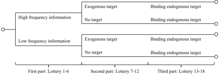
replicating Myopic Loss Aversion within the experiment. Participants were therefore split into one high-frequency and one low-frequency feedback group. They then received a fixed endowment per lottery over which they made a discrete investment decision with a positive expected return. Moving beyond existing literature, in a second and third part of the experiment two additional treatments were introduced. In part two, half of the participants were informed about the average expected return as an exogenous target and in part three all of them were given the choice to commit themselves to an endogenous, self-selected target. Compared to field experiments which had to infer reference points from behavior (Camerer et al., 1997) and previous laboratory experiments that explicitly ask for personal targets (Abeler et al., 2011; Gill and Prowse, 2012), in my design, I introduced exogenous reference points to the participants. By not relying on self-selected reference points his modification helped to overcome endogeneity issues of the previous targeting literature. Figure 1: Experiment structure
High frequency information
Low frequency information
Exogenous target
Exogenous target No target
No target
Binding endogenous target Binding endogenous target
Binding endogenous target Binding endogenous target
7
3.1. Participants
Four experimental sessions were conducted from April 2nd to April 5th, 2018 at Nova SBE with
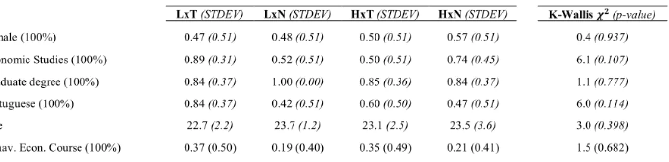
a total of 79 students participating, 50.6% of which were female. Students were invited through a posting on “Facebook”. For each master’s program, an individual group existed on this social media platform, hence targeting every master’s student at Nova SBE equally by publishing the invitation. Participants were aged between 18 and 35, with a mean of 23.5 years. 88.6% of the participants already graduated from their bachelor while only 11.4% were undergraduates and took notice of the experiment through personal referrals. Due to the nature of the undertaking, two-thirds of the participants were economics students, while only one-third studied management or finance. Additionally, 27.8% of the participants attended a behavioral economics class during their studies. Further, 58% of the participants were Portuguese, while the rest consisted of diverse nationalities, including mainly German, Italian, Brazilian and Norwegian students. Table 6 in the appendix displays the population composition per treatment. Based on a Kruskal-Wallis distribution test, randomization of participants was only close to failing for study majors and nationalities.
3.2. Experimental design
After the start of the experiment, participants had to decide on their individual investment in a sequence of eighteen identical and independent lotteries structured in three parts of six lotteries. In every round, participants received an endowment of 10 experimental credit units (ECUs), on which they had to decide in discrete steps (only full ECUs) which amount they wanted to invest in each lottery. The part of the endowment not invested was added to their payoff after the experiment. As it was not allowed to accumulate endowments over several lotteries, the maximum investment per lottery was 10 ECUs. Every lottery had a 2/3 probability of losing this amount and a 1/3 probability of winning 2.5 times the investment, creating a positive expected return. Participants were informed before the experiment about these winning and losing probabilities and the corresponding payoffs.
8
The first twelve lotteries of the experiment focused on two different manipulations that have been tested in four different treatments: Treatment H (“high-frequency information”) vs. treatment L (“low-frequency information”) was introduced before the first lottery, whereas treatment T (“suggestion of an exogenous target”) vs. treatment N (“no suggestion of an exogenous target”) was added before lottery seven. In the first manipulation under treatment H, the participants played the lotteries one by one. Before lottery one, they had to choose how much of their endowment of 10 ECUs to bet in the lottery and were informed about the realization of the lottery afterward. Next, they could decide on how much of their second endowment of again 10 ECUs to bet for lottery two, and so on. Hence, in this treatment participants made six betting decisions over the course of the first part of the experiment. In treatment L, participants played the lotteries in blocks of three with investments restricted to be equal in order to mimic a single decision. At the beginning of lottery one, subjects decided how much of their 10 ECUs endowment to bet in lottery one, two, and three. After participants committed to their investments, they were informed about the realizations for this bundle of lotteries and were thus not able to assign a gain or loss to a particular lottery, but rather to the combined result. This was repeated for lotteries four, five and six. The idea behind the design of the two treatments was to manipulate the evaluation period: In treatment L, both the frequency of choice and the information feedback were lower than in treatment H and thus participants were expected to evaluate the outcome of their allocation more aggregated. If they were myopic loss averse, they should have refused to invest more in the high-frequency lotteries.
In the second part of the experiment, half of the participants from both information frequency treatments were informed before lottery seven, that the expected return over an evaluation period of six lotteries was 70 ECUs when betting the entire endowment. Participants were told that they could consider following this exogenous target but whether or not they reached it had no further consequences. The other half of the participants served as a control group and didn’t receive this
9
information, leading to the four different treatment groups HxT (“high-frequency information and exogenous target”), HxN (“high-frequency information and no target”), LxT (“low-frequency information and target”) and LxN (“low-frequency information and no target”). Assuming rational investment strategies, neither information frequency nor the provision of an exogenous target should affect individual behavior and participants would bet their full endowment every lottery. However, both the theory on reference points, where individuals evaluate gains and losses not based on their absolute value but rather related to a usually self-selected benchmark as well as the empirical results following Camerer et al. (1997) let us expect that participants would be affected by targets and decide differently. Advantageous over their applied endogenous reference points, an exogenous target might affect individual behavior efficiently and free of endogeneity issues. Further, the effect of an extension of the evaluation period could potentially be stronger than the impact Myopic Loss Aversion, making participants invest more (less) of their endowment in the remaining lotteries, should they realize a short-falling (overshooting) of this target.
Finally, before the third part of the experiment, all participants were also encouraged to commit themselves to an endogenous, self-selected target for lotteries thirteen to eighteen. They were informed that if they selected a target, hitting or overshooting it will reward them with a bonus of 5% on exactly the target amount, while failing to do so will not result in a reward but leave the rest of their return untouched. The bonus size itself was chosen to be relevant to make participants actually think about what they could potentially reach yet sufficiently small in order to not distort their behavior and incentivize them to invest more in every lottery just to reach the bonus payment. Additionally, with an endogenous target in the third part, the impact of a previous exogenous target on the former can be tested. Assuming rational investment strategies, no change in behavior should be observed and participants with perfect foresight should set their endogenous target equivalent to an exogenous target of 70 ECUs while adopting a corresponding investment strategy (i.e. invest
10
the full endowment of 10 ECUs every lottery). Assuming differences across participants (based on their experience, demographics and information frequency), the size of the endogenous target might vary and could have a different impact compared to the exogenous target in part two.
3.3. Remuneration and participant incentives
Unlike the initial experiment by Gneezy and Potters (1997), the earned ECUs were not directly converted into real money after the experiment. Instead, they worked as lottery tickets to win a monetary reward with chances strictly increasing in the ECUs earned relatively to the other participants. 25€ were therefore available for each of the four treatments groups, as in accordance with the experiment’s theory the payoffs between the treatment groups were expected to be different. Participants were made aware of the following scheme before the experiment:
E(X) = Σ𝐸𝐶𝑈*+,*-*,./0
Σ𝐸𝐶𝑈/001/23*4*1/+35 ∗ 25€
In order to further increase individual engagement, drinks were prepared as a show-up bonus and ECUs could be performance dependent converted into sweets and fruits after the experiment: A chocolate bar, an apple or a banana were available for 60, a cookie or a peach for 20 and five gummy bears or nuts for 5 ECUs. Therefore, the total ECUs were rounded to the next full five.
3.4. Experimental procedure
Four experiment sessions (one per sub-treatment HxT, HxN, LxT, LxN) were administrated in a classroom by pen and paper with participants seated sufficiently far apart. An assistant supported the conduct of the experiment by distributing the instructions and related questionnaires to the participants upon their arrival. After the procedure was explained by the experimenter, participants could examine the instructions privately, record their ID on the questionnaire and ask questions. Participants were then instructed to record their first bets. Win letters randomly placed on top of
11
the questionnaire determined their win or loss in every lottery with an almost equal number of participants assigned to win letter A, B or C. To determine the lottery outcome, three balls marked with A, B or C were drawn from a bag. After participants recorded their lottery investment, the ball which determined the winning letter for every lottery was drawn. If a participant’s win letter did (did not) match the letter on the ball, he or she won (lost) the lottery. As only one of the three balls matched a participant’s win letter the probability of winning (losing) a lottery was 1/3 (2/3). For the high-frequency treatment, the selected ball was put back before the draw for the next lottery happened. The same procedure was repeated three times in a row for the low-frequency treatment.
After every lottery under high-frequency and every third lottery under low-frequency treatment participants calculated and recorded their earnings on the questionnaire. These calculations were checked by the experimenter in order to avoid cheating and to ensure that everyone understood the procedure. Before each of the three experiment parts, participants were informed about changes in the modalities. After lottery eighteen, participants were asked to sum up the three parts and their bonus (in case they reached their endogenous target). When setting their own target for the third part, participants had to note it down on their questionnaire before lottery thirteen. For those affected, the exogenous target was printed on the questionnaire stating the optionality to follow.
3.5. Predicted behavior: Theoretical model
Assuming that they are affected by Myopic Loss Aversion, participants weight a loss of x higher than an equal gain of x, illustrated by a weight of λ > 1 in accordance with Kahneman and Tversky (1979) and Gneezy and Potters (1997). An individual investment utility function can thus be:
With 𝐸<𝑈*(𝑥)> as an aggregated distribution value of all independent lottery draws in treatment i, the expected utility for a participant under the high-frequency treatment for an investment x is thus:
12
which is for a positive x and any 𝜆G ≤ 1.25 greater than 0. When comparing to the low-frequency
information treatment where the outcome is evaluated only every third period, the expected utility:
of the invested part of the endowment is again greater than 0 for a positive x and any λI ≤ 1.56.
When half of the participants are asked in the second part of the experiment to follow the expected return as an exogenous target, the evaluation period for both the affected high and low-frequency information treatments extends to six lotteries and hence the expected investment utility becomes:
𝐸<𝑈J(𝑥)> = 1 729∗ (15𝑥) + 12 729∗ (11.5𝑥) + 60 729∗ (8𝑥) + 160 729∗ (4.5𝑥) + 240 729∗ (𝑥) − 𝜆JS192 729∗ (2.5𝑥) + 64 729∗ (6𝑥)T
which is again greater than 0 for a positive x and any 𝜆J ≤ 1.84, allowing even more loss aversion. According to this theoretical model, a longer evaluation period tolerates a higher loss aversion that still allows a positive investment in every lottery. A necessary assumption behind this theory is, that Langer and Weber (2008) and not Bellemare et al. (2005) holds and that Myopic Loss Aversion is driven by the evaluation period and rather than commitment. Assuming sufficient computational skills, participants that evaluate their decisions over a prolonged period could thus diminish their loss averse behavior and profit from an increase in expected return (since the latter is positive).
When participants set their own target in part three, they evaluate again the λ-adjusted expected return over six lotteries but now also receive a potential bonus q on their endogenous target T:
𝐸<𝑈U(𝑥)> = V
𝐸<𝑈J(𝑥)> + 𝑞𝑇 𝑖𝑓 𝐸(𝑥) ≥ 𝑇 𝐸<𝑈J(𝑥)> 𝑖𝑓 𝐸(𝑥) < 𝑇
This is done by a small fixed percentage addition of q%, that should be of a real size yet still considerably small, in order to make the participants reveal their true target and actually follow it
𝐸<𝑈G(𝑥)> =1 3∗ (2.5x) − 𝜆G 2 3∗ (x) 𝐸<𝑈I(𝑥)> = 1 27∗ (7.5) + 6 27∗ (4) + 12 27∗ (0.5) − 𝜆I 8 27∗ (3)
13
but not externally incentivize them to target higher they feel reasonable just by an additional effect of the reward itself. Applying a presumably non-distorting 5% bonus on the exact commitment, the expected utility with a target around an expected mean return is again a positive value for all 𝜆U ≤ 1.88, allowing only for a marginally higher loss aversion than under the exogenous target.
After considering loss aversion under different evaluation periods, the question arises how much of their endowment participants are expected to invest in each lottery. Under risk neutrality, the entire endowment would be invested due to the lottery’s positive expected return. Not observing this in the previous experiments, it is most plausible to compare only the investment difference between treatments. Based on the previously determined loss aversion weights 𝜆*, projections are:
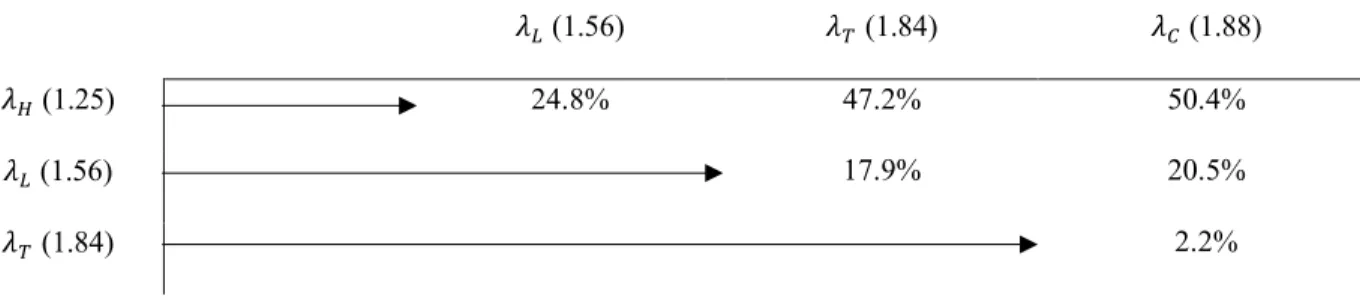
Figure 2 can be interpreted along the following figurative example: Assume that there is a population of 100 individuals with loss aversion coefficients of different magnitude and uniformly distributed from 1.00 to 2.00. Then 25% (𝜆G = 1.25) of the overall endowment of this population will be invested under the high-frequency treatment, 56% (𝜆I = 1.56)will be invested under a low
frequency-treatment, and 84% (𝜆J = 1.84) or 88% (𝜆U = 1.88) will be invest with an exogenous or endogenous target. Yet the invested endowment increases sizeable when changing from a high-frequency to a low-high-frequency treatment (24.8%)or from either one an exogenous target (47.2% and 17.9% respectively), the change within the two target types is at 2.2% rather neglectable and in practice probably non-distortive. If the real 𝜆* is smaller than 𝜆I, we should not see an effect of
targeting on the low-frequency participants as only the high-frequency participants will catch up. Figure 2: Projected change in invested endowment for different degrees of Loss Aversion
𝜆I (1.56) 𝜆J (1.84) 𝜆U (1.88)
𝜆G (1.25) 24.8% 47.2% 50.4%
𝜆I (1.56) 17.9% 20.5%
14
4. Experimental results: The impact of targeting on Myopic Loss Aversion
In the following descriptive analysis, the endowment invested per experiment part and in blocks of three lotteries, is compared across the four different sub-treatments. Table 1 presents the average invested endowment per treatment as well as the related Mann–Whitney distribution test results.
In order to draw comparisons between and within the three experiment parts that go beyond descriptive results, repeated OLS estimations are performed: Part-based with variables aggregated over six lotteries (Table 2) and block-based with an aggregation over three lotteries (Table 7 in the appendix). While the former is the focus of the analysis, the latter serves as a minimum aggregation level as participants under low-frequency feedback are forced to invest three lotteries ahead. OLS is preferred over fixed effects with regressors varying within the experiment and further necessary due to an otherwise low validity of a panel data model with only 79 participants. Yet a Hausman test rejects heteroskedasticity (1% level), estimations use clustered standard errors on a participant level to account for the fact that individual investments are not independent between lotteries.
Table 1: Average ECUs of the endowment invested per lottery on the treatment level
Invested Endowment Mann-Whitney z
(ECUs with STDEV italic below) (two-tailed significance levels with p-values italic below)
LxT LxN HxT HxN LxT|LxN HxT|HxN LxT|HxT LxN|HxN LxN|HxT LxT|HxN . Part 1 5.974 5.976 4.517 4.184 0.273 0.253 1.704 2.173 1.740 2.270 2.870 2.981 3.187 2.875 0.785 0.800 0.088 0.030 0.082 0.023 . Lotteries 1-3 5.789 5.905 4.117 3.947 0.222 0.155 -1.816 2.137 1.811 -2.148 2.955 3.177 3.405 2.976 0.825 0.877 0.069 0.033 0.070 0.032 . Lotteries 4-6 6.158 6.048 4.917 4.421 -0.027 -0.634 -1.172 1.742 1.245 -1.808 3.060 3.025 3.156 3.071 0.978 0.526 0.241 0.082 0.213 0.071 . . Part 2 6.289 6.333 6.458 4.474 0.123 1.917 -0.142 2.052 -0.211 1.698 3.114 2.763 3.275 2.661 0.902 0.055 0.887 0.040 0.833 0.090 . Lotteries 7-9 5.947 6.048 6.317 4.281 0.206 -2.005 0.483 1.686 -0.238 -1.422 3.358 3.201 3.132 2.542 0.837 0.045 0.629 0.092 0.812 0.155 . Lotteries 10-12 6.632 6.619 6.600 4.667 -0.028 -1.727 0.115 2.100 -0.186 -1.879 2.967 2.519 3.752 3.008 0.978 0.084 0.908 0.036 0.853 0.060 . . Part 3 6.289 6.071 6.15 4.316 -0.343 1.790 0.086 1.725 0.013 1.890 3.501 2.874 3.356 2.695 0.732 0.074 0.932 0.085 0.990 0.059 . Lotteries 13-15 6.053 6.190 6.250 4.228 0.028 -1.949 0.115 2.002 -0.093 -1.441 3.763 3.172 3.310 2.706 0.978 0.051 0.909 0.045 0.926 0.150 . Lotteries 16-18 6.526 5.952 6.050 4.404 -0.622 -1.580 -0.418 1.413 -0.158 -1.883 3.747 3.138 3.662 3.018 0.534 0.114 0.676 0.158 0.874 0.060 . . N 19 21 20 19 40 39 39 40 41 38
15
4.1. First part: Testing of Myopic Loss Aversion
In the first part, I replicate Gneezy and Potters (1997) by comparing average investments under high-frequency (HxT, HxN) and low-frequency information (LxT, LxN). The investment within the same feedback frequency is not significantly different (Table 1), rejecting the distribution test null hypothesis, both, by part and in blocks of three lotteries. When comparing investments between feedback frequencies, the null hypothesis can be rejected at the 10% level in all four part-based tests as well as in six of eight block-part-based tests, which might attributable to the small sample.
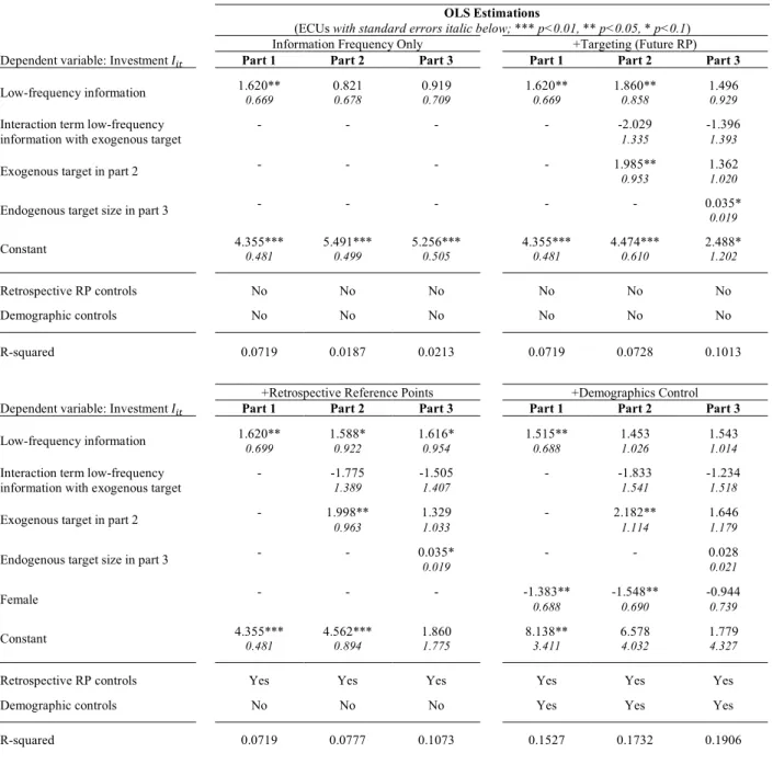
Table 2: Impact of feedback frequency and targeting on the investment per part
.
OLS Estimations
(ECUs with standard errors italic below; *** p<0.01, ** p<0.05, * p<0.1)
Dependent variable: Investment 𝐼*3
Information Frequency Only
+Targeting (Future RP)
Part 1 Part 2 Part 3 Part 1 Part 2 Part 3
.
Low-frequency information 1.620** 0.821 0.919 1.620** 1.860** 1.496
0.669 0.678 0.709 0.669 0.858 0.929
.
Interaction term low-frequency information with exogenous target
- - - - -2.029 -1.396
1.335 1.393
.
Exogenous target in part 2 - - - - 1.985** 1.362
0.953 1.020
.
Endogenous target size in part 3 - - - 0.035* 0.019
. Constant 4.355*** 0.481 5.491*** 0.499 5.256*** 0.505 4.355*** 0.481 4.474*** 0.610 2.488* 1.202 Retrospective RP controls No No No No No No Demographic controls No No No No No No . . . R-squared 0.0719 0.0187 0.0213 0.0719 0.0728 0.1013
Dependent variable: Investment 𝐼*3
+Retrospective Reference Points +Demographics Control
Part 1 Part 2 Part 3 Part 1 Part 2 Part 3
Low-frequency information 1.620** 0.699 1.588* 0.922 1.616* 0.954 1.515** 0.688 1.453 1.026 1.543 1.014
.
Interaction term low-frequency information with exogenous target
- -1.775 -1.505 - -1.833 -1.234
1.389 1.407 1.541 1.518
.
Exogenous target in part 2 - 1.998** 0.963 1.329 1.033 - 2.182** 1.114 1.646 1.179
.
Endogenous target size in part 3 - - 0.035* 0.019 - - 0.028 0.021
.
Female - - - -1.383** 0.688 -1.548** 0.690 -0.944 0.739
.
Constant 4.355*** 0.481 4.562*** 0.894 1.860 1.775 8.138** 3.411 6.578 4.032 1.779 4.327
Retrospective RP controls Yes Yes Yes Yes Yes Yes
Demographic controls No No No Yes Yes Yes
.
.
16
For empirical testing, the invested endowment 𝐼*3 of individual i in part t, is regressed on low
frequency treatment dummy 𝐿, a time constant vector of demographic controls 𝜁* (age, gender, nationality, studies, behavioral economic experience) and in the block-based case also on 𝑅*3,a set of retrospective reference points (successful previous lotteries and overall accumulated earnings):
𝐼*3 = 𝛽`+ 𝛽a𝐿 + 𝛽b𝑅*3+ 𝛽c𝜁*+ 𝑢*3 (I) When including low-frequency information as the only explanatory variable, the result of the point estimator is significant at the 5% level for the first part only (Table 2), while the constant is significant at the 1% level for all three parts, thus matching the descriptive results. Though size and direction of both the constant and the low-frequency treatment are matching the descriptive results, the explanatory power of the model is rather low for all three experiment parts. Testing block-based (Table 7), the effect of low-frequency information is larger and more significant for lotteries one to three than four to six with the explanatory power of the model remaining unchanged. Based on the clear results of the first part, Myopic Loss Aversion is assumed to be evident in this experiment.
4.2. Second part: The impact of an exogenous target on Myopic Loss Aversion
After introducing the exogenous target in the second part, the invested endowment increases strongly for the affected high-frequency information participants compared to the previous part and the other groups. This is best described as a “complete catching up” of participants affected by high-frequency information feedback with their low-frequency information peers. These results also support Langer and Weber (2008) who argue that Myopic Loss Aversion is driven by the evaluation period rather than by commitment. Yet this should be carefully evaluated since they use a slightly different experimental design. As there is no increased investment observed for the low-frequency feedback group, the true loss aversion 𝜆* of the theoretical model might actually be
smaller than 𝜆I (1.56). An implication of this insight could be that individual foresight actually
goes beyond a preassigned lottery evaluation period. Differences in the investment size between and within treatments are mostly significant at the 10% level for both part and block-based testing.
17
Empirically, regression I is extended by the effect of the exogenous target 𝛽e. Block-based, the
impact of a potential short-falling 𝛽f is additionally included, with 𝑆*3 indicating the earnings from lottery seven to nine (in case of significance, loss aversion around a target might be underlying):
𝐼*3 = 𝛽`+ 𝛽a𝐿 + 𝛽b𝑅*3+ 𝛽c𝜁* + 𝛽e𝑇 + 𝛽h𝑇𝐿 + 𝛽f(𝑇 − 𝑆*3) + 𝑢*3 (II) For the second part of the experiment, a significant effect (5% level) of the exogenous target is observed, making affected participants invest on average almost two ECUs more than their peers. After adding the exogenous target, size and significance (5% level) of the low-frequency feedback treatment, as well as the explanatory power of the model for part two, also increase. Testing block-based, the exogenous target effect is prevalent only for lotteries seven to nine, while the impact of feedback frequency remains unchanged. Yet both impact and size of the low-frequency treatment increased for part two, this should not be overinterpreted, as the size of its interaction term with the target is indicative that this effect is reversed for the “LxT” treatment group. Without a significant distance-to-target effect, loss aversion around an exogenous target cannot be supported (Table 7).
4.3. Third part: The impact of an endogenous target on Myopic Loss Aversion
In the third part, when participants are encouraged to follow a self-selected, endogenous target, the average investment does not change significantly compared to the previous parts. Comparing the size of the endogenous target set between high frequency (58.3) and low frequency (62.2) participants, no significant difference is observed between them, though it is at the 5% level when comparing between those who had an exogenous target before (55.3) and those who have not had (65.3). 76 of 79 participants did not feel any discouragement and selected an exogenous target, of which 46 reached their goal and received the corresponding bonus. Yet differences between the treatments do not change significantly to the second part, when testing part-based, more significant differences are lost when testing block-based. With most significance losses happening in the last lottery block, the two types of targets might work differently, not least as an endogenous target is apparently not enough for those treated with “HxT” to catch up with their peers in the third part.
18
In the last step, regression II is extended by the endogenous target size, while keeping the exogenous target T as a control. In the block-based case, similar to regression II, from lotteries sixteen to eighteen, the model is again extended by the impact of a potential target short falling 𝛽i:
𝐼*3 = 𝛽` + 𝛽a𝐿 + 𝛽b𝑅*3+ 𝛽c𝜁* + 𝛽e𝑇 + 𝛽h𝑇𝐿 + 𝛽f𝐶*+ 𝛽i(𝐶* − 𝑆*3) + 𝜀*3 (III)
Part-based testing shows that on a 10% significance level, the investment per lottery in the third part increases by 0.035 ECUs for each ECU higher endogenous target size chosen. Similar to the exogenous target, this effect is stronger and more significant (5% level) for lotteries thirteen to fifteen but insignificant for lotteries sixteen to eighteen when testing block-based. One possible explanation for both significance losses could be that individuals lose sight on their target when being influenced by realized outcomes and thus should be remembered repeatedly about them. An additional beneficial trait of the endogenous target is also a gender-specific effect, as an otherwise persistent higher female loss aversion disappears in part three. Despite not entirely replicating the descriptive results without applying additional controls, results are confirmative that an exogenous target helps to overcome Myopic Loss Aversion while an endogenous target alone is not sufficient.
With a significant impact of the endogenous target size on the investment, it should also be of interest what determines the commitment. Equation IV regresses the endogenous target size 𝐶* on the feedback frequency 𝐿, the exogenous target T, previous earnings 𝛱* and demographics 𝜁*:
𝐶* = 𝛽` + 𝛽a𝐿+𝛽b𝜁* + 𝛽c𝑇 + 𝛽e𝛱* + 𝜀* (IV) Yet, the exogenous target does not have a direct impact on the investment in the third part under part-based testing, there is however an impact at the 1% significance level on the endogenous target size but no significant impact of the feedback frequency (Table 3). Those provided in part two with an exogenous target on average aim over nine ECUs higher in the third part, and thus come closer to the exogenous target size of 70 ECUs. Significant at the 1% level, women target almost eleven ECUs less than their male peers, which will be further discussed in the robustness check section.
19
Besides a lucky streak, the probability of reaching the endogenous target 𝐸𝑅* might also depend
on further individual traits, including most of the previous dependent and independent variables. This question is analyzed by a probit model and benchmarked with a linear probability model:
𝐸𝑅* = 𝛽` + 𝛽a𝐿+𝛽b𝜁* + 𝛽c𝑇 + 𝛽e𝛱* + 𝛽h𝐶*+ 𝛽f𝐼̅* + 𝜀* (V) Interpreting the marginal effect at means of the probit model (Table 4), chances for those treated by high-frequency feedback reaching the endogenous target increase by 24% when provided with an exogenous target before but decrease by 10% (24%-34%) for those affected by low-frequency feedback previously, which could be related to the different evaluation horizons of the two groups. Also, participants with higher earnings in the previous parts of the experiment are less likely to reach their target. This could be explained by overconfident behavior caused by previous success.
Table 3: Selected endogenous target size
OLS Estimations Dependent variable:
Endogenous target size 𝐶*3
(*** p<0.01, ** p<0.05, * p<0.1)
Point Estimator (absolute ECUs) Robust Standard Error
..
Low-frequency information 2.915 4.070
.
Exogenous target in part 2 9.323** 3.612
. Female -10.550*** 3.636 . Constant 81.792** 37.236 . . .
Retrospective RP controls Yes
Demographic controls Yes
R-squared 0.2507
Table 4: Probability of bonus reached
OLS Estimations Probit Estimations (MEAM)
Dependent variable:
Probability of bonus reached 𝐸𝑅*
(*** p<0.01, ** p<0.05, * p<0.1) (*** p<0.01, ** p<0.05, * p<0.1)
Point Estimator Robust SE Point Estimator Robust SE
Average investment in part 3 -0.012 0.020 -0.009 0.016
.
Low-frequency information 0.047 0.156 0.007 0.159
.
Low-freq. information/exog. target -0.374 0.229 -0.339* 0.198
..
Exogenous target in part 2 0.217 0.181 0.241* 0.140
.
Endogenous target size in part 3 0.002 0.003 0.002 0.003
.
Total previous earnings -0.006*** 0.001 -0.009*** 0.002
.
Constant 1.504** 0.670 - -
.
Retrospective RP controls Yes Yes
Demographic controls Yes Yes
20
4.4. Robustness checks
The following section discusses the robustness of feedback frequency and reference points for different controls. While the early literature (Gneezy and Potters, 1997; Bellemare et al., 2005) mainly argued based on descriptive results, later authors (Haigh and List, 2005; Fellner and Sutter, 2009; Hopfensitz and Wranik, 2008) control for robustness by OLS and fixed effect estimations.
4.4.1. Retrospective reference points
As a first robustness check, retrospective reference points have been included. Participants might not only be affected by their expectations but also by their previous experiences. Hopfensitz (2009) finds in the context of Myopic Loss Aversion evidence for a Gamblers Fallacy, a behavioral bias when individual investment is increased after favorable results of previous lotteries. In my experiment though, I cannot detect an impact of previously accumulated earnings on any testing level. Surprisingly I observe a Reversed Gamblers Fallacy (Table 7), with significantly lower investments in the first part after successful previous lotteries: It might be that economics students assess the probability of consecutive successful lotteries differently or that individual targeting behavior actually exists, and individuals prefer riskless savings when the target is within reach. Yet they are mostly insignificant, controlling for retrospective reference points improves the model’s explanatory power while decreasing size and significance of the feedback frequency for lotteries four to twelve, underlining the varsity of effects that determine individual investment decisions.
4.4.2. Demographic characteristics
With most of the literature applying fixed effect models, little is known about the impact of demographic traits on the investment. Following Table 6 in the appendix, individual characteristics are randomly distributed across treatments. When accounting for them, one of the most interesting insights of my research is that women not only target lower before the third part, as already mentioned but also invest around 1.5 ECUs less over the first two parts while only catching up with
21
their male peers in part three. Empirically, a higher female loss aversion is among others confirmed by Schmidt and Traub (2002). Decreasing female loss aversion is probably the biggest advantage of the exogenous target over the exogenous one. Further, the model is robust for other demographic traits and increased in explanatory power. Not least, when testing block-based after applying all controls, with a significant distance-to-endogenous target effect, results are speculative for a loss aversion around an individual endogenous target, supporting the proposal of Camerer et al. (1997).
4.4.3. Endogeneity issues in the third part
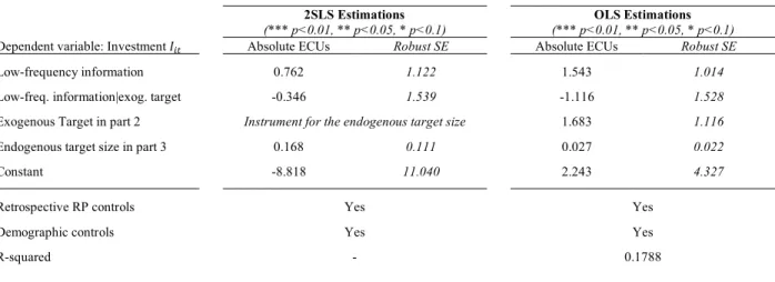
As participants that invest more logically also aim for a higher return, endogeneity caused by reverse causality between the endogenous target and the investment size might be observed. A solution at hand for this is an instrumental variable approach using the exogenous target from the second part to exactly identify the former. Since there is no significant impact of the exogenous target on the investment size in the third part, exogeneity of the instrument is evident. Knowing from previous results (Table 4) that the exogenous target significantly impacts the endogenous target size, the necessary instrumental relevance is also presumed. Coefficients, however, remain insignificant (though they change in size) when performing the 2SLS estimation (Table 5). Further, a Durbin-Wu-Hausman test fails to reject exogeneity null hypothesis of the endogenous target size, hence the endogenous target size is – against the meaning of its name – not entirely endogenous. Despite different target sizes, a “common sense” between the treatments might be not too far apart.
Table 5: IV of the third part of the experiment (endog. target size instrument by exog. target)
2SLS Estimations OLS Estimations
Dependent variable: Investment 𝐼*3
(*** p<0.01, ** p<0.05, * p<0.1) (*** p<0.01, ** p<0.05, * p<0.1)
Absolute ECUs Robust SE Absolute ECUs Robust SE
..
Low-frequency information 0.762 1.122 1.543 1.014
.
Low-freq. information|exog. target -0.346 1.539 -1.116 1.528
Exogenous Target in part 2 Instrument for the endogenous target size 1.683 1.116
.
Endogenous target size in part 3 0.168 0.111 0.027 0.022
.
Constant -8.818 11.040 2.243 4.327
.
. .
Retrospective RP controls Yes Yes
Demographic controls Yes Yes
22
5. Conclusion
This thesis presented a behavioral economic laboratory experiment on the impact of prospective reference points on Myopic Loss Aversion and was conducted with 79 students at Nova SBE. Following a design based on Gneezy and Potters (1997), I added insights on targeting behavior discovered by Camerer et al. (1997) to the original experiment. In line with the literature, evidence for Myopic Loss Aversion was found through a treatment with different information frequencies.
Assigning the exogenous target only to a part of the participants, the goal was to assess whether an artificially prolonged evaluation period helps individuals to invest more of their endowment in the lottery. Consequently, I showed that those affected by high-frequency feedback and provided with an exogenous target in the second part managed to completely catch up with the low-frequency feedback group. Against predictions of the theoretical model, the latter did not increase their investment, giving room to speculate that there might be some kind of individual foresight. My results can also carefully be interpreted to support Langer and Weber's (2008) findings, who show that in fact the evaluation period drives Myopic Loss Aversion and not the commitment horizon.
Those who previously have had an exogenous target also selected a higher endogenous target and are more likely to reach it, supporting the hypothesis that prospective reference points reduce
Myopic Loss Aversion. Yet an endogenous target is not enough to overcome myopic behavior, it
helps to surpass an otherwise persistent female loss aversion, though they still target less than men. After including demographics and retrospective reference points, I find evidence supporting loss aversion around the endogenous target, which is – against the implications of its name – exogenous.
Though the effect of targeting is pointing towards the hypothesized direction, it is important to note that like in all laboratory experiments, issues of external validity might remain with both the endowment type and the participant group not being representative, leaving room to repeat the setup with more participants, a real monetary endowment or in a context outside of the university.
23
If the proposed effects are valid and Myopic Loss Aversion is truly reduced by prospective reference points, agents invested in assets with varying evaluation periods should be encouraged to assess their investment strategy rather based on its contribution to a long-term goal than on recent developments. This insight could help not only managers to guide their investment professionals in the evaluation of financial returns but also policymakers to provide such targets to their citizens when designing private pension and healthcare saving plans. The results of this experiment suggest that the equity premium puzzle can be partially solved by applying more individual foresight.
6. Literature
Abeler, Johannes, Armin Falk, Lorenz Goette, and David Huffman. 2011. “Reference Points and Effort Provision.” American Economic Review 101 (2): 470–92.
https://doi.org/10.1257/aer.101.2.470.
Bellemare, Charles, Michaela Krause, Sabine Kröger, and Chendi Zhang. 2005. “Myopic Loss Aversion: Information Feedback vs. Investment Flexibility.” Economics Letters 87 (3): 319–24. https://doi.org/10.1016/j.econlet.2004.12.011. Benartzi, Shlomo, and Richard Thaler. 1995.
“Myopic Loss Aversion and the Equity Premium Puzzle.” Quarterly Journal of
Economics 110 (1): 73–92.
https://doi.org/10.2307/2118511.
Beshears, John, James J. Choi, David Laibson, and Brigitte C. Madrian. 2017. “Does Aggregated Returns Disclosure Increase Portfolio Risk Taking?” Review of Financial Studies 30 (6): 1971–2005. https://doi.org/10.1093/rfs/hhw086. Camerer, Colin, Linda Babcock, George
Loewenstein, and Richard Thaler. 1997. “Labor Supply of New York City Cabdrivers: One Day at a Time.” The Quarterly Journal of
Economics 112 (2): 407–41.
https://doi.org/10.1162/003355397555244. Crawford, Vincent P, and Juanjuan Meng. 2011.
“New York City Cabdrivers ’ Labor Supply Revisited : Reference-Dependent Preferences with Rational-Expectations Targets for Hours and Income.” American Economic Review 101 (5): 1912–32.
https://doi.org/10.1257/aer.101.5.1912. Doran, Kirk. 2014. “Are Long-Term Wage
Elasticities of Labor Supply More Negative than Short-Term Ones?” Economics Letters 122 (2). Elsevier B.V.: 208–10.
https://doi.org/10.1016/j.econlet.2013.11.023.
Eriksen, Kristoffer W., and Ola Kvaløy. 2010a. “Do Financial Advisors Exhibit Myopic Loss Aversion?” Financial Markets and Portfolio
Management 24 (2): 159–70.
https://doi.org/10.1007/s11408-009-0124-z. ———. 2010b. “Myopic Investment Management.”
Review of Finance 14 (3): 521–42.
https://doi.org/10.1093/rof/rfp019.
Farber, Henry S. 2005. “Is Tomorrow Another Day? The Labor Supply of New York City
Cabdrivers.” Journal of Political Economy 113 (1): 46–82. https://doi.org/10.1086/426040. ———. 2008. “Reference-Dependent Preferences
and Labor Supply: The Case of New York City Taxi Drivers.” American Economic Review 98 (3): 1069–82.
https://doi.org/10.1257/aer.98.3.1069. Fehr, Ernst, and Lorenz Goette. 2007. “Do Workers
Work More If Wages Are High? Evidence from a Randomized Field Do Workers Work More If Wages Are High? Evidence from a
Randomized Field Experiment.” The American
Economic Review 97 (1): 298–317.
https://doi.org/10.1257/aer.97.1.298.
Fellner, Gerlinde, and Matthias Sutter. 2009. “Causes, Consequences, and Cures of Myopic Loss Aversion–An Experimental Investigation.” The
Economic Journal 119 (537): 900–916.
https://doi.org/10.1111/j.1468-0297.2009.02251.x.
Gill, David, and Victoria Prowse. 2012. “A Structural Analysis of Disappointment Aversion in a Real Effort Competition.” American Economic
Review 102 (1): 469–503.
https://doi.org/10.1257/aer.102.1.469. Gneezy, Uri, Arie Kapteyn, and Jan Potters. 2003.
“Evaluation Periods and Asset Prices in a Market Experiment.” Journal of Finance 58
24
(2): 821–37. https://doi.org/10.1111/1540-6261.00547.
Gneezy, Uri, and Jan Potters. 1997. “An Experiment on Risk Taking and Evaluation Periods.” The
Quarterly Journal of Economics 112 (2): 631–
45. https://doi.org/10.1162/003355397555217. Haigh, Michael S, and John A List. 2005. “Do
Professional Traders Exhibit Myopic Loss Aversion? An Experimental Analysis.” The
Journal of Finance 60 (1): 523–34.
https://doi.org/10.1111/j.1540-6261.2005.00737.x.
Heijden, Eline van der, Tobias J. Klein, Wieland Müller, and Jan Potters. 2012. “Framing Effects and Impatience: Evidence from a Large Scale Experiment.” Journal of Economic Behavior
and Organization 84 (2). Elsevier B.V.: 701–
11. https://doi.org/10.1016/j.jebo.2012.09.017. Hopfensitz, Astrid. 2009. “Previous Outcomes and
Reference Dependence : A Meta Study of Repeated Investment Tasks with and without Restricted Feedback.” TSE Working Paper
Series. Vol. 87.
http://econpapers.repec.org/paper/tsewpaper/22 194.htm.
Hopfensitz, Astrid, and Tanja Wranik. 2008. “Psychological and Environmental Determinants of Myopic Loss Aversion.”
MPRA Working Paper.
http://mpra.ub.uni-muenchen.de/9305/1/MPRA_paper_9305.pdf. Kahneman, Daniel, and Amos Tversky. 1979.
“Prospect Theory: An Analysis of Decision under Risk.” Econometrica: Journal of the
Econometric Society 47 (3): 263–91.
https://doi.org/10.1111/j.1536-7150.2011.00774.x.
———. 1984. “Choices, Values, and Frames.”
American Psychologist, no. 39: 341–50.
https://doi.org/10.1037/0003-066X.39.4.341.
Köszegi, Botond, and Matthew Rabin. 2006. “A Model of Reference-Dependent Preferences.”
Quarterly Journal of Economics 152 (4): 1133–
65. https://doi.org/10.1093/qje/qjt005.Advance. Langer, Thomas, and Martin Weber. 2008. “Does
Commitment or Feedback Influence Myopic Loss Aversion?. An Experimental Analysis.”
Journal of Economic Behavior and Organization 67 (3–4): 810–19.
https://doi.org/10.1016/j.jebo.2006.05.019. Mehra, Rajnish, and Edward C. Prescott. 1985. “The
Equity Premium: A Puzzle.” Journal of
Monetary Economics 15 (2): 145–61.
https://doi.org/10.1016/0304-3932(85)90061-3. Pope, Devin G., and Maurice E. Schweitzer. 2011. “Is
Tiger Woods Loss Averse? Persistent Bias in the Face of Experience, Competition, and High Stakes.” American Economic Review 101 (1): 129–57. https://doi.org/10.1257/aer.101.1.129. Schmidt, Ulrich, and Stefan Traub. 2002. “An
Experimental Test of Loss Aversion.” The
Journal of Risk and Uncertainty 25 (3): 233–
49. https://doi.org/10.1023/A:1020923921649. Sutter, Matthias. 2007. “Are Teams Prone to Myopic
Loss Aversion? An Experimental Study on Individual versus Team Investment Behavior.”
Economics Letters 97 (2): 128–32.
https://doi.org/10.1016/j.econlet.2007.02.031. Thaler, Richard, Amos Tversky, Daniel Kahneman,
and Alan Schwartz. 1997. “The Effect of Myopia and Loss Aversion on Risk Taking: An Experimental Test.” The Quarterly Journal of
Economics 112 (2): 647–61.
https://doi.org/10.1162/003355397555226. Tversky, Amos, and Daniel Kahneman. 1992.
“Advances in Prospect-Theory - Cumulative Representation of Uncertainty.” Journal of Risk
and Uncertainty 5 (4): 297–323.
https://doi.org/Doi 10.1007/Bf00122574. 7. Appendix
7.1. Additional statistical tables
Table 6: Distribution of demographic characteristics over the four treatment groups
LxT (STDEV) LxN (STDEV) HxT (STDEV) HxN (STDEV) K-Wallis 𝝌𝟐 (p-value)
. Female (100%) 0.47 (0.51) 0.48 (0.51) 0.50 (0.51) 0.57 (0.51) 0.4 (0.937) .. Economic Studies (100%) 0.89 (0.31) 0.52 (0.51) 0.50 (0.51) 0.74 (0.45) 6.1 (0.107) . Graduate degree (100%) 0.84 (0.37) 1.00 (0.00) 0.85 (0.36) 0.84 (0.37) 1.1 (0.777) . Portuguese (100%) 0.84 (0.37) 0.42 (0.51) 0.60 (0.50) 0.47 (0.51) 6.0 (0.114) . Age 22.7 (2.2) 23.7 (1.2) 23.1 (2.5) 23.5 (3.6) 3.0 (0.398) .
Behav. Econ. Course (100%) 0.37 (0.50) 0.19 (0.40) 0.35 (0.49) 0.21 (0.41) 1.5 (0.682)
25
Dependent var.: Investment 𝐼*3
OLS Estimations
(robust standard errors in italic; *** p<0.01, ** p<0.05, * p<0.1) Information frequency only
L 1-3 L 4-6 L 7-9 L 10-12 L 13-15 L 16-18 . Low-frequency information 1.816*** (0.698) 1.424** (0.685) 0.675 (0.702) 0.967 (0.706) 0.860 (0.741) 0.977 (0.769) .. Constant 4.034*** (0.506) 4.675*** (0.494) 5.325*** (0.481) 5.658***(0.561) 5.265*** (0.506) 5.248*** (0.548) . Retrospective controls No No No No No No Demographic controls No No No No No No R-squared 0.0810 0.0532 0.0118 0.0240 0.0172 0.0206
Dependent var.: Investment 𝐼*3
+Targeting (Forward-looking RP)
L 1-3 L 4-6 L 7-9 L 10-12 L 13-15 L 16-18
Low-frequency information 1.816*** (0.698) 1.424** (0.685) 1.766* (0.910) 1.952** (0.888) 1.617 (0.980) 1.356 (0.955)
..
Low-freq. information/ex. target - - -2.136 (1.383) -2.011 (1.420) -1.866 (1.444) -0.964 (1.502)
Exogenous target in part 2 - - 2.036** (0.911) 1.189 (1.654) 1.393 (1.005) 1.319 (1.104)
Distance to exogenous target - - - 0.020 (0.032) - -
Endogenous target size in part 3 - - - - 0.047** (0.021) 0.005 (0.023)
Distance to endogenous target - - - 0.032 (0.021)
Constant 4.034*** (0.506) 4.675*** (0.494) 4.280*** (0.582) 4.667*** (0.694) 1.791 (1.257) 3.415** (1.310)
Retrospective controls No No No No No No
Demographic controls No No No No No No
R-squared 0.0810 0.0532 0.0651 0.0820 0.1250 0.0977
Dependent var.: Investment 𝐼*3
+Retrospective Reference Points
L 1-3 L 4-6 L 7-9 L 10-12 L 13-15 L 16-18
..
Low-frequency information 1.782** (0.698) 0.715 (1.004) 2.074 (1.277) 2.058 (1.448) 1.571 (1.102) 0.507 (1.128)
..
Low-freq. information/ex. target - - -2.491 (1.748) -2.171 (1.401) -1.610 (1.700) -0.132 (1.566)
Exogenous target in part 2 - - 2.110** (0.983) -0.145 (1.861) 1.905* (1.051) 1.116 (1.074)
Distance to exogenous target - - - 0.062 (0.041) - -
Endogenous target size in part 3 - - - - 0.058** (0.026) -0.031 (0.030)
Distance to endogenous target - - - - - 0.093** (0.040)
Success in previous lottery -0.897 (0.700) -1.831* (1.109) 0.221 (1.461) 0.540 (1.384) 0.258 (1.007) 0.002 (0.011)
Constant 4.471*** (0.628) 5.727*** (1.085) 3.520 (2.379) 3.331 (2.377) 0.349 (1.884) 1.810 (2.384)
. .
Retrospective controls Yes Yes Yes Yes Yes Yes
Demographic controls No No No No No No
R-squared 0.1006 0.0976 0.0705 0.1043 0.1536 0.1454
Dependent var.: Investment 𝐼*3
+Demographic Controls
L 1-3 L 4-6 L 7-9 L 10-12 L 13-15 L 16-18
Low-frequency information 1.736*** (0.719) 0.368 (1.187) 1.970 (1.359) 1.883 (1.520) 1.775 (1.089) 0.604 (1.145)
..
Low-freq. information/ex. target - - -2.286 (1.898) -2.393 (1.515) -1.718 (1.688) 0.124 (1.502)
Exogenous target in part 2 - - 2.223* (1.152) 0.963 (2.215) 2.672*** (1.122) 1.548 (1.184)
Distance to exogenous target - - - 0.035 (0.046) - -
Endogenous target size in part 3 - - - - 0.050* (0.021) -0.015 (0.026)
Distance to endogenous target - - - 0.070* (0.038)
Success in previous lottery -1.235* (0.744) -2.307* (1.234) 0.903 (1.522) 0.312 (1.507) 0.257 (1.070) -1.277 (1.112)
Female -1.419** (0.722) -1.390* (0.727) 1.673*** (0.770) -1.563** (0.759) -0.675 (0.807) -0.935 (0.820)
Constant 9.762** (4.178) 9.548** (4.801) 5.990 (0.529) 4.041 (4.550) 3.900 (4.740) 0.179 (4.803)
. .
Retrospective controls Yes Yes Yes Yes Yes Yes
Demographic controls Yes Yes Yes Yes Yes Yes
26
7.2. Additional figures
Figure 3: Development of the experimental history on Myopic Loss Aversion
Authors Country (town) & method Observations High /Low #Rounds endowment/lottery € value of the Main MLA findings Gneezy and
Potters (1997) Netherlands (Tilburg); paper and pencil 41/42 students 12 0.90€
Baseline experiment, proof of the underlying of Myopic
Loss Aversion (MLA) Gneezy et al.
(2003)
Netherlands (Tilburg, Amsterdam);
Computer
40/40 traders 15 0.90€ Under MLA market prices of risky financial assets are significantly higher
Bellmare et al.
(2005) Netherlands (Tilburg); computer 44/44 students 9 0.70€
MLA is persistent even if the
information frequency is disentangled from decision making
Haigh and List (2005)
US (University of Maryland); paper and
pencil 32/32 students 27/27 financial markets trader 9 0.80€ (students) 3.20€ (traders)
Professional traders exhibit
MLA to a greater extent
than students
Sutter (2007) Germany (Jena); computer 64/62 students 28/28 teams 9 1.00€
Team decision making reduces MLA but cannot completely overcome it
Langer and
Weber (2008) Germany (Mannheim); computer 54/53 students 30
25€ for the entire experiment (self- allocation/lottery)
If the feedback is separated from commitment, only the latter affects MLA strongly
Hopfensitz and Wranik (2008)
Switzerland (Geneva);
Computer 38/39 students 15 0.90€
MLA stronger when initial
investment round lead to loses
Fellner and
Sutter (2009) Germany (Jena); computer 30/30 students 18 0.5€
Both investment horizon and feedback frequency contribute equally to MLA
Eriksen and
Kvaøy (2010a) Norway (Stavanger); computer
80/80 students 24/26 financial
advisors
9 0.25€ (students) 1.00€ (fin. advisors)
Financial advisors exhibit
MLA to a greater extent
than students
Eriksen and
Kvaøy (2010b) Norway (Stavanger); computer 205/205 students 9 0.25€ MLA also exists over other participants endowment
Van der Heijden et al. (2012) Netherlands (countrywide); computer 551/551 citizens (representative for population)
3 2.00€ More impatient people are
stronger affected by MLA
Beshears et al. (2017)
US (Harvard
University); computer 160/160 students 18 1.60€ MLA is not persistent if the experiment is conducted with real financial assets
Own Work Project (2018)
Portugal (Lisbon);
paper and pencil 39/40 students
18 0.20€
(approximate material value)
Exogenous targets can help to overcome MLA and set a higher endogenous target
27
7.3. Experiment instructions
Dear Student,
Thank you again for coming today and welcome to this experimental session! For a smooth procedure of the experiment, I would kindly ask you to carefully read the instructions below and follow them as strictly as possible.
Just be yourself: Take the time to think and answer to the best of your capabilities. There is no wrong answer and there are no tricks. All your answers will be treated with the uttermost care and all your responses will be completely anonymous!
During the experiment, it is not allowed to communicate with other participants. If you have a question, please raise your hand and we will approach you in silence. If a question is relevant for other participants, we will answer it aloud for everyone.
You should have 4 pages, something to write and a calculator. Please fill in your 5-digit student ID and your name on top of the sheet.
Part one (read out loud before lottery seven)
This experiment is structured as a betting game with 18 successive lotteries and is divided into three parts with six lotteries each. In each lottery, you will start with an amount of 10 Experimental Credit Units (ECUs). You must decide which part of this amount (between 0 and 10 ECUs) you wish to bet in each of in the following lotteries. You have a chance of 2/3 (67%) to lose the amount you bet and a chance of 1/3 (33%) to win two and a half times the amount you bet. You are requested to record your choice on your questionnaire. Suppose that you decide to bet an amount of X ECUs (0 ≤ X ≤ 10) in the lottery. Then you must fill in the amount X in the column headed “Bet amount” for every lottery. The remaining amount (10-X) you note in “Saved amount”.
Only for the low-frequency treatment: Also, you fix your choice for the next three lotteries. Thus,
if you decide to bet an amount X in the lottery 1, then you also bet an amount X for the following lotteries 2 and 3. Therefore, three consecutive lotteries are joined together on the questionnaire. Whether you win or lose in the lottery depends on your personal win letter. This letter is indicated on top of your questionnaire. Your win letter can be A, B or C, and is the same for all 18 lotteries. In any round, you win the lottery if your win letter matches the lottery letter randomly drawn by the assistant (each with a probability of 1/3), and you lose vice versa if your win letter does not match. Please always record the letter drawn by the assistant in the column “Outcome of lottery”. ___________