Measuring air quality with low-cost sensors in citizen science applications

(1)

-

Measuring Air Quality with Low-Cost Sensors

in Citizen Science Applications

(2)

Measuring Air Quality with Low-Cost Sensors in Citizen Science

Applications

Dissertation supervised by Thomas Bartoschek (Ifgi) Roberto Henriques (Nova IMS)

Sven Casteleyn (UJI).

(3)

ACKNOWLEDGMENTS

I would like to express my very great appreciation to my supervisor Thomas Bartoschek for his enthusiastic encouragement and useful critiques of this research work. His motivation is contagious and has been very much appreciated.

I am also very grateful to my co-supervisors Dr. Roberto Henriques and Dr. Sven Casteleyn for sharing with me meaningful feedback for the improvement of this thesis.

I would like to sincerely thank Dr. Marco Painho for his guidance and support, and my honest thanks to the Erasmus Mundus Program of the European Commission for providing me the scholarship to accomplish this Master’s program.

My grateful thanks are also extended to all the administrative staff at the University of Münster and Universidade Nova de Lisboa for helping to make this Master’s program run smoothly.

This Master was an intense academic and personal experience in my life. I would like to give thanks to all the special friends I made during this time. Each one of them is a valuable part on it.

I also wish to thank my parents and my brother for always being there for me. To my Brazilian friends and family, thank you for your support and encouragement throughout my studies.

(4)

DECLARATION

I hereby declare that I am the sole author of this Master Thesis entitled “Measuring Air Quality with Low-Cost Sensors in Citizen Science Applications”.

I declare that this thesis is submitted in support of candidature for the Master of Science in Geospatial Technologies and that it has not been submitted for any other academic or non-academic institution.

______________________________ Jana Lodi Martins

(5)

ABSTRACT

Air pollution is unquestionably a public health emergency, and the rates of pollution continue to rise at an alarming rate in cities all over the world. Nevertheless, the traditional monitoring equipment is very expensive, and the available measurements are not sufficient to precisely classify air quality in several locations in a city. Recent advancements in air quality measuring technology provide a potential opportunity to increase the air quality data, and to raise public awareness of health issues arising from air pollution. This study focuses on the development and evaluation of a new prototype for the monitoring of fine particulate matter (PM2.5). It describes the design approach and the evaluation methods, in which a series of field experiments were conducted to evaluate the performance of the prototype and of a commercial low-cost device in comparison with a reference monitor. The results showed that the prototype presented a good performance in environments with a high variation of particle concentrations (variations above 100µg/m³), such as cooking-environments and exposure to cigarette smoke, for most of the experiments (R² = 0.55-0.85). However, their agreement was very poor in environments without high variability of particle concentrations. The performance comparison between identical sensors purchased in the same year revealed a very high agreement (R² = 0.92), but prototypes which utilized sensors acquired in different years presented a very weak correlation in most of the experiments. The analysis of the commercial low-cost device’s performance revealed a moderate to strong linear correlation with the reference monitor in all the experiments (R= 0.51-0.93); this study also demonstrates that the maximum limit of detection of the device was much lower than the value given by the manufacturer (approximately 180µg/m³, in contrast to the value of 400µg/m³). For applications of real-time measurements, the prototype developed in this research may be especially utilized as indicative of PM2.5 hotspots and trends in ambient conditions, primarily in residences, monitoring the frequency and duration of high exposure events, such as cooking, smoking, and biomass burning. Nevertheless, this research demonstrates the necessity for individual sensor performance testing prior to field use, and that presumptions about the representativeness of measurements of PM2.5 carried out by low-cost sensors should be made with caution.

(6)

ACRONYMS API - Application Program Interface

AQE - Air Quality Egg AQI - Air Quality Index CO - Carbon monoxide

CSV - Comma Separated Value DIY - Do-It-Yourself

EPA - United States Environmental Protection Agency EU – European Union

FEM - Federal Equivalent Method GPS - Global Positioning System ifgi - Institute for Geoinformatics

LANUV - Landesamt für Natur, Umwelt und Verbraucherschutz LED - Light-emitting diode

Pb - Lead

NO - Nitrogen oxide NO2 - Nitrogen dioxide

NOX - Mono-nitrogen oxides (NO and NO2) O3 - Ozone

PM - Particulate matter

PM10 - Coarse particulate matter PM2.5 - Fine particulate matter Ppb - Parts per billion

Ppm - Parts per million

R - Linear correlation coefficient R² - Coefficient of determination RTC - Real-Time-Clock

SO2 - Sulfur Dioxide

VGI - Volunteered Geographic Information WAQI - World Air Quality Index

(7)

INDEX

1 INTRODUCTION 11

1.1 Aim and Specific Objectives 12

1.1.1 Aim 12

1.1.2 Specific Objectives 12

1.2 Context of this Research 13

1.3 Thesis Structure 13

2 THEORETICAL BACKGROUND 14

2.1 Air Quality 14

2.1.1 Air Pollutants 14

2.1.2 Air Quality Legislation in Europe 16

2.1.3 Air Quality Index 17

2.2 Citizen Science in Air Quality 19

2.2.1 Sensors for Air Quality 19

2.2.2 Existing Air Quality Platforms 22

2.2.3 Comparison of Online Platforms 24

3 METHODOLOGY 26

3.1 Development of the Prototype 26

3.1.1 Prototype Components 26

3.1.2 Prototype Operation 30

3.1.3 Case Design 30

3.2 Experiments 31

3.2.1 Description of the Experiments 31

(8)

3.3.2 Assessment Methods 34 4 RESULTS 36 4.1. Experiment 1 36 4.2 Experiment 2 37 4.3 Experiment 3 38 4.4 Experiment 4 39 4.5 Experiment 5 40 4.6 Experiment 6 40 4.7 Data Completeness 41 5 DISCUSSION 42 5.1 Main Findings 42

5.1.1 Performance of the Prototypes 42

5.1.2 Comparison of Identical Sensors 43

5.1.3 AirBeam Performance 44

5.1.4 Analysis of the Data considering the EU Directive and the EPA 46

5.1.5 Data Completeness Analysis 46

5.2 Limitations 47

5.2.1 Monitor Reference 47

5.2.2 Data Limitations 48

6 CONCLUSION AND FUTURE WORK 49

(9)

INDEX OF TABLES

Table 1: Summary of some common air pollutants (Adapted from EPA, 2014) ... 14

Table 2: Potential effects of common air pollutants (Adapted from EPA, 2014) ... 15

Table 3: Important limit values according to Directive 2008/50/EC ... 16

Table 4: Data quality objectives for ambient air quality assessment (Adapted from EU, 2008) ... 17

Table 5: Description of potential uses for low-cost air sensors (EPA, 2014) ... 20

Table 6: Suggested Performance Goals for Sensors for several applications by EPA (EPA, 2014) ... 21

Table 7: Comparison between existing air quality platforms ... 24

Table 8: Components of the prototype ... 27

Table 9: Specifications of the Shinyei PPD42NS ... 29

Table 10: Summary of the experiments ... 31

Table 11: Technical specifications: TSI DustTrak 8534 Handheld (TSI, 2014) ... 33

Table 12: Technical specifications: AirBeam ... 33

Table 13: Linear correlation (R) and coefficients of determination (R²) for Experiment 1 ... 37

Table 19: Data Completeness Analysis ... 41

Table 20: Summary of the agreement of the prototypes with DustTrak ... 42

(10)

INDEX OF FIGURES

Figure 1: Location of the monitoring stations and PM2.5 concentration according to the WHO database

(World Health Organization, 2016) ... 11

Figure 2: AQI levels of health concern (USEPA, 2014) ... 18

Figure 3: Real Time Air Quality Index website ... 18

Figure 4: Air Quality Egg device and web platform... 22

Figure 5: Smart Citizen device and web platform ... 23

Figure 6: Air Casting device and web platform ... 23

Figure 7: Methodological Approach ... 26

Figure 8: Prototype ... 27

Figure 9: Arduino board ... 28

Figure 10: SenseBox-Shield ... 28

Figure 11: Schematic showing how the particle sensor operates (USEPA, 2015) ... 29

Figure 12: Inside the Shinyei PPD42NS ... 29

Figure 13: Prototype operation flow ... 30

Figure 14: Example of a log file of the prototype ... 30

Figure 15: Example of one experiment ... 32

Figure 16: Time series graphs for Experiment 1 ... 36

Figure 18: Time-series graphs for Experiment 3 ... 38

Figure 22: AirBeam time series without averaging in Experiment 3... 45

(11)

1 INTRODUCTION

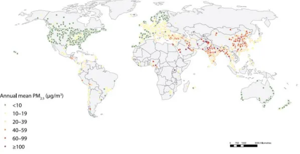
According to the World Health Organization (WHO), air pollution is the world´s largest environmental health risk, and it is estimated that around 1.4 billion urban residents in the world live in areas with air pollution above recommended air quality guidelines (World-Health-Organization, 2016). Air pollution affects all regions, socio-economic and age groups. The organization assesses the global exposure to air pollution based on the concentration of fine particulate matter (PM2.5), and Figure 1 presents the location of the monitoring stations and PM2.5 concentration according to the database of the organization.

Figure 1: Location of the monitoring stations and PM2.5 concentration according to the WHO database (World Health Organization, 2016)

Although some government agencies monitor and publish metropolitan air quality data and indexes, there are several limitations to this approach. In general, the spatial resolution of the pollution sampling is very poor and frequently the use of mathematical models is necessary to estimate pollutant concentrations over vast sections of the cities, which can be both inaccurate and complex (Sivaraman et al, 2013). Furthermore, the traditional monitoring equipment necessary to meet the standards established by national regulations for air quality has high costs of acquisition and maintenance (Devarakonda et al., 2013; Velasco et al, 2016).

In this context, the low-cost air quality measuring systems for participatory sensing emerge as a potential solution for the worldwide air quality measuring issue. These systems are small devices that include sensors capable of collecting and transmitting environmental measurements in real time, with low costs and involving participation

(12)

pollution information to citizens and raise public awareness of health issues arising from air pollution.

However, while public interest is quickly growing, the data quality of the air sensors remains uncertain, particularly that of commercial devices which may be utilized by citizens and communities to measure air quality in their local environments (Jiao et al., 2016). Further research on low-cost air quality sensors is essential, in order to get additional insight into the specific influence of environmental and operational conditions on the performance of low-cost sensors (Holstius, 2014).

In order to advance the research on the topic, this study will focus on the development of a new prototype for the monitoring of fine particulate matter (PM2.5). This document describes the design approach and process up to the point of building and testing the instrument. It presents the results of an evaluation of the developed prototype and of a commercial low-cost device (AirBeam) in a series of field experiments, which validated the performances of the instruments with a reference monitor (DustTrak).

1.1 AIM AND SPECIFIC OBJECTIVES

1.1.1 Aim

The aim of this work is to develop a low-cost prototype for the monitoring of fine particulate matter (PM2.5) and compare its performance with a reference monitor and with an existing low-cost device. Field experiments in the city of Münster, Germany, were undertaken in order to characterize its performance.

Research Question: Under which circumstances is it possible to obtain a good

performance of low-cost devices designed to measure fine particulate matter (PM2.5) in Citizen Science Applications?

1.1.2 Specific Objectives

 Perform a comprehensive literature review on air quality monitoring, citizen science applications in air quality and on the European legislation for air quality itself.

 Investigate the existing low-cost citizen science air quality measuring systems in the world and its user interface online platforms for the visualization of air quality data.

(13)

 Evaluate the performance of the prototype in different environments and under different conditions, through comparison with a reference instrument (DustTrak).

 Compare the performance of identical PM2.5 sensors purchased in similar and in different years, to understand the reproducibility of the sensor performance.  Analyze the performance of a commercial low-cost PM2.5 instrument

(AirBeam).

1.2 CONTEXT OF THIS RESEARCH

This study is a part of the SenseBox Project, of the Institute for Geoinformatics, University of Münster. The SenseBox is a low-cost citizen science system that enables the users to make location-based environmental measurements collected by sensors (SenseBox, 2017). Currently, the system collects data such as temperature, humidity, air pressure and noise and publishes it on an online open platform. A previous study was performed in the Institute to include pollutant measurement sensors in the device, but it found several limitations, e.g., some sensors were not able to measure very low values of pollutant concentrations, and the same type of sensors presented different results for equal locations and equal time (Pesch, 2015).

1.3 THESIS STRUCTURE

This Thesis consists of six chapters in total. In Chapter 1, objectives and research question are presented. After that, the theoretical background is stated in Chapter 2, indicating essential fundamentals of air quality and citizen science. Chapter 3 introduces the methodology for the development of the prototype and the realization of the experiments. Field tests are a central task to evaluate the performance of the developed prototype. Chapter 4 focuses on the results of the experiments conducted in different environments. The main findings and limitations of this study are presented in Chapter 5. Finally, Chapter 6 presents the conclusions of this Master’s Thesis and discusses the outcomes for possible future work.

(14)

2 THEORETICAL BACKGROUND

2.1 AIR QUALITY

2.1.1 Air Pollutants

According to the United States Environmental Protection Agency (EPA), air pollution involves a complex combination of different chemical components in different forms in the atmosphere: solid particles, liquid droplets, and gases. Some of these pollutants are temporarily in the air (i.e. hours to days), while others are long-lasting (i.e. years). The factors which influence the amount of time that a pollutant remains in the atmosphere are its reactivity with other substances and its propensity to deposit on a surface; these influences are affected by the pollutant composition and weather conditions including precipitation, temperature, wind and sunlight (Williams et al., 2014).

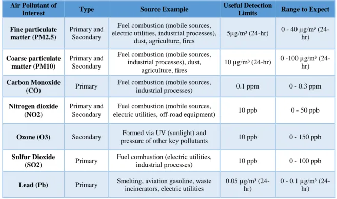
Pollutants in the atmosphere are emitted by an extensive variety of sources including natural occurrences and those of man-made origin. Examples for natural sources are dust storms, forest fires, and volcanic eruptions, while man-made sources include vehicles, gas facilities, and industries. The primary pollutants are released directly from a source (examples: carbon monoxide [CO], nitrogen dioxide [NO2], particulate matter [PM] and sulfur dioxide [SO2]); while the secondary pollutants derive from others through chemical reactions (examples: ozone [O3] and some forms of particulate matter). Table 1 presents a summary of some common air pollutants, as well as relevant information for detecting these pollutants in the air.

Table 1: Summary of some common air pollutants (Adapted from EPA, 2014) Air Pollutant of

Interest Type Source Example

Useful Detection

Limits Range to Expect Fine particulate

matter (PM2.5)

Primary and Secondary

Fuel combustion (mobile sources, electric utilities, industrial processes),

dust, agriculture, fires

5µg/m³ (24-hr) 0 - 40 µg/m³ (24-hr) Coarse particulate matter (PM10) Primary and Secondary

Fuel combustion (mobile sources, industrial processes), dust,

agriculture, fires

10 µg/m³ (24-hr) 0 -100 µg/m³

(24-hr) Carbon Monoxide

(CO) Primary

Fuel combustion (mobile sources,

industrial processes) 0.1 ppm 0 - 0.3 ppm

Nitrogen dioxide (NO2)

Primary and Secondary

Fuel combustion (mobile sources,

electric utilities, off-road equipment) 10 ppb 0 - 50 ppb

Ozone (O3) Secondary Formed via UV (sunlight) and

pressure of other key pollutants 10 ppb 0 - 150 ppb

Sulfur Dioxide

(SO2) Primary

Fuel combustion (electric utilities,

industrial processes) 10 ppb 0 - 100 ppb

Lead (Pb) Primary Smelting, aviation gasoline, waste incinerators, electric utilities

0.05 µg/m³ (24-hr)

0 - 0.1 µg/m³ (24-hr)

(15)

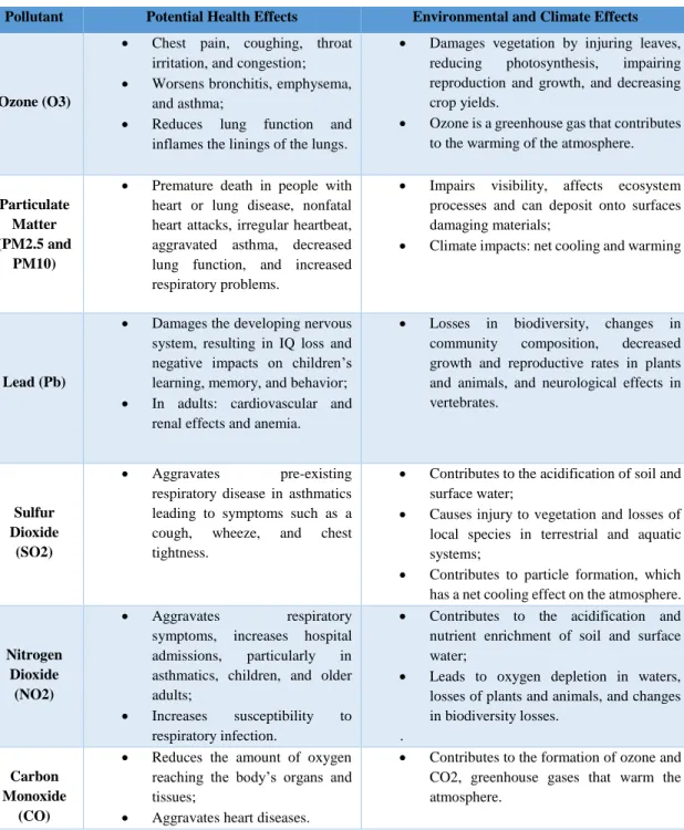
Air pollution has been associated with several issues, such as health conditions, environmental and climate effects. According to the EPA, there are six main pollutants of concern due to their huge impact, identified by the organization as the “criteria pollutant”: particulate matter (PM), carbon monoxide (CO), ozone (O3), nitrogen dioxide (NO2), sulfur dioxide (SO2), and lead (Pb) (EPA, 2016). Table 2 summarizes potential effects associated with the criteria pollutants.

Table 2: Potential effects of common air pollutants (Adapted from EPA, 2014) Pollutant Potential Health Effects Environmental and Climate Effects

Ozone (O3)

 Chest pain, coughing, throat

irritation, and congestion;

 Worsens bronchitis, emphysema,

and asthma;

 Reduces lung function and

inflames the linings of the lungs.

 Damages vegetation by injuring leaves,

reducing photosynthesis, impairing

reproduction and growth, and decreasing crop yields.

 Ozone is a greenhouse gas that contributes

to the warming of the atmosphere.

Particulate Matter (PM2.5 and

PM10)

 Premature death in people with

heart or lung disease, nonfatal heart attacks, irregular heartbeat, aggravated asthma, decreased lung function, and increased respiratory problems.

 Impairs visibility, affects ecosystem

processes and can deposit onto surfaces damaging materials;

 Climate impacts: net cooling and warming

Lead (Pb)

 Damages the developing nervous

system, resulting in IQ loss and negative impacts on children’s learning, memory, and behavior;

 In adults: cardiovascular and

renal effects and anemia.

 Losses in biodiversity, changes in

community composition, decreased

growth and reproductive rates in plants and animals, and neurological effects in vertebrates.

Sulfur Dioxide

(SO2)

 Aggravates pre-existing

respiratory disease in asthmatics leading to symptoms such as a

cough, wheeze, and chest

tightness.

 Contributes to the acidification of soil and

surface water;

 Causes injury to vegetation and losses of

local species in terrestrial and aquatic systems;

 Contributes to particle formation, which

has a net cooling effect on the atmosphere.

Nitrogen Dioxide

(NO2)

 Aggravates respiratory

symptoms, increases hospital

admissions, particularly in

asthmatics, children, and older adults;

 Increases susceptibility to

respiratory infection.

 Contributes to the acidification and

nutrient enrichment of soil and surface water;

 Leads to oxygen depletion in waters,

losses of plants and animals, and changes in biodiversity losses.

. Carbon

Monoxide (CO)

 Reduces the amount of oxygen

reaching the body’s organs and tissues;

 Aggravates heart diseases.

 Contributes to the formation of ozone and

CO2, greenhouse gases that warm the atmosphere.

(16)

2.1.2 Air Quality Legislation in Europe

The most recent legislation relating to air quality in Europe is the EU Directive 2008/50/EC of the 21th May of 2008. The Directive consolidated several earlier directives and set objectives for some pollutants which are harmful to public health and the environment, requiring the Member States to:

• Monitor and assess air quality to ensure that it meets these objectives;

• Report to the Commission and the public the results of this monitoring and assessment;

• Prepare and implement air quality plans containing measures to achieve the objectives (EU, 2008).

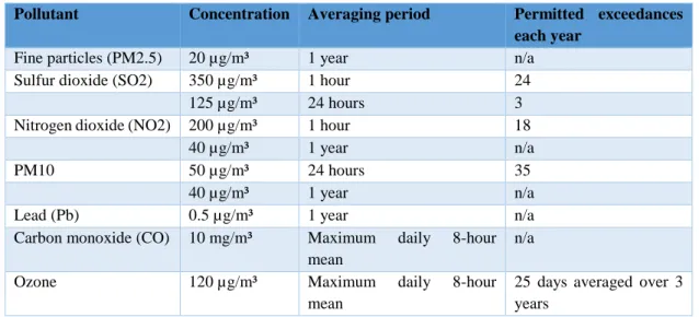
The Directive aims to protect human health and the environment, its main significance being to combat pollutants’ emissions at their origin and to identify measures to decrease emissions. As part of the policy, limits for the pollutants were determined. Table 3 presents the most important limits for compliance with the Directive. The limit values for the individual parameters are divided into annual averages and/or a specific number of hours.

Table 3: Important limit values according to Directive 2008/50/EC

Pollutant Concentration Averaging period Permitted exceedances

each year

Fine particles (PM2.5) 20 µg/m³ 1 year n/a Sulfur dioxide (SO2) 350 µg/m³ 1 hour 24 125 µg/m³ 24 hours 3 Nitrogen dioxide (NO2) 200 µg/m³ 1 hour 18 40 µg/m³ 1 year n/a PM10 50 µg/m³ 24 hours 35 40 µg/m³ 1 year n/a Lead (Pb) 0.5 µg/m³ 1 year n/a Carbon monoxide (CO) 10 mg/m³ Maximum daily 8-hour

mean

n/a

Ozone 120 µg/m³ Maximum daily 8-hour mean

25 days averaged over 3 years

Member States shall collect, interchange and propagate air quality information in order to understand better the impacts of air pollution and develop appropriate strategies. Information on concentrations of all regulated pollutants in ambient air must also be readily accessible to the public.

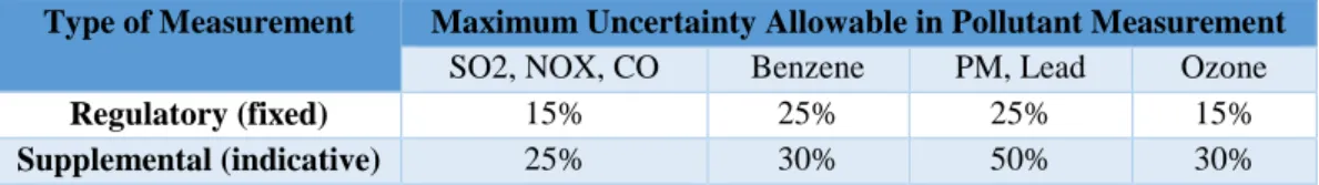
The Directive also outlines the use of “indicative measurements” that in specific conditions can be used to supplement “fixed” or “regulatory” measurements, in order to provide information on the spatial variability of pollutant concentrations. However, no provision is made for them to be used independently for regulatory purposes. These

(17)

supplementary measurements have less stringent requirements for data quality, as can be seen in Table 4.

Table 4: Data quality objectives for ambient air quality assessment (Adapted from EU, 2008) Type of Measurement Maximum Uncertainty Allowable in Pollutant Measurement

SO2, NOX, CO Benzene PM, Lead Ozone

Regulatory (fixed) 15% 25% 25% 15%

Supplemental (indicative) 25% 30% 50% 30%

Additionally, the use of supplementary techniques may also allow the reduction of the mandatory amount of fixed sampling points.

2.1.3 Air Quality Index

Air quality indexes are mostly used for citizen awareness purposes, i.e., to inform citizens about the level of air pollution severity in a simplified approach (Villani et al., 2016).

The Air Quality Index (AQI) was developed by the EPA and is currently the most widespread air index in the world. Such index reports how clean or unhealthy the air is, and which related health effects may be a concern. The AQI emphasizes the health effects people may experience within a few hours or days after breathing unhealthy air. The index considers the following pollutants: ground-level ozone, particulate matter, carbon monoxide, and sulfur dioxide (USEPA, 2014).

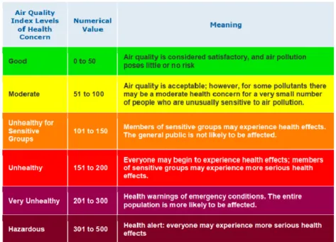
The AQI is divided into six levels of health concern varying in a scale of 0-500, according to Figure 2. The higher the AQI value, the greater the concentration of air pollution. In addition to a pure value, the AQI also offers a behavioral recommendation and a risk assessment for different groups of people. For instance, AQI values lower than 50 represent good air quality with little harm or no potential harm to public health, while AQI values over 300 represent a hazardous level of air quality and the entire population may experience serious health effects.

(18)

Figure 2: AQI levels of health concern (USEPA, 2014)

The website http://waqi.info/ presents an interactive map with the AQI derived from available information in stations worldwide (WAQI, 2017). The data relies on monitoring stations run by the governments, thus, no data from Do-It-Yourself (DIY) stations or similar are displayed and evaluated. The website is pictured in Figure 3.

(19)

2.2 CITIZEN SCIENCE IN AIR QUALITY

Citizen Science is the worldwide engagement of millions of individuals, many of them nonscientists, in collecting, categorizing, transcribing, or analyzing scientific data. Projects involving citizens include a range of topics from microbiomes to native bees to air quality (Bonney et al., 2014). Although the term “citizen science” itself has only emerged in recent years, much of the existing understanding of the natural environment already results from data that has been collected, transcribed, or processed by non-scientists. In the last two decades, the number of citizen science projects has vastly expanded, as well as scientific reports and articles resulting from their data.

The field of citizen science has been rapidly growing given the advancements in the communication and information technologies. Microphones and cameras on smartphones can record data, while mobile phone tracking, GPS, and other technologies can provide location and time-synchronization (Burke et al., 2006). Moreover, the second generation of Internet, the Web 2.0, provided services for people to collaborate and share information online (Murugesan, 2007). Goodchild introduced the term “volunteered geographic information” to describe the web phenomenon of user generated content and dissemination of geographic data provided voluntarily by individuals (Goodchild, 2006).

2.2.1 Sensors for Air Quality

Recent technologies on low-cost air quality sensors have created portable and low-cost air sensor devices that have the potential to generate a dense amount of air quality data through individual use or projects in a large network of sensors (Bartonova et al., 2015; Neophytou et al., 2015). Researchers are already utilizing low-cost sensors in exploratory research, to assess the geographical variability of urban air quality (Gao et al., 2015; Levy, 2014).

2.2.1.1 Sensor Operation

There are three main types of air quality sensors, based on their principle of operation: metal-oxide, electrochemical and optical sensors. The sensing properties in metal-oxide sensors are based on the reaction between the semiconductor metal-oxide and the gases in the atmosphere, which results in changes in conductivity. This response is measured and associated with the pollutant concentration. Electrochemical sensors operate by reacting with the gas of interest and producing an electrical signal proportional to the gas concentration. The last type of sensor is the optical one, in which a light receptor detects the light scattered by particles in the airstream, and produces a low pulse as the output. The particle concentration is estimated based on the percentage of time the

(20)

Currently, low-cost sensor instruments usually utilize metal-oxide or electrochemical sensors for the measurements of gas pollutants such as CO, NO2, NO and O3. On the other hand, commercial PM sensor devices normally use laser-based or light-emitting diode (LED)-based optical detectors of particles (Jiao et al., 2016), as the one used in this study. At present, there are no commercially available devices which utilize direct mass measurement of PM, but ongoing research aims to develop a true mass measurement (Paprotny et al., 2013).

2.2.1.2 Potential Uses and Assessment of Low-cost Sensors

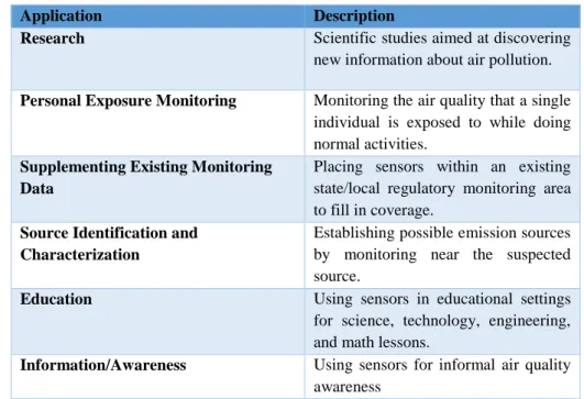
The EPA proposes several potential non-regulatory application areas for air quality sensors, which are illustrated in Table 5 (Williams et al., 2014).

Table 5: Description of potential uses for low-cost air sensors (EPA, 2014)

Application Description

Research Scientific studies aimed at discovering

new information about air pollution.

Personal Exposure Monitoring Monitoring the air quality that a single individual is exposed to while doing normal activities.

Supplementing Existing Monitoring Data

Placing sensors within an existing state/local regulatory monitoring area to fill in coverage.

Source Identification and Characterization

Establishing possible emission sources by monitoring near the suspected source.

Education Using sensors in educational settings

for science, technology, engineering, and math lessons.

Information/Awareness Using sensors for informal air quality awareness

An important aspect of the emerging low-cost technology is the method of assessment of the performance of the sensors. Although environmental agencies as EPA have a well-defined method for approving technologies for use in the regulatory process, at present there are no clear defined or universally accepted criteria to evaluate the sensors, i.e., there are no official criteria which provide a “pass” or “fail”, or alternative grading scheme to assess a particular sensor model. According to the EPA, developing such criteria will be a challenge, considering the diversity of potential applications and related performance goals (Jiao et al., 2016).

The EPA in its Air Sensor Guidebook suggests performance goals for the sensors according to the potential application, presented in Table 6. The suggestions were defined based on expert interviews, group meetings, and peer-reviewed and government related literature, and are an initial guideline to be improved over time (Williams et al., 2014).

(21)

Table 6: Suggested Performance Goals for Sensors for several applications by EPA (EPA, 2014)

Application area

Pollutants Precision Data Completeness

Rationale

I Education and Information

All > 50% ≥ 50% Measurement error is not as important as simply demonstrating that the pollutant exists in some wide

range of concentration.

II Hotspot Identification

and Characterization

All > 30% ≥ 75% Higher data quality is needed here to ensure that not only does the pollutant of interest exist in the local

atmosphere, but also at a concentration that is close to its true

value. III Supplemental Monitoring Criteria pollutants, Air Toxics

> 20% ≥ 80% Supplemental monitoring might have value in providing additional air quality data to complement existing

monitors. It must be of sufficient quality to ensure that the additional

information is helping to "fill in" monitoring gaps rather than making

the situation less understood.

IV Personal Exposure

All > 30% ≥ 80% Many factors can influence personal exposures to air pollutants. Lower precision rates make it difficult to understand how, when, and why personal exposures have occurred.

V Regulatory Monitoring

O3 > 7% ≥ 75% Precise measurements are needed to ensure high-quality data to meet

regulatory requirements. CO, SO2 > 10% NO2 > 15% PM2.5, PM10 > 10%

Furthermore, an important step to assure the data quality of the sensors is the calibration at periodic intervals, in order to assess the instrument’s response to changes in concentrations. In the calibration procedure, the instrument’s measurements are compared to a reference value under similar environmental and operational conditions as those in which the device will collect measurements, as many sensors are highly

(22)

2.2.2 Existing Air Quality Platforms

In the context of citizen science, there are several projects which collect environmental data. In most of them, environmental data is collected by low-cost sensors and then sent over the Internet to a data platform for data visualization. Examples are the AirQualityEgg, Smart Citizen, Air Casting, and the AirSensEURProject. In the following, some of these projects will be briefly presented.

2.2.2.1 Air Quality Egg

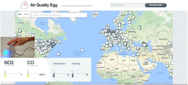
The Air Quality Egg (AQE) project aims to give citizens a way to participate in the conversation about air quality. It consists of sensing devices based on open-source hardware components and a web platform for publishing the collected data (Air Quality Egg, 2017). The device can measure concentrations of carbon monoxide and nitrogen dioxide as well as temperature and relative humidity. The enclosure indicates the air quality with different light colors. The hardware device and web platform with a selected station are shown in Figure 4.

Figure 4: Air Quality Egg device and web platform 2.2.2.2 Smart Citizen

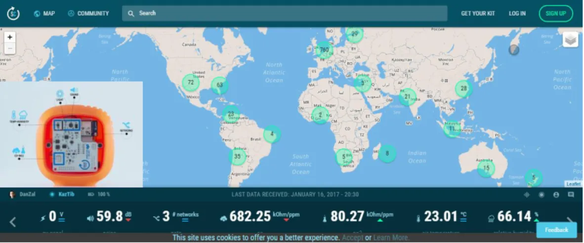
The Smart Citizen is another project which uses open source technology for citizens’ participation. Similar to the AQE approach, the platform allows participants to measure and make air quality data public. Its sensors are able to measure carbon monoxide and nitrogen dioxide concentrations, as well as temperature, brightness, humidity and noise. After configuration and deployment, the device sends data samples to a web platform, in which the data can be accessed on a map interface. Moreover, the server application offers an Application Program Interface (API), which can be used to build custom applications on top of the Smart Citizen hardware and platform (FabLab Barcelona, 2017). The hardware device and web platform are pictured in Figure 5.

(23)

Figure 5: Smart Citizen device and web platform 2.2.2.3 Air Casting

Another open-source platform for collecting, displaying, and sharing environmental data is the Air Casting. The project includes a palm-sized air quality monitor called AirBeam which is able to measure PM2.5, temperature, humidity and noise. Via Bluetooth, the measurements are sent to the AirCasting Android app, which maps and graphs the data in real time on the smartphone. Then, the data is transmitted to the AirCasting website, and the data is crowdsourced with data from other devices and heat maps are generate to indicate where PM2.5 concentrations are highest and lowest (AirCasting, 2017). As an open-source platform, the project also allows modifying its components, to include other sensors, and to transmit the data to other websites or apps. The hardware device and web platform are pictured in Figure 6.

(24)

2.2.3 Comparison of Online Platforms

Table 7 presents a comparison between several online platforms for air quality data visualization, including the following projects: Air Casting, Smart Citizen and Air Quality Egg.

Table 7: Comparison between existing air quality platforms

_{Air Casting} _{Smart Citizen} _{Air Quality Egg}

Parameters PM2.5 (µg/m³), temperature (ºC) and humidity (%)

NO2 (kOhm/ppm), CO

(kOhm/ppm), light intensity (Lux), relative humidity (%), air temperature (ºC), sound levels (dB) and battery (%)

NO2, CO, temperature and humidity

“Openness” of the projects

On the website, the data displayed is only from the AirCasting devices. It is not possible to include other devices.

The AirCasting app and website code is available on GitHub.

On the website, the data displayed is only from the Smart Citizen devices. It is not possible to include other devices. The server application offers an Application Program Interface (API), which can be used to build custom applications on top of the Smart Citizen hardware and platform

The project allows modifying its components, to include other sensors, and to transmit the data to other websites or apps.

It is not possible to include data from other devices on the

platform, only from Air

Quality Egg devices.

Operation The device collects measurements approximately once a second and sends them via Bluetooth to the smartphone, through an Android application. The app maps and graphs the data collected in real time and, at the end of each session, the data is sent to the AirCasting website.

The device collects data and sends it to a computer/ Android

App through the wireless

module installed on the data-processing board.

The device collects the data and sends it via Wi-Fi to the cloud at Opensensors.io, an open data service, which both stores and provides free access to the data. Then, the data is sent to the AQ Egg website, and to Xively, where it is possible to see graphs and other visualizations of the data.

Visualization of the data

The data from different AirCasting devices is the base for generating heat maps indicating the PM2.5 concentration.

The visualization is based on grids; each square’s color corresponds to

the average of all the

measurements recorded in that area.

It is possible to define the scale of the heat legend units on the website, changing the colors of the grids depending on the scale.

There are filters for

parameter/sensor/location/profile name/tags/time range/resolution.

There is no data interpolation, so, there is no estimation of pollutant-concentration for non-measured areas on the online map.

There are filters with which it is possible to define the kind of location (indoor/outdoor) and

the state of connectivity

(online/offline).

The units of the measurements are not clearly defined. On the website, it is informed that both units (kOhm and ppm) are utilized for the pollutants’ concentration, but there is no information about methods of conversion between these units.

The website displays the location of the devices and the last measured values, but these values are not associated with any units; so it is difficult to interpret the values and, consequentially, the air quality condition.

(25)

Download the data

The platform does not present any download option.

The platform does not present any download option. Historical

data

The platform displays historical values.

The platform does not display historical values.

(26)

3 METHODOLOGY

The following chapter describes the methodological approach adopted in this thesis, summarized in Figure 7. The following sections of this chapter will describe each of the steps stated in the figure. First, the development of the prototype will be described, which includes the prototype components, its operation, and the case design. The second section focuses on the experiments, and the third session presents the methods for treatment and assessment of the collected data.

Figure 7: Methodological Approach

3.1 DEVELOPMENT OF THE PROTOTYPE

3.1.1 Prototype Components

An illustration of the prototype is shown in Figure 8, and a list of all the components used in the prototype and its approximate costs are presented in Table 8.

Methodology 1. Development of the Prototype Prototype Components Prototype Operation Case Design 2. Experiments Description of the Experiments Instruments 3. Analytical Methods

Data Treatment Assessment _Methods

Time-Series Graph Correlation Analysis Data Compeleteness Analysis

(27)

Figure 8: Prototype

Table 8: Components of the prototype

Nr. Components: Prices

1 Arduino Uno Microprocessor 24 € 2 SenseBox – Shield (connector board) 10 € 3 Shinyei PPD42NS (PM2.5) 17 € 4 HC1000 (temperature and humidity) 14 € 5 microSD-Card 5 € 6 FAN-4010 5V 2 € 7 External Battery 10 € 8 Cables, small parts 5 €

Total 87 €

As a core, the prototype consists of a single-board microprocessor, a connector board for sensors and a sensor to measure PM2.5. These three main components will be described below.

Microprocessor: Arduino Uno

The Arduino is an open-source electronics platform based on easy-to-use hard- and software (Arduino.cc, 2017). Due to its simple and accessible user interface, the platform has been used by professionals and non-professionals in numerous interactive projects and applications. Arduino boards are capable of reading inputs and turning them into outputs, through the set of instructions that are sent to the microcontroller board. The Arduino IDE software uses the Arduino’s C-based programming language to write, edit, compile and upload the developed codes to the interface board (Evans, 2011).

(28)

and a reset button. The microcontroller board can be powered through USB or the power jack using an AC-DC adapter or battery.

Figure 9: Arduino board Connector Board: SenseBox-Shield

The SenseBox-Shield is a sensor connector board designed by the SenseBox Project. In contrast to existing connector boards available on the market, the SenseBox-Shield has different connectors for the diverse hardware interfaces provided by Arduino, and it can reduce the risk of connecting a module to the incorrect interface (Wirwahn, 2016). Moreover, it offers the possibility to store data on a MicroSD card and to provide a time stamp, which is controlled by the real-time clock (RTC), type RV8523, which has a low current consumption. A lithium battery ensures that time and date are maintained even when the device is switched off. The shield is simply plugged into the Arduino microcontroller board and can thus substitute its functionality (Pesch, 2015). An overview of the SenseBox-Shield is shown in Figure 10.

Figure 10: SenseBox-Shield PM2.5 Sensor: Shinyei PPD42NS

The Shinyei PPD42NS consists of a light chamber in which a light-emitting diode (LED) shines a light on the particles, and the amount of light that is deflected by the

(29)

particles is measured by a photodiode detector (light receptor). A resistive heater positioned at the bottom of the chamber helps to move air convectively from the bottom to the top outlet of the chamber (Austin et al., 2015).

Figure 11 illustrates the PM sensor operation, while Figure 12 presents the internal components of the sensor.

The signal processing is controlled by additional electronics, and the raw sensor output consists of low pulse occupancy (the amount of time particles are detected by the photodiode sensor), which is proportional to particle count concentration (Wang et al., 2015). The number of particles per 0.01 cubic foot can then be calculated by means of a function determined from the datasheet of the sensor (Pesch, 2015). By default, the fine particle matter concentration is not expressed in an absolute particle number per 0.01 cubic foot, but in a concentration of μg/m³. The conversion is then based on the assumption that the particles are spherical and have an average density of 1.65μg/m³ (Tittarelli et al., 2008).

The technical specifications of the sensor are presented in Table 9.

Table 9: Specifications of the Shinyei PPD42NS

Dimension W x H x D (mm) 59 x 45 x 22 Detectable PM size range ~1µm Operation voltage 5 +- 0.5 V Current consumption <90 mA Operation temperature 0 ~ 45°C Operation humidity <95% Sensitivity N/A

Output signal Pulse width modulation

Figure 12: Inside the Shinyei PPD42NS Figure 11: Schematic showing how the particle

sensor operates (USEPA, 2015)

Schematic showing how the particle sensor operates (USEPA, 2015)

(30)

3.1.2 Prototype Operation

Figure 13 presents the steps for the operation of the prototype. Once all the components are installed, it is necessary to write a code to enable the board to collect and store the data. After being uploaded to the microcontroller, the code runs in a loop successively as long as the power supply of the microcontroller is not interrupted. In order to supply the device, the prototype is charged continuously from an external battery supplying 5V power.

Figure 13: Prototype operation flow

The prototype can measure and record readings for PM2.5, temperature, and humidity, and store it on a microSD card in intervals of 15 seconds. The measured values are comma separated value files (CSV) and can be easily converted into a table of data. Each time the prototype starts to operate, it is checked if the microSD card is correctly connected. A section of a file is shown in Figure 14.

Figure 14: Example of a log file of the prototype

3.1.3 Case Design

All the components were housed in a small and portable case, made of polycarbonate, and with the following dimensions: 18x8x6cm.

In order to ensure a good aeration of the box, the laterals were perforated, as can be seen in Figure 8. In one of the sides of the case, a small fan with a volumetric flow of 12.9m³/h was installed (SUNON, 2010). Thanks to the active ventilation, the sensors inside the case were always supplied with fresh air for analysis.

All the materials, coding, as well as pictures of the prototype, can be found on:

https://github.com/janalodi/SenseBox-PM Install the components Write a code (C++) Upload code in the board Code runs in a loop Data is collected and stored

(31)

3.2 EXPERIMENTS

Several field experiments were conducted in different environments and under different conditions.

Aiming to evaluate the performance of similar PM2.5 sensors purchased in the same and in different years, 3 prototypes were built. The Prototypes 1 and 2 contain particle sensors purchased in the same year (2015), while Prototype 3 uses the same sensor, but acquired in 2016.

To evaluate the performance of the prototypes, a pair of them was co-located alongside a reference instrument (DustTrak). A commercial low-cost device (AirBeam) was also tested in all the experiments.

3.2.1 Description of the Experiments

Table 10 summarizes the experiments, their location, type, and environment, as well as their objective and duration. The experiments occurred from 06/12/2016 to 12/12/2016.

Table 10: Summary of the experiments

Experiments Local Type Environment Objective Duration Instruments

1 House Indoor Normally occupied house and cooking Measure large variations in the pollutant concentration 180 min Prototype 1 Prototype 2 DustTrak AirBeam 2 House Indoor Normally occupied house and cooking Measure large variations in the pollutant concentration 120 min Prototype 1 Prototype 3 DustTrak AirBeam 3 House Indoor Normally occupied house and smoke of cigarettes Measure large variations in the pollutant concentration 120 min Prototype 1 Prototype 3 DustTrak AirBeam

4 University Indoor Entrance of the institute Measure low concentration of pollutant 120 min Prototype 1 Prototype 3 DustTrak AirBeam

5 Center of _Münster Outdoor Christmas Market Measure high concentration of pollutant 180 min Prototype 1 Prototype 3 DustTrak AirBeam

(32)

The first three experiments had the main goal to analyze the performance of the prototype on measuring large variations of pollutant concentration. Cooking and smoking have been shown to lead to substantially elevated indoor concentrations (Wallace et al., 2011). Thus, a short series of controlled tests were performed in a residential environment.

The experiment 4 aimed to evaluate the performance in an environment with a potential low concentration of particles. It was conducted inside the building of the Institute for Geoinformatics.

The Experiments 5 and 6 were conducted in an outdoor environment, during the Christmas Market which occurred during the months of November and December in Münster. This environment is supposed to present a high concentration of particulate matter, due to a large number of people circulating in the area, as well as cigarette smoke and cooking activities.

Figure 15 presents one of the experiments conducted in this study. It is possible to see the pair of the prototypes connected to 2 external batteries, as well as the AirBeam connected to the smartphone and the DustTrak.

Figure 15: Example of one experiment

3.2.2 Instruments

More information about the reference monitor and the commercial low-cost instrument tested will be presented below.

3.2.2.1 Reference Monitor: DustTrak

The TSI DustTrak 8534 Handheld used in this study is a light-scattering laser photometer that simultaneously measures size-segregated mass fraction concentrations (PM1, PM2.5, Respirable, PM10, and Total PM fractions). It has a real-time display and can continuously log data at user-defined intervals. Data can then be exported and

(33)

analyzed in the TrakPro™ software (TSI, 2014).The instrument is capable of running for up to 6 hours; it has a concentration range of 0.001 to 150 mg/m³ and a particle size range of 0.1 to 15µm. Table 11 presents the technical specifications of the instrument.

Table 11: Technical specifications: TSI DustTrak 8534 Handheld (TSI, 2014)

Sensor Type 90° light scattering

Particle Size Range 0.1 to 15 µm

Aerosol Concentration Range 0.001 to 150 mg/m³

Operational Temp 32 to 120°F (0 to 50°C)

Storage Temp -4 to 140°F (-20 to 60°C)

Operational Humidity 0 to 95% RH, non-condensing

Time Constant User adjustable, 1 to 60 seconds

Data Logging 5 MB of on-board memory

Log Interval User adjustable, 1 second to 1 hour

Communications USB (host and device). Stored data accessible using flash memory drive

Power–AC Switching AC power adapter with

universal line cord, 115–240 VAC

3.2.2.2 Commercial PM2.5 device: AirBeam

The AirBeam is an air quality monitor which also uses a light scattering method to measure fine particulate matter. In the device, air is drawn through a sensing compartment while light from a LED bulb scatters off particles present in the airstream. The light scattered is recorded by a detector which estimates the number of particles. The collected data is sent via Bluetooth to an application on a smartphone (AirCasting, 2017). The AirBeam has a rechargeable lithium battery, which can operate for up to 10 hours. Table 12 presents the technical specifications for the AirBeam.

Table 12: Technical specifications: AirBeam

Sensor Type light scattering

Weight 7 ounces

Particle Sensor Shinyei PPD60PV

Temperature & Relative Humidity Sensor

MaxDetect RH03

Bluetooth Nova MDCS42, Version 2.1+EDR

Microcontroller Atmel ATmega32U4

Bootloader Arduino Leonardo

Time Constant ~ 1 second

(34)

3.3 ANALYTICAL METHODS

Below the methods applied to the data collected by the instruments will be described. Microsoft Excel was used for all data processing and analysis.

3.3.1 Data Treatment Methods

1) Data from all the instruments was time-matched; 2) Zero values were excluded from the database;

3) Data was aggregated in intervals of 1-minute, through the calculation of the mean, to facilitate the analysis of the results and also because the three instruments provide PM2.5 mass concentrations in different time resolutions (DustTrak and the AirBeam collected data in 1-second intervals, while the prototype in such of 15-seconds).

3.3.2 Assessment Methods

As described in section 2.2.1.2, at present there are no official criteria to evaluate air quality sensors. This study used the common practice methods found in the literature to assess the performance of the instruments utilized in this research.

1) Time-series graphs

Time-series graphs presenting the concentrations of PM2.5 over time were plotted for the instruments in all of the experiments. This type of graph is an important tool for displaying trends and changes in the data over time.

2) Correlation Analysis

To quantify and compare the strengths of the relations, correlation coefficients (R) and coefficients of determination (R²) were calculated to each pairwise dataset.

R measures the strength and the direction of a linear relationship between two variables. The value of R is such that -1≤ R ≤+1. The + and – signs are used for positive linear correlations and negative linear correlations, respectively.

R² gives the proportion of the variance (fluctuation) of one variable that is predictable from the other variable. It is a measure to determine how precise one can be in making predictions from a certain model/graph. The coefficient of determination is such that 0≤ R² ≤1.

(35)

3) Data Completeness

The total of valid data achieved from a measurement system, compared to the total that was expected to be obtained under normal and correct conditions, is called data completeness (Williams et al., 2014). This value was calculated for each instrument for all the experiments.

(36)

4 RESULTS

The following chapter presents the results of the experiments conducted in this study. For each of the 6 experiments, the time series graphs and the statistical analysis of the instruments’ performance will be presented. Then, the results for the data completeness will follow.

4.1. EXPERIMENT 1

Figure 16 presents the time series graphs for the Experiment 1. From the images, it is possible to notice that all instruments presented a substantial response to the high change of PM2.5-concentration, when the cooking was initiated approximately in minute 34. However, the concentration reported by DustTrak was consistently higher than the other instruments’ measurements. Its highest value was almost 4000μg/m³ at the peak of the experiment; while AirBeam reported 180μg/m³ and the Prototypes 1 and 2 presented 55μg/m³ and 65μg/m³, respectively. The different aspects of the AirBeam’s behavior will be further discussed in section 5.1.3.

Figure 16: Time series graphs for Experiment 1

Table 13 shows statistical summaries of linear correlation coefficients (R) and coefficients of determination (R²) for all instruments. Analysing the first coefficient, a high linear correlation was found between the reference monitor (DustTrak) and Prototype 1 (R = 0.82), as well as between the Prototype 2 and DustTrak (R = 0.78). There was a high consistency between the Prototype 1 and Prototype 2 measurements (R = 0.96 and R² = 0.92). This result can suggest a good factory calibration of the

(37)

PPD42NS sensors purchased in the same year. The data displayed by DustTrak and AirBeam exhibited less congruence (R = 0.51 and R² = 0.26).

Table 13: Linear correlation (R) and coefficients of determination (R²) for Experiment 1

DustTrak AirBeam Prototype 1

Experiment 1 R R2 R R2 R R2

AirBeam 0.51 0.26 1 1

Prototype 1 0.82 0.67 0.62 0.38 1 1

Prototype 2 0.78 0.61 0.60 0.36 0.96 0.92

4.2 EXPERIMENT 2

Figure 17 presents the time series data of DustTrak, AirBeam and Prototypes 1 and 3 in Experiment 2. From the graphs, it is possible to observe that all the devices showed an evident response to the high variation of pollutant concentration and presented two peaks, although the time series presented different behaviors. A similar trend is detectable mainly for DustTrak and Prototype 1, which will be statistically confirmed by the high linear correlation (R = 0.88). In this experiment, the correlation between AirBeam and Prototype 3 was also good (R = 0.74). The other instruments’ measurements showed less correspondence, as can be seen in Table 14.

(38)

AirBeam 0.54 0.29 1 1

Prototype 1 0.88 0.77 0.13 0.02 1 1

Prototype 3 0.42 0.18 0.74 0.55 0.19 0.04

Figure 18 illustrates the time series plots for Experiment 3, testing the effect of cigarette smoke. From the figure, the rapid increase of PM2.5-concentration can be observed, as well as a similar behaviour between DustTrak and Prototype 3 graphs. Their visual agreement is statistically verificable in Table 15, where a strong coefficient of determination was found between the instruments (R² = 0.85).

Figure 18: Time-series graphs for Experiment 3

A moderate to good agreement was revealed between the reference instrument and AirBeam and Prototype 3 (R = 0.74-0.75 and R² = 0.55-0.56), as well as between the Prototype 3 and AirBeam (R = 0.83 and R² = 0.69).

(39)

AirBeam 0.75 0.56 1 1

Prototype 1 0.74 0.55 0.25 0.06 1 1

Prototype 3 0.92 0.85 0.83 0.69 0.67 0.45

Figure 19 presents the results of the experiment conducted at the university. Visually, it is recognizable that DustTrak and AirBeam performed very similar, which can be statistically verified by the analysis of agreement. (R = 0.93 and R² = 0.86). The other instruments presented very low agreement, as illustrated in Table 16.

(40)

Figure 20 shows the performance of the instruments in the first experiment in the Christmas Market. AirBeam and DustTrak presented a moderate linear correlation and a moderate coefficient of determination (R = 0.66 and R² = 0.44). All the other instruments presented a very weak pairwise agreement (Table 17).

AirBeam 0.66 0.44 1 1

Prototype 1 0.32 0.10 0.25 0.06 1 1

Prototype 3 -0.37 0.14 -0.18 0.03 0.09 0.01

Figure 21 presents the response of the instruments in Experiment 6, also conducted at the Christmas Market. AirBeam presented a good linear correlation (0.75) and a moderate coefficient of the determination with DustTrak (0.56), while the other instruments presented a very low correlation (Table 18).

(41)

AirBeam 0.75 0.56 1 1

Prototype 1 0.24 0.06 0.21 0.04 1 1

Prototype 3 -0.16 0.03 -0.20 0.04 -0.09 0.01

4.7 DATA COMPLETENESS

Table 19 presents the results of data completeness for all the instruments in each experiment. The last column shows the weighted arithmetic mean for all the experiments, based on the duration of the tests.

Table 19: Data Completeness Analysis

Exp 1 Exp 2 Exp 3 Exp 4 Exp 5 Exp 6 All

Sensor 1 90% 53% 89% 55% 90% 48% 74%

Sensor 2 83% - - - 83%

(42)

5 DISCUSSION

This chapter focuses on the central aspects arisen in this study. The main findings and limitations are discussed in the next sections.

5.1 MAIN FINDINGS

5.1.1 Performance of the Prototypes

The main objective of this research was to analyze the performance of low-cost prototypes on measuring PM2.5 through comparison with a reference instrument. On account of this, the statistical agreements between the prototypes and the reference monitor are summarized in Table 20. It can be observed that the prototypes had a variable agreement with DustTrak in the different experiments.

Table 20: Summary of the agreement of the prototypes with DustTrak

TEST 1 TEST 2 TEST 3 TEST 4 TEST 5 TEST 6

R R2 R R2 R R2 R R2 R R2 R R2

Prototype 1 0.82 0.67 0.88 0.77 0.74 0.55 0 0 0.32 0.10 0.24 0.06

Prototype 2 0.78 0.61

Prototype 3 0.42 0.18 0.92 0.85 0 0 -0.37 0.14 -0.16 0.03

The response of the prototypes in the experiments of cooking and cigarette smoke (Experiments 1, 2 and 3) were moderate to very correlated to the reference instrument (R = 0.74-0.92 and R² = 0.55-0.85), with exception of the Prototype 3 in Experiment 2. These results suggest that the PPD42 sensor responds well in environments with high variability of particle-concentration, mainly with a creation of particles. These findings are consistent with a previous study by Wang (Wang et al., 2015), which examined the performance of 3 different low-cost sensors in a laboratory, including the one used in this study. In the referred study, particles were created by burning incense, and a very high agreement (R² = 0.95) between the instruments was registered.

A previous study in the US testing another low-cost sensor (Sharp’s Optical Dust) observed similar results in similar experiments (Olivares et al., 2012). In that study, a prototype was installed in a house and its performance was evaluated during residential activities. The results of the study also demonstrated that in these indoor environments, low-cost sensors may be useful; the prototypes responded clearly to activities like cooking and smoking of cigarettes, being capable of presenting the main trends with a good temporal resolution. In addition, another important source of indoor exposure to PM2.5 is biomass burning, where studies reported that mean daytime concentration of PM2.5 in homes using wood as fuel was nearly 3000µg/m3 (Siddiqui et al., 2009). In this sense, these sensors could be also useful in monitoring biomass cooking and/or heating events (Austin et al., 2015).

(43)

However, the performance of the prototypes developed in this study was very weak in environments with lower variations of the particle-concentration (disparities smaller than 100µg/m³, approximately), for both environments, inside the institute, and at the Christmas Market. A previous study by the Community Air Sensor Network from EPA presented consistency with these results. In the referenced study, a network of several selected sensors was tested in multiple locations for a long-term deployment, for7 months (Jiao et al., 2016). The three collocated Air Quality Egg units, which also use PPD42NS sensors, revealed poor correlation (R = 0.06-0.40) with the Federal Equivalent Method (FEM). In another study, the same particle sensors presented a nonlinear response at very high concentrations (hourly average PM2.5 ranging 77-889μg/m3) and authors used high-order models to correct their data (Gao et al., 2015). Nevertheless, other studies presented different results, e.g. the same sensors deployed in an environment with low to moderate PM2.5 concentrations (PM2.5 ranging 3-20μg/m³) revealed a good correlation with a reference monitor (R = 0.72 for 24h averages) (Holstius et al., 2014).

5.1.2 Comparison of Identical Sensors

An additional objective of this research was to compare the performance of identical sensors purchased in the same year and in different years. The results revealed that the performance agreement between the Prototypes 1 and 2, which were acquired in the same year, was very high (R² = 0.92). However, the Prototypes 1 and 3, both bought in different years, presented no correlation in any of the experiments, with exception of the smoking experiment (Test 3), which revealed a moderate linear correlation between these prototypes (R = 0.67).

In the laboratory study conducted by Wang (Wang et al., 2015), the performance of the same sensor was equivalent to the first experiment of this study, revealing a high correlation between the performance of identical sensors (R² = 0.95). Nevertheless, in the field study conducted by the EPA (Jiao et al., 2016), a comparison of identical sensors displayed a moderate agreement (R= 0.55). In a laboratory study with 20 identical sensors, Austin (Austin et al., 2015) evaluated that the response of these sensors to produced aerosol atmospheres is idiomatic, implicating that each sensor follows its own response curve.

Therefore, this study agrees with other studies to the extent that, before being used in commercialized particle monitors, each sensor requires individual calibration, since these existing systematic errors may considerably affect the measurements carried out