A decomposition approach for the p-median problem on disconnected
graphs
∗Agostinho Agra1, Jorge Orestes Cerdeira2, and Cristina Requejo3
1Departamento de Matem´atica and Centro de Investiga¸c˜ao e Desenvolvimento em Matem´atica e Aplica¸c˜oes (CIDMA),
Universidade de Aveiro, 3810-193 Aveiro, Portugal. [email protected]
2Departamento de Matem´atica and Centro de Matem´atica e Aplica¸c˜oes (CMA), Faculdade de Ciˆencias e Tecnologia,
Universidade NOVA de Lisboa, Quinta da Torre, 2829-516 Caparica - Portugal. [email protected]
3Departamento de Matem´atica and Centro de Investiga¸c˜ao e Desenvolvimento em Matem´atica e Aplica¸c˜oes, Universidade
de Aveiro, 3810-193 Aveiro, Portugal. [email protected]
Abstract
The p-median problem seeks for the location of p facilities on the vertices (customers) of a graph to minimize the sum of transportation costs for satisfying the demands of the customers from the facilities. In many real applications of the p-median problem the underlying graph is disconnected. That is the case of p-median problem defined over split administrative regions or regions geographically apart (e.g. archipelagos), and the case of problems coming from industry such as the optimal diversity management problem. In such cases the problem can be decomposed into smaller p-median problems which are solved in each component k for different feasible values of pk, and the global solution is obtained by finding the best
combination of pk medians. This approach has the advantage that it permits to solve larger
instances since only the sizes of the connected components are important and not the size of the whole graph. However, since the optimal number of facilities to select from each component is not known, it is necessary to solve p-median problems for every feasible number of facilities on each component. In this paper we give a decomposition algorithm that uses a procedure to reduce the number of subproblems to solve. Computational tests on real instances of the optimal diversity management problem and on simulated instances are reported showing that the reduction of subproblems is significant, and that optimal solutions were found within reasonable time.
Keywords: Location; optimal diversity management problem; decomposition.
1
Introduction
The p-median problem is a well-known NP-hard combinatorial optimization problem that seeks for the location of p facilities on the vertices (customers) of a network to minimize the sum of transportation costs for satisfying the demands of the customers from the facilities. See [9]
∗
for a recent survey of main results and algorithms for the p-median problem, and [14, 15] for an extensive annotated bibliography on the p-median and related problems.
In the p-median problem we are given a weighted graph G = (V, A, w), where the vertices of V = {1, . . . , n} represent locations, and (i, j) is an arc of A if and only if a facility located in i might serve location j. Each arc a = (i, j) of G has a cost wa. Let, for j ∈ V , yj be a 0-1
variable indicating whether vertex j is selected (yj = 1) or not (yj = 0) to install a facility. Let,
for (i, j) ∈ A, xij be a 0-1 variable indicating whether a facility in location represented by vertex
i will serve location j (xij = 1) or not (xij = 0).
With variables y and x the p-median problem [12] can be formulated as follows.
min X (i,j)∈A wijxij subject to (1.1) X j∈V yj = p (1.2) X (i,j)∈A xij + yj = 1, j ∈ V (1.3) xij ≤ yi, (i, j) ∈ A (1.4) yj ∈ {0, 1}, j ∈ V (1.5) xij ∈ {0, 1}, (i, j) ∈ A (1.6)
Equation (1.2) guarantees that exactly p locations are selected. Equations (1.3) state that either vertex j is selected and no arc will be incident to j, or else there will be exactly one arc incident to j. Inequalities (1.4) express that if a vertex is not selected, its outdegree is equal to zero. Finally (1.5) and (1.6) define the ranges of the variables. The problem considered here assumes that the demand at each vertex cannot be served by more than one facility.
We address the p-median problem when graph G has several different connected compo-nents. This case arises in the automotive industry, namely in the production of electric wiring configurations for vehicles, where the problem is known as the optimal diversity management problem [1, 2, 4, 5, 6]. This situation also occurs when location takes place over split adminis-trative regions or regions geographically apart (e.g. archipelagos). Thus, the p-median problem considered here can be seen as a generalization of the classical p-median problem to the case of multiple components. In what follows, independently of the context of the problem, we call facility to any element of a p-median set.
When graph G is disconnected, the p-median problem can be decomposed into q-median problems, for different feasible values of q, in each component of G, and an optimal solution can be found by optimally combining the solutions of the different components so that the number of facilities sum up to p.
This procedure has the advantage of decomposing the p-median problem on graph G into a number of subproblems of much lower sizes. The drawback is the large number of q-median subproblems that, in principle, have to be solved (in each component of G, as many as p+1 minus the number of components), which may turn the procedure impractical. However, most of these subproblems may be neglected in the search for the optimal solutions, and only a small number of
selected (active) subproblems need to be solved. In this paper we propose an exact decomposition algorithm that iterates between a procedure of elimination of subproblems, and solving a selected active subproblem. For the subproblems elimination procedure, the algorithm uses and updates, at each iteration, two matrices, one keeping the lower bounds (matrix L) and the other keeping the upper bounds (matrix U ) on the optimal values of every subproblem. Then, the bounds from these matrices are combined in a efficient procedure to reduce active subproblems. The matrix L is initialized with values from the dual of the linear relaxation. The matrix U is initialized with the values obtained from a greedy and a relax-and-fix heuristics. Computational results show that the number of problems need to be solved is very small, and the optimal solutions were obtained in reasonable times.
The paper is organized as follows. In Section 2 we review the decomposition approach for p-median problems on disconnected graphs. In Section 3 we give the procedures to derive lower bounds and upper bounds on the optimal values of the subproblems.The algorithm to reduce the number of subproblems is presented in Section 4. In Section 5 we introduce our decomposition approach for the p-median problem that uses the procedures of Sections 3 and 4. Computational tests to evaluate the performance of the algorithm on real and simulated instances are reported in Section 6, and some concluding remarks are discussed in Section 7.
2
Decomposition procedure
Suppose graph G has m > 1 connected components and assume that in each component at least one facility should be installed. We denote by K = {1, . . . , m} the set of indices of the connected components of G and by Gk = (Vk, Ak) the subgraph of G induced by component
k ∈ K.
We can adjust model (1.1)-(1.6) for disconnected graphs, introducing positive integer variables pkthat indicate the number of facilities in each component k, for all k ∈ K. We get the following
formulation. min X (i,j)∈A wijxij (2.1) subject to (1.3) − (1.6) X k∈K pk= p (2.2) X j∈Vk yj = pk, k ∈ K (2.3) pk∈ {1, 2, . . . , min{p − m + 1, |Vk|}}, k ∈ K (2.4)
More precisely, we replace equation (1.2) by equations (2.2), (2.3) and (2.4) defining pk as the
number of facilities in each component k, and ensuring that the number of facilities in the m connected components will be p.
If we knew the values of pk, say p∗k, of an optimal solution, then an optimal p-median solution
p∗k, the p-median problem can still be solved considering one connected component at a time, with the following two-phase strategy.
Phase One: solve the pk-median problem for each component k (we shall call this the (pk,
k)-subproblem) with pk varying from 1 to min{p − m + 1, |Vk|};
Phase Two: identify, among all the pk-median solutions obtained for each component k, an
optimal combination of p facilities.
The first phase reduces to solve a q-median problem, for different values of q, in each compo-nent and the problem arising in the second phase is the linking set problem (LSP) [3]. The LSP was considered for the first time, at the best of our knowledge, by Avella et al. [4] and later by Agra et al. [1], as a subproblem of the optimal diversity management problem.
The LSP is a special case of the following more general problem. Given a non-negative, r × m, matrix C = [cqk] and a positive integer p ≥ m, select exactly one element in each column of C
such that the sum of the rows’ indices equals p and the sum of the selected elements is minimum. If we consider binary variables zqk, for q ∈ {1, . . . , r} = Q and k ∈ {1, . . . , m} = K, indicating
whether element (q, k) of matrix C is selected (zqk = 1) or not (zqk = 0), the problem can be
formulated as a linear integer program as follows.
min X k∈K X q∈Q cqkzqk (2.5) subject to X k∈K X q∈Q qzqk = p (2.6) X q∈Q zqk= 1, k ∈ K (2.7) zqk∈ {0, 1}, q ∈ Q, k ∈ K (2.8)
Equation (2.6) ensures that the sum of the rows’ indices equals p. Equations (2.7) ensure that exactly one element from each column k ∈ K is selected, and (2.8) are the integrality constraints on the variables. The objective function (2.5) seeks to minimize the sum of the selected elements of matrix C.
In the LSP, r := p − m + 1; the entry cqk is the optimal value of the (q, k)-subproblem (i.e.,
q-median problem on graph Gk), for q = 1, . . . , min{r, |Vk|} and, if r > |Vk|, cqk := +∞, for
q = |Vk| + 1, . . . , r; and variables pk=Pq∈Qqzqk.
Problem (2.5)-(2.8) can be efficiently solved as a shortest path on an acyclic graph [8]. The main difficulty with this decomposition approach is the need for solving the min{p − m + 1, |Vk|} q-median problems on every component k of G, since the LSP can be solved very quickly.
In order to avoid solving all these NP-hard problems, we work with lower and upper bounds on their optimal values, and use a domination rule to discard most of these problems. In the next section we describe how these bounds are initially computed.
3
Computing initial lower and upper bounds
The decomposition algorithm that we will give for the p-median problem works on two r × m, with r = p−m+1, matrices L = [lqk] and U = [uqk], where lqkand uqkare, respectively, lower and
upper bounds on the optimal value wqk∗ of the (q, k)-subproblem, if q ≤ |Vk| and lqk= uqk= +∞,
otherwise.
The effectiveness of the decomposition algorithm strongly depends on the quality of the lower and upper bounds lqk and uqk, that should be enough close to the respective optimal values w∗qk.
However, given the large number of subproblems to address (m × (m − p + 1)), to compute L and U within acceptable time, expedite procedures should be used. Having this in mind, we delineated the strategy that we describe below.
3.1 Initial lower bounds
To compute matrix L we propose an approach that explores the structure of the dual of the linear relaxation of the p-median problem, and a certain behavior of the marginal improvements of the objective function of p-median problem, as more facilities are added.
The dual of the linear relaxation of the p-median problem (1.1)-(1.6) is (see [7]) D(p) = max {p γ + X j∈V αj} (3.1) subject to X j∈V βij− αi− γ ≤ 0 i ∈ V (3.2) βij− αj ≤ wij (i, j) ∈ A (3.3) βij ≥ 0 (i, j) ∈ A (3.4)
where γ, αj and βij are the dual variables associated with constraints (1.2), (1.3) and (1.4),
respectively.
Let (γ∗, α∗, β∗) be an optimal solution of (3.1)-(3.4). Hence, D(p) = p γ∗ +P
j∈V α∗j is a lower
bound on the optimal value of the p-median solution. As p occurs only in the objective function (3.1), it follows that (α∗, β∗, γ∗) is a feasible solution of problem D(p0) = max{p0 γ + P
j∈V αj}
subject to (3.2)-(3.4), for all values p0. Thus, for every number of facilities p0, D(p0) ≥ p0 γ∗ + P
j∈V α ∗
j, and the inequality is tight for p0= p. Letting p0 = p + t, we then have
D(p + t) ≥ D(p) + tγp∗, for t = ±1, ±2, . . . (3.5)
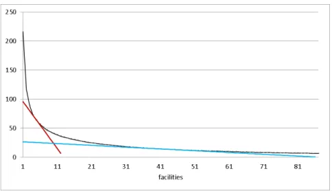
It is well known that the marginal improvement in the objective function of the p-median problem (i.e. the difference between the optimal values for q facilities and q + 1 facilities) vanishes (although it does not necessarily decrease monotonically, see [9] pg 23), when adding facilities, being much larger for small values of p than for high values of p.
The optimal dual D(p) shares the same behavior. We illustrate this behavior in Figure 1 using instance R3072p (see Section 6). The values of D(p) (Y axis) for varying number of facilities
p (X axis) are displayed. It is apparent that the marginal improvements (D(p − 1) − D(p)) are large for small values of p, and become close to zero as p gets larger (e.g. D(1) − D(2) = 99.06, D(4) − D(5) = 8.82, D(39) − D(40) = 0.31).
Figure 1: The curve C obtained from values of D(p) (Y axis), for varying number of facilities p (X axis), on instance R3072p (see section 6); and the two tangents L = D(p) + tγp∗ to the curve
C at the points (p, D(p)), with p = 5 and p = 40.
As a consequence of this feature we expect the right hand side of (3.5) to be a reasonable approximation of the left hand side D(p + t), for small values of t when p is also small, and for moderately large values of t when p is large. This can be observed in Figure 1 comparing the relative position of curve C that passes through points (p, D(p)) and that of the straight line (the right hand side of (3.5)) L = D(p) + tγp∗, tangent to the curve C at the point (p, D(p)), with p = 5 and p = 40.
Based on this observation, and to faster the construction of the initial matrix of lower bounds L = [lqk], we develop the following procedure. For k ∈ {1, . . . , m}, let F be the set of Fibonacci
numbers j ≤ min{p − m + 1, |Vk|}. If q ∈ F , we calculate the dual optimal value D(q) solving
(3.1)-(3.4) on graph Gk, set lqk := D(q) and keep the optimal dual variable γq∗ corresponding to
D(q). If min{p − m + 1, |Vk|} ≥ q 6∈ F , we identify i < q < j two consecutive numbers in F
and set lqk := max{D(i) + (q − i)γ∗i, D(j) − (j − q)γj∗}. In this way the proportion of LP dual
problems (3.1)-(3.4) that are solved to optimality is larger when the number of facilities is small, and the approximation given by the right hand side of (3.5) is more often used as the number of facilities increase.
3.2 Initial upper bounds
To compute the matrix U = [uqk] of upper bounds on the optimal values w∗qk we first use
the greedy algorithm. For each component k ∈ K, the greedy algorithm starts by finding a facility that solves the 1-median problem on Gk, and assigns to u1k the cost of that solution.
For q = 2, . . . , min{m − p + 1, |Vk|}, the algorithm adds to the solution obtained at the previous
iteration the facility that most reduces the cost, and assigns that cost to uqk. If |Vk| < m − p + 1,
we let uqk:= +∞, for q > |Vk|.
Let zU be the incidence vector of an optimal solution of the LSP (2.5)-(2.8), w.r.t. matrix
U , let u∗ = P
k∈K
P
q∈QuqkzqkU, and let also qkU be the index of the unique row q of column k
in component k. It is worth noting that the weight u∗ of solution zU obtained by the LSP from greedy solutions in each component Gk of graph G is precisely the same of the solution that the
greedy algorithm would obtain if working over the entire graph G [3]. In [2] it is observed that the values qU
k obtained with the greedy algorithm are close to the
ones from optimal solutions, i.e., the greedy solution gives a good estimate of the optimal number of facilities to choose from each subgraph Gk. Based on this observation, matrix U is further
refined in a neighborhood of values qkU using a relax-and-fix heuristic as follows.
For every 1 ≤ q ≤ |Vk| such that |q − qUk| ≤ 3, we solve the linear relaxation of the (q,
k)-subproblem (i.e., problem (1.1)-(1.6) on graph Gk = (Vk, Ak), with constraints (1.5) and (1.6)
replaced by 0 ≤ yj ≤ 1, for j ∈ Vk and xij ≥ 0, for (i, j) ∈ Ak, and with p := q). Next, for
every vertex j ∈ Vk for which yj ≥ 0.9, we set yj := 1, and solve the resulting restricted (q,
k)-subproblem (with these variables yj fixed to 1). This gives us a feasible q-median solution on
subgraph Gk, and we redefine the entry uqkof matrix U to be its value. After having applied this
procedure to every component k = 1, . . . , m, the construction of matrix U = [uqk] is completed.
During the construction of U , when the linear relaxation of a (q, k)-subproblem is solved, if its value exceeds lqk (which only occurs if q is not a Fibonacci number), we update lqk assigning
that value to it.
Note that, if lqk = uqk, then this is also the optimal value for the (q, k)-subproblem. We
call set of active problems, that will be denoted by S, the set of all (q, k)-subproblems for which lqk < uqk(6= +∞). In the following Section we give an algorithm to reduce the set S of active
subproblems.
4
Reducing the number of subproblems
Let zL and zU be the incidence vectors of the optimal solutions of the LSP (2.5)-(2.8), w.r.t. matrix L and w.r.t. matrix U , respectively. Clearly,
l∗ = X k∈K X q∈Q lqkzqkL ≤ w∗ ≤ X k∈K X q∈Q uqkzUqk= u∗
i.e., l∗ and u∗ are, respectively, lower and upper bounds on the optimal value w∗ of the p-median problem on graph G.
Let also ¯lqk∗ be the optimal value of problem (2.5)-(2.8), w.r.t. matrix L and with the additional constraint zqk= 1, that ensures that the element selected from matrix L on column k is the one
from row q. Note that l∗, u∗ and ¯lqk∗ can all be easily computed by a shortest path algorithm on an acyclic graph [8].
If lqk∗ > u∗, we obviously have on component k of every optimal p-median solution of G a number of facilities that will be different from q. Hence, subproblem (q, k) can be discarded. Based on this observation we propose the procedure below (algorithm RAS) to reduce the number of active subproblems in S.
5
Decomposition algorithm working on matrices L and U
In this section we present a decomposition algorithm (algorithm DecL&U) that uses as sub-routines the procedures of Section 3 to compute the initial matrices L and U , and procedure RAS.
Algorithm RAS (ReduceActiveSubproblems) : Given current matrices L and U ; set S of active subproblems; and optimal value u∗ of the LSP w.r.t. matrix U , updates L, U and S.
for all k ∈ K do
for all q such that (q, k) ∈ S do compute ¯lqk∗ if ¯l∗qk> u∗ then lqk ← +∞ uqk← +∞ S ← S \ {(q, k)} end if end for end for return L, U and S
The algorithm alternates between improving bounds and reducing active subproblems. For each iteration, the algorithm solves some subproblem (q, k) ∈ S, updates L and U making lqk = uqk,
and examines the possibility to eliminate from S further active subproblems. The subproblem (q, k) ∈ S to be solved corresponds to the element of matrix L included in the optimal solution of the LSP (2.5)-(2.8) w.r.t. matrix L, for which the values in L and U are most apart, i.e., the one for which UqkzqkL − LqkzqkL is maximum, where zL is an optimal LSP solution w.r.t. matrix
L. The algorithm stops when a solution is found whose value is at most 1 + δ times the optimal value, where δ ≥ 0.
6
Computational experiments
Here we report computational experiments carried out to assess the performance of algorithm DecL&U. In all runs we settled the optimality gap δ = 0.001.
All the computational tests were performed on a PC running on a processor Intel(R) Core(TM) i7-4750HQ CPU @ 2.00 GHz with 8GB of RAM. Software Xpress 8.0 (with Xpress-Optimizer 29.01.10 and Xpress-Mosel 4.0.3) [10] was used to solve all LP and MIP.
We used real optimal diversity management (ODMP) data instances from a producer of wire harness, consisting of graphs with number of vertices |V | equal to 3072; 10,848; 15,360; 22,080; and 51,840, having number of components m equal to 8; 46; 14; 16; and 60, respectively (data are available for download from http://sweet.ua.pt/aagra/ODMPinstances/) and, for each graph, we tested number of facilities p equal to 50; 100; 150; and 200. (The case |V | = 51, 840, m = 60 and p = 50, was obviously excluded.) We denote these instances by R|V |p.
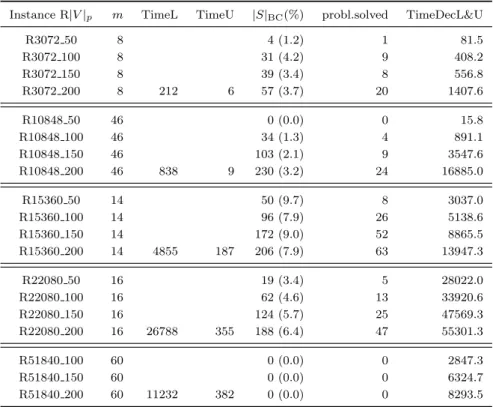
Table 1 shows results obtained from running algorithm DecL&U on instances R|V |p. The
first column identifies the instance (which specifies the number of vertices and the number of facilities to install). The second column indicates the number of components m of the graph. In columns “TimeL” and “TimeU ” we report the CPU time in seconds to obtain initial matrices L and U , respectively, for each graph and for p = 200 (i.e., the largests (p − m + 1) × m matrices for each graph, as for instances where p < 200 the corresponding matrices are submatrices of these). Column “|S|BC” gives the number (and percentage w.r.t. (p − m + 1) × m) of active subproblems
Algorithm DecL&U (Decomposition using matrices L and U) : Given m connected components Gk of a weighted graph G = (V, A, w); number p of facilities to install (at least one
in each component); and optimality gap δ ≥ 0, determines a δ-approximate (optimal if δ = 0) p-median solution on G.
Compute matrices L and U as described in Section 3 S ← {(q, k) : lqk< uqk}
u∗ ← the optimal value of the LSP w.r.t. U Update L, U and S using procedure RAS zL← an optimal LSP solution w.r.t. matrix L
l∗ ←P
k
P
qLqkzLqk
while u∗> (1 + δ) l∗ do
Determine (q, k) such that (UqkzqkL − LqkzqkL) is maximum
Solve subproblem (q, k) (i.e. the q-median problem on graph Gk)
wqk∗ ← the weight of the optimal solution lkl← wqk∗
ukl← w∗qk
S ← S \ {(q, k)}
u∗← the optimal value of the LSP w.r.t. U update L, U and S using procedure RAS zL← an optimal LSP solution w.r.t. matrix L l∗←P
k
P
qLqkzqkL
end while
before the do while cycle of algorithm DecL&U is executed. The number of subproblems that were solved to optimality is given in column “prob.solved”, and column “TimeDecL&U” indicates the CPU time in seconds that DecL&U took to solve the p-median problem (not including the computational time used to obtain matrices L and U ).
Table 1: Results obtained by algorithm DecL&U on real ODMP instances R|V |p. Instance R|V |p m TimeL TimeU |S|BC(%) probl.solved TimeDecL&U
R3072 50 8 4 (1.2) 1 81.5 R3072 100 8 31 (4.2) 9 408.2 R3072 150 8 39 (3.4) 8 556.8 R3072 200 8 212 6 57 (3.7) 20 1407.6 R10848 50 46 0 (0.0) 0 15.8 R10848 100 46 34 (1.3) 4 891.1 R10848 150 46 103 (2.1) 9 3547.6 R10848 200 46 838 9 230 (3.2) 24 16885.0 R15360 50 14 50 (9.7) 8 3037.0 R15360 100 14 96 (7.9) 26 5138.6 R15360 150 14 172 (9.0) 52 8865.5 R15360 200 14 4855 187 206 (7.9) 63 13947.3 R22080 50 16 19 (3.4) 5 28022.0 R22080 100 16 62 (4.6) 13 33920.6 R22080 150 16 124 (5.7) 25 47569.3 R22080 200 16 26788 355 188 (6.4) 47 55301.3 R51840 100 60 0 (0.0) 0 2847.3 R51840 150 60 0 (0.0) 0 6324.7 R51840 200 60 11232 382 0 (0.0) 0 8293.5
The results on Table 1 seem very encouraging on the usefulness of the decomposition algorithm DecL&U to handle large problems. The number of active subproblems before the do while cycle was always below 10%. In four instances the optimal values were obtained by RAS algorithm, with no need to solve to optimality any problem, i.e., the lower and upper bounds derived in Section 3 combined with the elimination procedure described in Section 4 were sufficient to prove optimality. Not surprisingly, it can be found that the number of subproblems solved to optimality, with the exception of instances R3072 100 and R3072 150, increases as p increases. Among the 20 instances, only in 7 the number of subproblems solved was greater than the number of components. In the worst case, instance R15360 200, it was necessary to solve 63 subproblems, which corresponds to 2.4% of the number of subproblems. Overall, the average number of problems that were solved to optimality was less than 1% of the number of subproblems. Regarding the running times, as expected, the time to compute the matrix of lower bounds L largely exceeded the time to obtain the matrix U of upper bounds. Even applying the Fibonacci procedure that significantly reduced the need to obtain the dual optimal values D(q) for each of the 3.120 subproblems on instance R22080 200, it took about 7.5 hours to compute matrix L. Also the time to obtain L for instance R51840 200, slightly exceeded 3 hours. Much more time would be needed if that expedite procedure were not used. In those instances, especially in instance R22080 200, some of the components have many vertices (one of the components in R22080 200 has 6144 vertices). The times to compute U were much smaller (maximum about 6.4 minutes). Total times (not including the time for computing matrices L and U ) vary from 15.8
seconds (R10848 46), where no subproblem was solved, to 15.4 hours (R22080 200). Instances R22080 50, . . . ,R22080 200 were the most time consuming, and this is due to the large number of vertices in some of the 16 components of the graph. Nevertheless, the decomposition algorithm was capable to produce presumably optimal p-median solutions (optimality gap δ = 0.001) for each of these large real instances. (For some of these instances the optimal solutions were not known before.)
We also tested the decomposition algorithm DecL&U on simulated data generated as follows. We considered graphs with |V | = 1000 vertices and number of components m equal to 5 and 10 (0.005|V | and 0.01|V |, respectively). For each m, the number of vertices in each of the m components was determined uniformly selecting a partition rk, k = 1, . . . , m, of |V | = 1000 into
exactly m parts. We generated each component Gkof graph G uniformly selecting in a square rk
points for vertices of Gk, and assigning the cost of each arc connecting vertice i to j the Euclidean
distance between points i and j. We used function rand partitions from package ‘rpartitions’ [11] of R Statistical Software [13] to generate 5 uniform partitions for each m, thus producing a total of 10 different graphs. For each graph with m = 5 components we settled the number of medians p to be equal to 10, 20 and 50 (0.01|V |, 0.02|V | and 0.05|V |), and for each graph with m = 10 components we considered p equal to 20 and 50. We represent these instances by S1000m,p,l, with l = 1, . . . , 5, corresponding to each of the 5 partitions of m.
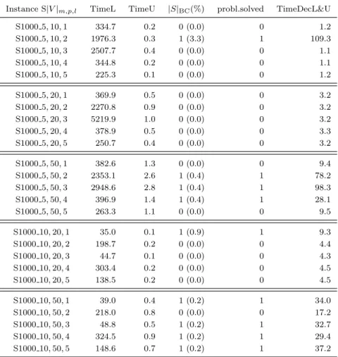
The main results of running algorithm DecL&U on Euclidean simulated instances S1000m,p,l
are given in Table 2 which reads as Table 1. These instances are much easier to solve than the ODMP instances. The number of subproblems solved was either zero (the elimination procedure solved the problem) or one. With respect to running times, the construction of the matrix of lower bounds L was also very time consuming. Specially for instances S10005,p,2 and S10005,p,3
it took quite some time to compute matrix L (more than one hour on instance S10005,p,3). This
is justified by the large number of vertices in one of the components of the graph of each of these instances. Instance S10005,p,2 has a component with 734 vertices, and one of the components of
instance S10005,p,3 includes 779 vertices. For the remaining instances, the times for calculating L
were less than 7 minutes. The largest component of the graphs of all these instances includes 425 vertices. Conversely, the times to compute U were negligible (at most 1.4 seconds). The time of the do while cycle depends on whether there is one subproblem to solve or not, was in all cases less than 3 minutes.
Table 2: Results obtained by algorithm DecL&U on simulated Euclidean instances S|V |m,p,l. Instance S|V |m,p,l TimeL TimeU |S|BC(%) probl.solved TimeDecL&U
S1000 5, 10, 1 334.7 0.2 0 (0.0) 0 1.2 S1000 5, 10, 2 1976.3 0.3 1 (3.3) 1 109.3 S1000 5, 10, 3 2507.7 0.4 0 (0.0) 0 1.1 S1000 5, 10, 4 344.8 0.2 0 (0.0) 0 1.1 S1000 5, 10, 5 225.3 0.1 0 (0.0) 0 1.2 S1000 5, 20, 1 369.9 0.5 0 (0.0) 0 3.2 S1000 5, 20, 2 2270.8 0.9 0 (0.0) 0 3.2 S1000 5, 20, 3 5219.9 1.0 0 (0.0) 0 3.2 S1000 5, 20, 4 378.9 0.5 0 (0.0) 0 3.3 S1000 5, 20, 5 250.7 0.4 0 (0.0) 0 3.2 S1000 5, 50, 1 382.6 1.3 0 (0.0) 0 9.4 S1000 5, 50, 2 2353.1 2.6 1 (0.4) 1 78.2 S1000 5, 50, 3 2948.6 2.8 1 (0.4) 1 98.3 S1000 5, 50, 4 396.9 1.4 1 (0.4) 1 28.1 S1000 5, 50, 5 263.3 1.1 0 (0.0) 0 9.5 S1000 10, 20, 1 35.0 0.1 1 (0.9) 1 9.3 S1000 10, 20, 2 198.7 0.2 0 (0.0) 0 4.4 S1000 10, 20, 3 44.7 0.1 0 (0.0) 0 4.3 S1000 10, 20, 4 303.4 0.2 0 (0.0) 0 4.5 S1000 10, 20, 5 138.5 0.2 0 (0.0) 0 4.5 S1000 10, 50, 1 39.0 0.4 1 (0.2) 1 34.0 S1000 10, 50, 2 218.0 0.8 0 (0.0) 0 17.2 S1000 10, 50, 3 48.8 0.5 1 (0.2) 1 32.7 S1000 10, 50, 4 324.5 0.9 1 (0.2) 1 29.4 S1000 10, 50, 5 148.6 0.7 1 (0.2) 1 37.2
The very good results obtained with the subproblem elimination algorithm RAS before enter-ing the do while cycle of algorithm DecU&U, have a theoretical explanation. When the decrease of marginal costs is monotone (i.e., the impact on the reduction of the cost decreases as the num-ber of facilities increases), which is a common behaviour of the objective function of p-median problems, the following property holds: if a subproblem (q, k) can be eliminated based on the elimination rule ¯`∗qk > u∗ where u∗ was obtained with s facilities in component k, than all the subproblems (q0, k) with q0 ≤ q if q < s, or all the subproblems (q0, k) with q0 > q if q > s, can also be eliminated. This result is formally stated and proved in the Appendix.
This was exactly what we have observed in the computational tests. After applying algorithm RAS, the resulting set of active subproblems (q, k), for each component k, is formed only with consecutive values of q within an interval containing the number of facilities in component k of the p-median optimal solutions.
From the practical point of view, this result provides insight on which are the subproblems whose bounds should be improved first. The result indicates that the (q, k)-subproblems that are not eliminated by algorithm RAS are those where q is in the neighborhood of the optimal p∗k. As a consequence, one should not spend much computational effort in improving bounds and solving (q, k)-subproblems such that q is far from p∗k. As p∗k is not known in advance, we need to estimate it. Initially, this value is estimated by the number of facilities indicated by the greedy solution, and then by the optimal solution to a LSP in subsequent steps. This is the reason for which we opted to initially improve the bounds on a neighborhood (±3) of the number of facilities defined
by the greedy solution, and for solving a subproblem belonging to an optimal solution of the LSP in each iteration of the decomposition algorithm.
Notice that the “curve of the optimal values” as a function of p is “convex”, in most parts of the domain, as depicted in Figure 1. Thus, even if the monotonicity condition of marginal improvements does not hold for some values of p, it is still reasonable to expect that subproblems (q, k) where q is far from p∗k will be promptly eliminated.
7
Conclusion
We propose a decomposition approach to solve the p-median problem on disconnected graphs. The approach decomposes the p-median problem on graph G into a number of subproblems of much lower sizes. As the number of subproblems can be large and solving all of them may be impractical for many instances, the approach starts to compute a lower bound and an upper bound to approximate the optimal value of each subproblem in order to eliminate subproblems from further search. Then for each iteration the approach solves a selected subproblem, updates the bounds, and eliminates subproblems.
We report results on real ODMP instances and on simulated Euclidean instances that show that using efficiently the elimination procedure more than 90% of the subproblems can be elimi-nated by using the initial bounds. Moreover, in general, only few subproblems need to be solved to optimality in order to obtain the optimal solution of the original p-median problem.
To finish we would like to point out that the decomposition algorithm can also be used to generate feasible solutions for general large size p-median problems, not necessarily defined over disconnected graphs. It suffices to add a step where the original set of locations is partitioned by some appropriate clustering algorithm into m subsets, and ignoring the edges linking nodes in different clusters. Then the proposed decomposition approach can be applied to the resulting disconnected graph. This process can be repeated for different partitions. We plan to explore this in future work.
Appendix
Theorem 7.1. Let u∗ be the value of a feasible solution to problem (2.1)-(2.4) with zsk = 1 (s
facilities are installed in component k); p∗k be the number of facilities in component k ∈ K, of an optimal p-median solution of graph G, and let lS(q) be the lower bound on the optimal value
wS∗(q) of the q-subproblem defined for the subgraph of G containing the components in S ⊆ K. (For S = {k}, we use the notation introduced in Section 3 where lqk denotes the lower bound on
the optimal value w∗qk of the (q, k)-subproblem). If ¯
l∗ik> u∗, (7.1)
and the following monotonicity condition on the decrease on the cost function holds wS∗(q − 1) − wS∗(q) ≥ wS∗(q) − w∗S(q + 1), for S ⊆ K,
and q = |S| + 1, . . . , min{p − m + |S|,P
k∈S|Vk|} − 1,
(7.2)
(a) If i > s, then in every optimal solution p∗k< i. (b) If i < s, then in every optimal solution p∗k> i.
Proof. We only prove (a) since the proof of (b) is similar. We show that if (7.1) and (7.2) hold then l∗i+1,k> u∗. By induction it will follow that ¯l∗i+t,k > u∗, for all possible t > 1.
From (7.2), with S = {k} and q = s + 1, . . . , i, we can derive the following inequality. w∗ik− wi+1,k∗ ≤ w ∗ sk − w ∗ ik i − s . (7.3)
Similarly, with S = K \ {k} and q = p − i, . . . , p − s − 1, we get from (7.2)
wK\{k}∗ (p − i − 1) − wK\{k}∗ (p − i) ≥ w ∗ K\{k}(p − i) − w ∗ K\{k}(p − s) i − s . (7.4)
Using (7.1), we have lik+ lK\{k}(p − i) = ¯l∗ik> u∗ ≥ w∗sk+ w∗p−s,K\{k}. Hence it follows it follows
that wsk∗ − lik< lK\{k}(p − i) − wK\{k}∗ (p − s) ⇒ w ∗ sk− w ∗ ik< w ∗ K\{k}(p − i) − w ∗ K\{k}(p − s).
Since i − s > 0, this implies
w∗sk− w∗ ik
i − s <
w∗K\{k}(p − i) − w∗K\{k}(p − s)
i − s . (7.5)
Combining the inequalities (7.3), (7.4), (7.5), we have
wik∗ − w∗i+1,k< wK\{k}∗ (p − i − 1) − w∗K\{k}(p − i),
and finally
wi+1,k∗ + w∗K\{k}(p − i − 1) > wik∗ + wK\{k}∗ (p − i) ≥ lik+ lK\{k}(p − i) = ¯lik∗ > u ∗.
Acknowledgements
This research was partially supported by the Funda¸c˜ao para a Ciˆencia e a Tecnologia (Por-tuguese Foundation for Science and Technology) through projects UID/MAT/04106/2013 (A. Agra and C. Requejo) and UID/MAT/00297/2013 (J.O. Cerdeira).
References
[1] A. Agra, D. Cardoso, J. Cerdeira, M. Miranda, and E. Rocha. Solving huge size instances of the optimal diversity management problem. Journal of Mathematical Sciences, 161:956–960, 2009.
[2] A. Agra, J. Cerdeira, and C. Requejo. Using decomposition to improve greedy solutions of the optimal diversity management problem. International Transactions in Operational Research, 20(5):617–625, 2013.
[3] A. Agra and C. Requejo. The linking set problem: a polynomial special case of the multiple-choice knapsack problem. Journal of Mathematical Sciences, 161:919–929, 2009.
[4] P. Avella, M. Boccia, C. D. Martino, G. Oliviero, A. Sforza, and I. Vasil’ev. A decomposition approach for a very large scale optimal diversity management problem. 4OR, 3:23–37, 2005. [5] O. Briant. ´Etude th´eorique et num´erique du probl`eme de la gestion de la diversit´e. PhD
thesis, Institute Nacional Polytechnique de Grenoble, Grenoble, France, 2000.
[6] O. Briant and D. Naddef. The optimal diversity management problem. Operations Research, 52(4):515–526, 2004.
[7] M. Captivo. Fast primal and dual heuristics for the p-median location problem. European Journal of Operational Research, 52:65–74, 1991.
[8] D. Cardoso and J. Cerdeira. The minimum weight t-composition of an integer. Journal of Mathematical Sciences, 182:210–215, 2012.
[9] M. Daskin and K. Maass. The p-median problem. In G. Laporte, S. Nickel, and F. S. da Gama, editors, Location Science, pages 21–45. Springer International Publishing, 2015. [10] FICO. Xpress Optimization Suite, July 2015.
[11] K. Locey and D. McGlinn. rpartitions: code for integer partitioning. Weecology, Logan, UT, R package version 0.1, 2012.
[12] P. Mirchandani and R. Francis, editors. Discrete Location Theory. John Wiley & Sons, 1990. [13] R Core Team. R: A Language and Environment for Statistical Computing. R Foundation
for Statistical Computing, Vienna, Austria, 2016.
[14] J. Reese. Solution methods for the p-median problem: an annotated bibliography. Networks, 48:125–142, 2006.
[15] C. ReVelle, H. Eiselt, and M. Daskin. A bibliography for some fundamental problem cate-gories in discrete location science. European Journal of Operational Research, 184:817–848, 2008.